Linear system construction of multilateration based on error propagation estimation

R E S E A R C H

Open Access

Linear system construction of

multilateration based on error propagation

estimation

Yanjun Hu

, Lei Zhang

, Li Gao

, Xiaoping Ma

and Enjie Ding

Abstract

Iterative localization algorithms are critical part in the control of mobile autonomous robots because they feed fundamental position information to the robots. In a harsh unknown environment, the estimation of environmental noise is hardly obtained during the movement of the robots. It means that the state-of-the-art methods, which increase localization accuracy using error management, are unsuitable. In this paper, we deduced an upper bound of the localization error without knowing the precise model of environment noise when the anchor nodes have position errors. Utilizing the minimum upper bound, we can construct an optimal localization linear system of iterative localization algorithms based on least square. An algorithm of generating localization linear system is proposed by using the minimum upper bound. The algorithm reduces the impact of the shortage of environmental information on localization error propagation. Our simulation results show that the algorithm is insensitive to noise and can improve the localization accuracy by constructing a proper localization linear system with a high probability.

Keywords:Iterative localization, Error propagation, Upper bound, Orthogonally invariant norms

1 Introduction

Indoor iterative localization algorithm of autonomous robots is an active subject because of the environmental complexity. The coordinates of autonomous robots are the fundamental parameters of robot control [1]. Due to the absence of Global Positioning System signals in an indoor-like environment, the autonomous robots need an iterative localization algorithm to provide their position information. Laser, sonar, infrared, visual sensors, or some combinations of these methods are used to locate the robots [2]. However, those technologies may fail in some harsh environments, such as a firing building which is dusty, smoky, and dark.

Iterative localization based on Received Signal Strength (RSS) is a suitable option to provide the position informa-tion in a harsh scenario [3]. Indoor iterative localizainforma-tion based RSS is exploited in ranging-based techniques, which maps the distance by a measurement of RSS, see

e.g., [4–6]. Since the measurement noise is inevitable in the practical localization system, algorithms are pro-posed to improve the localization accuracy. In those al-gorithms, the key component of decreasing localization error is to estimate the measurement noise. And, those al-gorithms work effectively if the noise is estimated precisely [7]. However, in a harsh scenario, the noise estimation is almost impossible to be achieved because of the insuf-ficiency on measurement noise caused by the robots mobility [8]. A new strategy of improving localization accuracy is needed to solve the problem. Actually, localization accuracy is influenced by the construction of localization linear system (LLS) when least square is used to calculate the position of the unknown node. Therefore, we can decrease localization error by con-structing proper LLS. In this paper, through the study-ing of upper bound of localization error of LLS, an upper bound of error propagation in the localization is proposed. And, an algorithm which can be used to im-prove the localization accuracy without environmental noise estimation, by utilizing the upper bound to gener-ate an optimum LLS.

* Correspondence:[email protected] 2

School of Electrical Engineering and Automation, Jiangsu Normal University, Xuzhou, People’s Republic of China

Full list of author information is available at the end of the article

The paper is organized as following: In Section 2, re-lated works are introduced. In Section 3, the key step of iterative localization is briefly described to introduce the symbols. In Section 4, after introducing the orthogonally invariant norms, it is given that the error upper bound of localization using anchors with localization error. And, an algorithm of improving localization accuracy is proposed by constructing optimum LLS which uses the minimum upper bound. In Section 5, the random and efficient of algorithm are verified by simulations.

2 Related work

The iterative localization algorithm is a distributed, infrastructure-free positioning algorithm to calculate nodes’positions in the ad hoc networks [9, 10], which is a“spreading” process of node information. The process consists of three processes, which are node registry, neighbor selection, and update criterion [11].

The main difference between the iterative localization and the common localization is that the coordinates of located nodes are used or not to calculate the unknown nodes. In iterative localization, there exists unknown nodes that will use the nodes’coordinates which is cal-culated with localization error. It means that anchor node coordinates may or may not have errors in a co-ordinate calculation process. To distinguish the anchor nodes with position error from those nodes with precise coordinates, the anchor nodes without coordinate errors

are named origin-anchors, while the others are called

pseudo-anchors. Based on the notions, a typical iterative localization algorithm carries out in the following steps:

Initiating nodes: Each node in the ad hoc network initiates its coordinate and the coordinate’s errors. Selecting origin-anchors: Three or more nodes are selected as origin-anchors, whose coordinate errors are considered as zero. Then, a relative coordinate system is built by using those nodes.

Generating pseudo-anchors: An unknown node selects at least three located nodes from the neighbor nodes set to calculate its position. After the node is located, this node is updated as a pseudo-anchor.

In this perspective, an iterative localization algorithm is a process of transforming the nodes into the pseudo-anchors. Obviously, the localization accuracy is influenced by the last two steps. The method of selecting origin-anchors is studied, such as choosing the nodes with maximum dens-ity factor [9]. Consider the executing time, the process of pseudo-anchor generation will be executed more fre-quently than the process of origin-anchor selection. Therefore, improving the localization accuracy in the step of generating pseudo-anchors will significantly decrease the localization errors of all pseudo-anchors. To meet the

requirement of improving localization accuracy, physical methods and cyber methods can be used.

In particular, physical methods are based on the idea that the less measurement error is the less localization error is. It improves localization accuracy by using more sensitive sensors. For example, passive broad-band harmonic nonlinear transmission-line tags were used to measure the distance of two nodes [12, 13] or the distance was estimated by using the channel state information [14].

Meanwhile, under the constrains of the measurement accuracy limitation in the physical methods, cyber method is to design algorithms for finding an optimal position estimation of the unknown node. Multilatera-tion based on Least-Squares (MLS) [15] is one widely used cyber method. Also, the localization error of MLS was studied to improve the localization accuracy [16]. Cramer Rao Bound is used to calculate the localization error bound [17–19], in which probability density func-tion of noise is needed to calculate Fisher informafunc-tion matrix. And, localization accuracy was characterized by using a noise covariance bound when anchor nodes have location uncertainty [20]. To calculate localization error accumulating during an iterative process, the mean of localization error was given in the literature [11]. All those literatures assumed that the probability density function or covariance of noise is known. However, ac-cording to the description above, the assumption is not always satisfied in a harsh scenario. The peculiarity of localization in an anonymous environment is noticed [21]. But, the literature is focused on converting the RSS into the distance when little information on the radio propagation model is provided. It is still not studied that how to improve localization accuracy in the scenario of the insufficiency on measurement noise caused by the robots mobility. Xu et al. [22, 23] proposed a crowdsourcing-based framework for processing mobile information and have been proved to be a high accuracy and efficiency.

3 Iterative localization based on least squares

To introduce the notions and symbols used in the follow-ing contents, here, we briefly describe the process of MLS. Let x= (x,y) represents the coordinate of an unknown node located based on an anchor nodes set {xi= (xi,yi)|i= 1,⋯,n} wherenis the cardinality of the anchor nodes set, and ∥ ∥2is the Euclidean norm. Localization based least

squares performs as following:

First, the algorithm collects the measurement data, which is

x−xi

k k2¼d^i ði¼1;⋯;nÞ ð1Þ

whered^idenotes the measurement distance between the

ith anchor node and the unknown node. Squaring both

x

It is obvious that there are n constraints in a

localization system.

Then, ith anchor node is selected as the

benchmark-anchor-node (BAN). Subtracting the ith reference from all other constraints, we have:

2ðxk−xiÞxT¼k kxk 2₂þd^2_k− k kxi 2₂−d^2_i

ð3Þ

wherek≠i;k= 1,⋯,n. After that, we have a localization linear system (LLS) withn−1 equations:

AixT¼bi ð4Þ

The subscriptiofAiandbiemphasizes that theAand

bare generated in the case of choosingith anchor node as BAN.

Finally, using the method of least-squares, the solution

^

x in (4), which is the estimated coordinate of the

un-known node, is obtained

^

x¼ AT_iAi

−1

AT_ibi ð5Þ

The estimation coordinate of pseudo-anchor always deviates its physical coordinate since the measurement error exists. The literatures introduced in Section 2 have studied the methods of improving localization accuracy based on measurement error estimation. Unfortunately, as it is discussed, those algorithms are disabled because of the insufficiency on measurement noise in a harsh scenario. It is noted that the localization is influenced by choosing BAN. Therefore, generating proper LLS is a way to obtain the optimal localization accuracy instead of measurement error estimation.

The following section discusses the upper bound of the localization error propagation. We use the boundary to guide the construction of LLS which can be used in distribution infrastructure-free localization algorithm.

4 Localization error upper boundary of anchors with errors

One character of iterative localization is that the localization error propagates. We deduce an upper bound of the localization error propagation based on orthogon-ally invariant norms. In addition, an algorithm is proposed by using the upper bound as a LLS measurement.

4.1 Orthogonally invariant norms

The orthogonally invariant norms are used to conduct the upper bound of the localization error propagation. The notion and its characters are introduced as follows.

Definition 1 (Orthogonally Invariant Norms (Watson et al., [24]). Consider SVD of a given matrix A, A have singular value decomposition

A¼UΣVT ð6Þ

whereUandVare orthogonal matrices andΣis anm×n

diagonal matrix, where the diagonal terms are the singular values ofAin descending order

σ1≥σ2⋯≥σn ð7Þ

Orthogonally invariant norms can be defined by

A

k k ¼ϕ σð Þ ð8Þ

where σ= (σ1,⋯,σn)Tand ϕ is a symmetric gauge func-tion, such a function satisfies the following conditions:

(1)Φ(x) > 0,x≠0,

Also, the following characters of the norm, which will be used in the Section 4.2, are obtained:

(1)‖AT‖=‖A‖,∀A∈ℂm×n

4.2 Upper boundary of localization error of LLS-RSS iterative algorithm

4.2.1 Upper boundary of localization of error LLS

We propose a lemma which describes the upper bound of localization error for a LLS. The lemma issues an ab-stract but a useful formula for calculating the upper bound of the error propagation.

Theorem 1.Assuming ith anchor node is chosen as the BAN, a LLS is expressed as

^

Ai^xiT¼^bi ð9Þ

where Âi=Ai+ΔÂiis a matrix constructed by anchors’

positions, Airepresents precise physical position of

an-chor nodes, ΔÂiis the coordinate errors of the anchors;

^

bi¼biþΔb^i is a vector collection of the anchors’

pos-ition and the measurement data,bidenotes the noiseless

measurement data, Δb^i represents the noise of the

^

where†i is Moore-Penrose pseudo-inverse of matrixÂi. Then, applying norm characters on (12), an inequality is obtained

^

xiT _{⩽ A}^†

i ₂k kbi 2þ A^†i ₂ Δbi^ ₂ ð13Þ

The inequality can be transformed into

^

are concluded. Using those inequalities, (14) becomes

^

4.2.2 Error upper boundary of LLS-RSS

The Theorem 1 gives a universal upper bound of the meas-urement error. Since RSS is widely used as the measure-ment data, we propose a concrete numeral upper bound of the measurement error of a LLS-based RSS (LLS-RSS). The upper bound will be fundamental of algorithm which can construct the optimum LLS in the next subsection.

To calculate the upper bound of Lemma 1, we need to calculatek, α, andβ. Thekand αare calculable, because all components are only related with known coordinate of anchors (origin-anchors, pseudo-anchors, or combination of them). However, the measurement data noiseΔ^biis

ran-dom and unmeasurable. It makes instantaneous value ofβ

that cannot be calculated. The value can be obtained is the

mean of βwhich is upper boundary. As an extension of

Theorem 1, the mean of error upper bound of LLS-RSS is given by Lemma 2.

Theorem2.In a LLS-RSS expressed asA^ix^iT¼b^iþΔ

^

bi, ΔÂiis a matrix constructed by the minimum upper

bound of localization error of corresponding anchors. If the radio propagation model between ith node and kth node satisfies the model of distance-dependent path loss with log-normal fading, whose parameters areηand Xσi,

and random variable Xσiði¼1;⋯;n−1Þ are independent

and identically distributed, there is

E k k^xi

Proof. According to the radio propagation model of distance-dependent path loss with lognormal fading [25], we have:

Prð Þ ¼dr P0−η10 log10 di

d0 þ

Xσi ð22Þ

The distance between ith anchor and the unknown

node, denoted asdi, should be calculated as

dk¼d010

P0−Pr drð ÞþXσi

However, sinceXσi is a physically immeasurable random

variable, the kth estimated distance, denoted as d^k is calculated as

^

dk¼d010

P₀−Pr drð Þ

10η ð₂₄Þ

Introduce aΔd2, which is defined as

Δd^2_k≜d^2_k−d2_k¼d^2_k 1−10

In a practical localization system, the noise always ex-ists in measurement data. It is defined as

bi_k≜^bi_k− Δb^i_k;1þΔb^i_k;2

dom variables are independent and identically distributed. Use Theorem 1, Combine (25), (29) and norm defin-ition, the (20) and (21) are obtained.

4.3 Optimum algorithm of constructing LLS

Theorem 2 gives the numerical result of localization ac-curacy influenced by node information and measure-ment data. The theorem can handle the situation that the positions of the anchor nodes can exist error. Al-though the error upper bound is calculated in statistical significance, Δbi/bi appears with a high probability,

which is tested in experiments.

Therefore, the minimum upper bound can be used as a localization quality indicator of the LLS. An LLS con-struction algorithm, optimum algorithm of constructing LLS (OAC-LLS) shown as Algorithm 1, is proposed. This algorithm utilizes the minimum upper bound to choose the best candidate from the LLS set with a high probability.

Remark: The environment parameterσ/ηis needed to

calculate the Ei in (19). But, a estimated value can be used. It will not significantly affect the result. It means that the algorithm could be fully“blind”based on an as-sumption value. Of course, any knowledge of parameter can improve the algorithm performance. This conclusion is discussed in Section 5.2.

5 Simulation and discussion

The following assumptions are used in experiments.

(i) We use three origin-anchor nodes, whose coordinates are (0, 0), (50, 0), and (25, 50), respectively. The nodes are numbered by their orders. The fourth node is a pseudo-anchor whose coordinate is (25, 25). The fifth node is a pseudo-anchor.

(ii)The radio propagation model uses distance-dependent path loss with log-normal fading with Gaussian noise N (0,1.5).

(iii) The position of the unknown node is calculated as ^

xm¼ A^T_mA^m

−1_^

AT_mbm.

To distinguish the different LLS, which use different anchor set of origin-anchors or pseudo-anchors, we

add a superscript on Âi to declare the used anchor

nodes. Therefore,A^1₁‐2‐3means the LLS uses three nodes whose numbers are 1, 2, and 3, and 1-st node are chosen as BAN.

5.1 Evaluation indicator

bound. Therefore, the coordinate error is unsuitable to evaluate the algorithm performance.

To evaluate the efficiency of improving accuracy using minimum rough upper bound, we introduce two counters: (a)strict-match-counter(SMC) and (b)slack-match-count

(LMC). The counters work as following:

SMC: Let initial value of SMC be 0. SMC increases 1, if and only if, the minimum of rough upper bound and the minimum of localization absolute error are both obtained whenith anchor is selected as a BAN.

LMC: It is similar to SMC. However, LMC increases 1 when localization absolute error is smallest or

second smallest in the case of the upper bound is minimum with the same BAN.

5.2 Feasibility of the algorithm

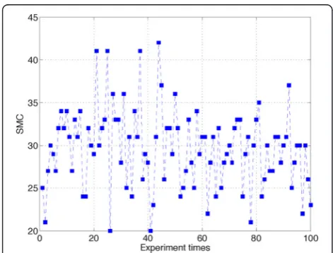
Each value is the match count per 100 times simulations using SMC. The calculation of minimum upper bound usesσ/η= 0.65 in each time.

To calculate the upper bound by using Theorem 2,σ/ηis needed to obtainc. Experiments are implemented to illus-trate the probability of construction optimum LLS varies with σ/η. The fifth node is placed at (25, 6).σ/η= 0.65 is used in each time of calculation of minimum upper bound. As shown in Fig. 1, the probability of construction

optimum LLS varies with σ/η. The curve shows a

Fig. 1Experiments result of probability of construction optimum

LLS varies withσ/η

Fig. 2Experiments result that the minimum upper bound

matches with optimum LLS. The simulation is done 100 × 100 times, and each value is the match count per 100 times simulations using SMC

Fig. 3Experiments result that the minimum upper bound

matches with optimum LLS. The simulation is done 100 × 100 times, and each value is the match count per 100 times simulations using LMC

Fig. 4Each colored block represents the matching counts per 100

trend that the probability is descent while the σ/η is away from the precise value. It means that the

algo-rithm could be fully “blind” on the environment.

Meanwhile, any information of environment, such as

the possible range of σ/η, can greatly improve the

al-gorithm performance.

5.3 Randomness of the algorithm

Experiments are executed to test the randomness of the algorithm. The fifth node is placed at (25, 6), and the ex-periments are executed for 100 × 100 times.

As shown in Fig. 2, if the SMC is selected as an evalu-ation indicator, the mean and standard devievalu-ation of

Fig. 5Localization accuracies vary with different BANs. The unknown node is fixed at (25, 45), and noise is random in each time

probability of choosing best LLS are 0.2959 and 4.57, re-spectively. In the same way, shown in Fig. 3, if LMC is used as an evaluation indicator, the mean and standard deviation of probability of constructing best LLS are 0.3934 and 4.86, respectively. It is noted that there are totally eight LLS can be constructed. The probability choosing optimum LLS is 0.125. Our algorithm can gen-erate the best LLS with a higher probability.

5.4 Effectiveness of the algorithm

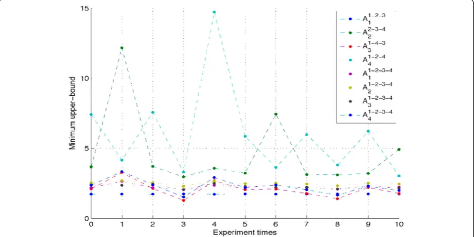
Figure 4 shows the algorithm effectiveness varies with change of the pseudo-anchor’s position. The algorithm is more effective when the fifth node in the triangle zone bordered by the first, third, and fourth nodes. While the fifth node moves away the zone, the probability of con-structing optimum LLS deceases. This phenomenon is reasonable. The localization accuracy of fourth node is stable and precise since the qualities of measurement

data are almost the same (Yang et al., [26]). It means that the fifth node has an additional pseudo-anchor with high accuracy besides four origin-anchors, which make the upper boundary more valuable.

Although the algorithm does not have a good numer-ical performance when the SMC is used as indicator, it is noted that the worst accuracy will not be obtained, as shown in Figs. 5 and 6. In fact, the localization accur-acies are tightly close when the minimum upper bounds are approximately the same, which is shown as enlarged party of Figs. 5 and 6. Therefore, the algorithm is still ef-fective in the perspective of improving localization accuracy.

Additionally, Figs. 5 and 6 show that the curve of absolute errors gently changes when the LLS is the one with minimum upper boundary. It means that the algorithm is stable. The factor of upper bound,

κ=‖Âm‖2‖Âm‖2, is a condition number, which means

that the condition number of LLS will be smaller when the upper bound is minimum. Therefore, the algorithm, which uses minimum upper bound, is in-sensitive to noise.

5.5 Performance evaluation

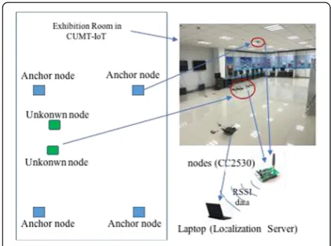
Experiments are done in our exhibition room. The sce-nario is showed as in Fig. 7. All nodes are based on CC2530. Four of them, which are considered as anchor nodes, are fixed on the ceiling. The others are consid-ered as unknown nodes. A laptop is used to sample data and servers as localization server.

Figure 8 illustrates the cumulative distribution func-tion (CDF) of localizafunc-tion errors. The experiment results show that the error falls within the range of 2 m for over 90 % of points, and the 50 % accuracy is less than 1.2 m. The algorithm 1 has a better performance than the

Fig. 7Exhibition room

algorithm which BAN is chosen random. The probability choosing optimum LLS is 0.125 since there are totally eight LLS that can be constructed. However, this prob-ability can approach 0.45 as simulated in Section 5.3. Therefore, we can obtain more accurate coordinate compared to the coordinate obtained when BAN is ran-dom selected.

5.6 Computational complex

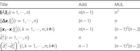
In some application of mobile autonomous robots, the energy consumption and computation ability are con-strained. It requires the localization to be realized on-chip. Computational complexity, which is defined as the number of operations performed by the algorithm [27], is always used to evaluate the possibility implemented on chip.

Algorithm 1 consists of a choosing BAN process and a least-squares algorithm. Assume the algorithm is used in 2D localization, in which casexi,Δxi(i= 1,⋯,n) are two dimensional vectors. The time complexity of least-squares algorithm will be O(n3). To find the best BAN, we first executenloops to obtainEi(i= 1,⋯,n), then we

find the minimumEmwhich is the best BAN. It is noted

that A^†_{i 2}, ‖Âi‖2, kΔxkk22, kxk−xik22, d^k2, and d^2i−d^2k

2

are repeated used in algorithm. The time complexity of

^

A†_i is 64n+ 96 +O(2n) when using Matlab pinv func-tion. The cost functions of other terms are shown as Table 1.

Therefore, the time complexity of algorithm 1 isO(3n3). The algorithm is more complex than the least-squares al-gorithm. It is reasonable because the algorithm trades computational complex off for localization accuracy. It is also noticed thatnis the anchor node number, which is a small value in practice.

6 Conclusions

An upper bound of error propagation of iterative localization is derived, which can be used in the situation that the precise distribution of the environment noise is unknown. The minimum upper bound is adopted to evaluate the localization result of LLS with certain meas-urement data. With this method, an optimum algorithm of constructing LLS is proposed. Even when the environ-ment noise is unknown or unpriced evaluated, the

algorithm still can construct the proper LLS with highly probability, which means it can still obtain the best localization accuracy with high probability.

Acknowledgements

This work is supported partly by the National Key Technology Research and Development Program of the Ministry of Science and Technology of China under grant (no: 2013BAK06B05) and the National Natural Science Foundation of China under grant (no: 61303183).

Competing interests

The author declares that he has no competing interests.

Author details

1_{IoT Perception Mine Research Center, China University of Mining and}

Technology, Xuzhou, People’s Republic of China.2School of Electrical Engineering and Automation, Jiangsu Normal University, Xuzhou, People’s Republic of China.3_{School of Information and Electrical Engineering, China} University of Mining and Technology, Xuzhou, People’s Republic of China.

Received: 13 March 2016 Accepted: 14 June 2016

References

1. J Fink, A Ribeiro, V Kumar, Robust control for mobility and wireless communication in cyber-physical systems with application to robot teams. Proc IEEE100(1), 164–178 (2012)

2. L Ojeda, D Cruz, G Reina, J Borenstein, Current-based slippage detection and odometry correction for mobile robots and planetary rovers. Robotics, IEEE Transactions on22(2), 366_–378 (2006)

3. SS Saad, ZS Nakad, A standalone RFID indoor positioning system using passive tags. IEEE Trans Ind Electron58(5), 1961–1970 (2011)

4. X Li, Collaborative localization with received signal strength in wireless sensor networks. Vehicular Technology, IEEE Transactions on56(6), 3807_–3817 (2007) 5. Z Ma, W Chen, KB Letaief, Z Cao, A semi range-based iterative localization

algorithm for cognitive radio networks. Vehicular Technology, IEEE Transactions on59(2), 704–717 (2010)

6. G Wang, K Yang, A new approach to sensor node localization using RSS measurements in wireless sensor networks. Wireless Communications, IEEE Transactions on10(5), 1389–1395 (2011)

7. MR Gholami, EG Ström, H Wymeersch, Upper bounds on position error of a single location estimate in wireless sensor networks. Eurasip Journal on Advances in Signal Processing1, 1–14 (2014)

8. P Dhakal, D Riviello, F Penna, Impact of noise estimation on energy detection and eigenvalue based spectrum sensing algorithms. IEEE International Conference on Communications IEEE, 1367_–1372 (2014) 9. SČapkun, M Hamdi, JP Hubaux, Gps-free positioning in mobile ad hoc

networks. Clust Comput5(2), 157–167 (2002)

10. LJ Zamorano, L Nolte, AM Kadi, Z Jiang, Interactive intraoperative localization using an infrared-based system. Neurol Res15(5), 290_–298 (1993) 11. J Liu, Y Zhang, F Zhao, Robust distributed node localization with error

management, inProceedings of the 7th ACM international symposium on Mobile ad hoc networking and computing, 2006, pp. 250–261

12. E DiGiampaolo, F Martinelli, Mobile robot localization using the phase of passive UHF RFID signals. IEEE Trans Ind Electron61(1), 365–376 (2014) 13. Y Ma, EC Kan, Accurate indoor ranging by broadband harmonic generation

in passive NLTL backscatter tags. Microwave Theory and Techniques, IEEE Transactions on62(5), 1249_–1261 (2014)

14. Z Yang, Z Zhou, Y Liu, From RSSI to CSI: indoor localization via channel response. ACM Computing Surveys (CSUR)46(2), 25 (2013)

15. A Savvides, H Park, MB Srivastava, The bits and flops of the n-hop multilateration primitive for node localization problems, inProceedings of the 1st ACM international workshop on Wireless sensor networks and applications, 2002, pp. 112–121

16. IA Mantilla-Gaviria, M Leonardi, G Galati, Localization algorithms for multilateration (MLAT) systems in airport surface surveillance. Signal Image & Video Processing9(7), 1–10 (2014)

17. C Chang, A Sahai, Cramer-rao-type bounds for localization. EURASIP Journal on Applied Signal Processing2006, 1–13 (2006)

18. EG Larsson, Cramer-Rao bound analysis of distributed positioning in sensor networks. Signal Processing Letters, IEEE11(3), 334–337 (2004)

19. RL Moses, D Krishnamurthy, RM Patterson, A self-localization method for wireless sensor networks. EURASIP Journal on Applied Signal Processing

2003(4), 348–358 (2003)

20. A Savvides, WL Garber, RL Moses, MB Srivastava, An analysis of error inducing parameters in multihop sensor node localization. Mobile Computing, IEEE Transactions on4(6), 567_–577 (2005)

21. J Koo, H Cha, Localizing WiFi access points using signal strength. Communications Letters, IEEE15(2), 187–189 (2011)

22. Z. Xu et al. Crowdsourcing based description of urban emergency events using social media big data. IEEE Transactions on Cloud Computing,10. 1109/TCC.2016.2517638.

23. Z. Xu et al. Crowdsourcing based social media data analysis of urban emergency events. Multimedia Tools and Applications, 10.1007/s11042-015-2731-1. 24. GA Watson, Characterization of the subdifferential of some matrix norms.

Linear Algebra Appl170, 33–45 (1992)

25. M Shin, I Joe, An indoor localization system considering channel interference and the reliability of the RSSI measurement to enhance location accuracy. International Conference on Advanced Communication Technology IEEE, (2015)

26. Z Yang, Y Liu, Quality of trilateration: Confidence-based iterative localization. Parallel and Distributed Systems, IEEE Transactions on21(5), 631–640 (2010) 27. M Sipser,Introduction to the Theory of Computation, vol. 2 (Thomson Course

Technology, Boston, 2006)

Submit your manuscript to a

journal and benefi t from:

7 Convenient online submission

7 Rigorous peer review

7 Immediate publication on acceptance

7 Open access: articles freely available online

7 High visibility within the fi eld

7 Retaining the copyright to your article