R E S E A R C H
Open Access
Fourth-order compact finite difference
method for solving two-dimensional
convection–diffusion equation
Lingyu Li
1, Ziwen Jiang
1*and Zhe Yin
1*Correspondence: [email protected] 1College of Mathematics and
Statistics, Shandong Normal University, Jinan, China
Abstract
A fourth-order compact finite difference scheme of the two-dimensional
convection–diffusion equation is proposed to solve groundwater pollution problems. A suitable scheme is constructed to simulate the law of movement of pollutants in the medium, which is spatially fourth-order accurate and temporally second-order accurate. The matrix form and solving methods for the linear system of equations are discussed. The theoretical analysis of unconditionally stable character of the scheme is verified by the Fourier amplification factor method. Numerical experiments are given to demonstrate the efficiency and accuracy of the scheme proposed, and these show excellent agreement with the exact solution.
MSC: 65N06; 65N15; 65N22
Keywords: Convection–diffusion equation; Compact finite difference method;
Fourth-order accuracy; Numerical experiments
1 Introduction
In recent years, more and more attention has been paid to the movement of pollutants in groundwater by mathematical modeling [1]. The prediction and evaluation of ground-water dynamic movement and solute transport are important tasks for agricultural pol-lution and groundwater development [2]. A large number of mathematical models and a variety of effective numerical methods have been widely used to simulate the movement of contaminated groundwater. Convection–diffusion equation is a class of very important equations, it can describe many physical phenomena, such as atmospheric pollutants, dis-tribution and diffusion of the oceans and rivers, heat conduction and so many other phys-ical problems even including bacterial concentration. However, from the existing research results, we could only get the analytical solutions of a few classic models. In the process of dealing with practical problems, for many mathematical models, especially partial differ-ential equations, their analytical solutions are not available in general. Therefore, research for the numerical solutions of partial differential equations is very necessary [3].
During the last three decades, the numerical solution of the convection–diffusion equa-tion has been developed by all kinds of methods, for example, the finite difference method [4], the finite element method [5, 6], the finite volume method [7], the spectral ele-ment method [8] and even the Monte Carlo method [9]. But the characteristics of the
two-dimensional convection–diffusion equation and the complexity of the mathematical model are a challenge to numerical computation, so constructing the simple and efficient numerical scheme needs to be further studied. A finite difference method is one of the effective and flexible methods to solve the numerical solution of partial differential equa-tions with initial boundary value [10].
For the traditional finite difference methods, a classical spatial discretization, such as the second-order central difference scheme, fails to approach the exact solution of most equations; for obtaining a more accurate numerical solution one needs to add more nodes and use smaller mesh sizes, which would require more storage space and computing time [11]. In order to get more accurate results for constant mesh size, we have to increase the order of accuracy of the numerical approximation, which, in turn, means enlarging the stencil of grid points [12]. However, this results in some problems, for instance, the difficult treatments of the boundary conditions, the approximation of the points next to the boundaries, and the increasing of the bandwidth of the stiffness matrix. For many application problems, it is desirable to use higher-order numerical methods to obtain an accurate solution.
In terms of the above reasons, a compact finite difference scheme is desired to solve lots of differential equations numerically [13–16]. One can compute more accurate solutions using limited grid sizes through developing high-order compact finite difference schemes. Significant work in this field has been done by Turkel and Singer [17] in 1998. In recent years, the high accuracy compact difference method has attracted more and more atten-tion; see [18–22]. Using a Taylor series expansion, Sari et al. [14] developed a tenth-order finite difference scheme, proposed to solve one-dimensional advection–diffusion equa-tion. Gurarslan et al. [16] presented a sixth-order compact difference scheme in space and a fourth-order Runge–Kutta scheme in time to produce numerical solutions of the one-dimensional advection–diffusion equation, it has been seen to be very accurate in solving the contaminant transport equation forPe≤5. Based on the Grünwald–Letnikov discretization of the Riemann–Liouville derivative, Cui obtained a fully discrete implicit scheme after approximating the second-order derivative with respect to space by the compact finite difference [19]. Li presented an efficient and stable compact fourth-order method for the phase field crystal equation [21]. Kaysar et al. gave an useful and efficient compact finite difference approximation of a fourth-order scheme for solving linear one-dimensional convection–diffusion equation [22]. All in all, there is a renewed interest in the development and application of compact finite difference methods for the numerical solution of the convection–diffusion equations.
in a porous medium. At every stage, contaminant is injected at any region point and at arbitrary time in the river. Applying the mathematical software MATLAB, a numerical simulation is carried out on the problem of water pollution–diffusion to verify the validity and practicability of the model and algorithm. Numerical examples are given to illustrate the accuracy and reliability of the proposed scheme, so as to provide an important basis for water pollution accident disaster emergency disposal and decision-making for envi-ronmental protection personnel dealing with a water pollution incident, to be used as a reference.
The paper is organized as follows: in Sect.2, we present a fourth-order compact dif-ference scheme, in which the Crank–Nicolson scheme is used for temporal discretiza-tion and a fourth-order compact finite difference scheme dealing with a one-dimensional convection–diffusion equation is applied to the spatial discretization. In Sect.3, the ma-trix form for the difference scheme is given, and the solving methods for the linear system of equations are discussed. In Sect.4, the theoretical analysis, the Fourier method, namely the amplification factor method (or von Neumann condition) of the proposed scheme is presented. Finally, numerical examples are provided in Sect.5, the numerical results shown in tables and figures derive the accuracy and prove the convergence order of the scheme, they are in agreement with our theoretical analysis. The paper concludes with a summary in Sect.6.
2 Fourth-order compact finite difference scheme
In this paper, we consider the following two-dimensional convection–diffusion equation, which is used widely to simulate the motion process of the contaminant in groundwater flow and the water flow with any chemical solute. Here we take the seepage area as an infinite plane, assume the groundwater flow belongs to the one-dimensional cases, the diffusion of pollutants is a two-dimensional dispersion in a porous medium, and the con-taminantf(x,y,t) is injected at any region point (x,y) and at any timetin the river.
Let⊂R2with boundary. We write ⎧
⎪ ⎪ ⎨ ⎪ ⎪ ⎩
∂C
∂t =Dx
∂2C
∂x2 +Dy∂ 2C
∂y2 –v∂∂Cx +f, (x,y)∈,t> 0,
C(x,y, 0) =C0(x,y), (x,y)∈,
C(x,y,t) =g(x,y,t), (x,y)∈,t> 0,
(1)
The analytical solution for Eqs. (1) is not available easily, the purpose of this paper is to improve the accuracy in spatial direction, we suggest a fourth-order compact difference scheme. In order to present our scheme, we first introduce some essential notations, which will be used later.
Discretizing the spatial region firstly, let N andM be two positive integers, so that the step sizes are hx= LNx,hy=
Ly
M, under this condition, the spatial nodes can be de-noted by (xi,yj), namely,xi=ihx,i= 0, 1, . . . ,N– 1,N;yj=jhy,j= 0, 1, . . . ,M– 1,M. Let
¯
h={(xi,yj)|0≤i≤N, 0≤j≤M},h=¯h∩,h=¯h∩. For simplicity, introduce
ω={(i,j)|(xi,yj)∈h},σ={(i,j)|(xi,yj)∈h}, then we haveω¯=ω∪σ. DefineUh={u|u= {uij|(i,j)∈ ¯ω}}, for anyu∈Uh, similar to Ref. [24], introducing the following notations of difference quotients:
xuij=
ui+1,j–ui–1,j 2hx
, δ2xuij=
ui–1,j– 2uij+ui+1,j h2
x
, δ2yuij=
ui,j–1– 2uij+ui,j+1
h2 y
.
Next, for the temporal approximation, take a positive integerK, partition the interval [0,T] intoKequal parts of widthτ=TK; we have the following notations:
tn=nτ, τ ={tn|0≤n≤K}, tn+12 =
tn+tn+1
2 , n= 0, 1, . . . ,K– 1,
whereτ is called the temporal step size.
SetUτ ={w|w= (w0,w1, . . . ,wK)T}, for anyw∈Uτ, introducing some notations as
fol-lows:
wn+12 =1 2
wn+1+wn, δtwn+ 1 2 =1
τ
wn+1–wn, n= 0, 1, . . . ,K– 1.
Define grid functions on¯h×τ,Cijn=C(xi,yj,tn), (i,j)∈ ¯ω, 0≤n≤K. Following Refs. [25,26], the two-dimensional convection–diffusion equation in Eqs. (1) can be rewritten as the following two equations:
Dx
∂2C
∂x2 +v
∂C
∂x =f–
∂C
∂t –Dy
∂2C
∂y2 , (x,y)∈,t> 0, (2)
–Dy
∂2C
∂y2 =f–
∂C
∂t –Dx
∂2C
∂x2 +v
∂C
∂x , (x,y)∈,t> 0. (3)
Next, we only need to consider the compact difference scheme with Eq. (2) and Eq. (3), respectively.
For Eq. (2), considering it at the point (xi,yj,tn+12), we have
Dx
∂2C
∂x2(xi,yj,tn+12) +v
∂C
∂x(xi,yj,tn+12) =f(xi,yj,tn+12) – [
∂C
∂t(xi,yj,tn+12) –Dy
∂2C
∂x2(xi,yj,tn+12),
Consider the one-dimensional steady convection–diffusion equation [24]
–α∂
2u
∂x2 +β
∂u
∂x =f(x), (5)
whereαis the constant conductivity,βis a constant representing the convective velocity, f is a sufficiently smooth function ofx, andumay represent the concentration of a solute,
vorticity, heat, etc.
Its three point fourth-order compact scheme is as follows:
–
α+β 2h2
12α δ
2
xu(xi) +βxu(xi) =
1 +h 2
12
δ2x–β
αx f(xi), (6)
where
xu(xi) =
u(xi+1) –u(xi–1) 2h
and
δ2xu(xi) =
u(xi+1) – 2u(xi) +u(xi–1)
h2
are the central difference approximations for the first and second derivatives. We think of the right term
f(xi,yj,tn+12) – [
∂C
∂t(xi,yj,tn+12) –Dy
∂2C
∂x2(xi,yj,tn+12)
of Eq. (4) as a whole, similar to the right termf of Eq. (5), using the method of Eq. (6), taking the Taylor formula into account [27], applying the Taylor expansion for Eq. (4); it generates
–
Dx+ v2h2
x 12Dx
δx2Cn+
1 2
ij +vxC n+12 ij
=
1 +h 2 x 12
δ2x– v
Dx
x f n+12 ij –
∂C
∂t –Dyδ
2 yC |
n+12 ij
+Rn+
1 2 1ij ,
(i,j)∈ω, 0≤n≤K– 1, (7)
where the truncation error is
Rn+
1 2 1ij =O
h4x, (i,j)∈ω, 0≤n≤K– 1. (8)
Considering Eq. (3) at the point (xi,yj,tn+1
2), we have
–Dy
∂2C
∂y2(xi,yj,tn+12) =f(xi,yj,tn+12) –
∂C
∂t(xi,yj,tn+12) –Dx
∂2C
∂x2(xi,yj,tn+12) +v
∂C
∂x(xi,yj,tn+12)
(i,j)∈ω, 0≤n≤K– 1. (9)
For the interior nodes of the spatial of Eq. (3), we use the derivative type fourth-order compact differential formula to deal with the one-dimensional convection–diffusion equation [22].
For convenience, we define a compact difference operator byB[12], for anyu∈Uh,
(Bu)ij= ⎧ ⎨ ⎩
ui,j–1+10uij+ui,j+1
12 , 1≤i≤N, 1≤j≤M– 1,
uij, 1≤i≤N,j= 0,M.
(10)
By Lemma 1.2(g) [12]: Ifg(x)∈C6[c–h,c+h], then we have
1 12
g(c–h) + 10g(c) +g(c+h)= 1
h2
g(c–h) + 10g(c) +g(c+h)+ h 4
240g 6(ξ6),
whereξ6∈(c–h,c+h),h> 0 andcare two positive constants. We have
B∂2u
∂y2(xi,yj,tn) =δ 2 yunij+
h4y
240
∂6u
∂y6(xi,ξjk,tn), (11) where 1≤i≤N, 1≤j≤M– 1, 1≤n≤K, andξjk∈(yj–1,yj).
Apply compact difference operatorBto both sides of Eq. (9), combine with Eq. (11); we have
–Dyδy2C n+12 ij
= 1 12
f(xi,yj,tn+12) –
∂C
∂t(xi,yj,tn+12) –Dx
∂2C
∂x2(xi,yj,tn+12) +v
∂C
∂x(xi,yj,tn+12) + 10
f(xi,yj,tn+12) –
∂C
∂t(xi,yj,tn+12) –Dx
∂2C
∂x2(xi,yj,tn+12) +v
∂C
∂x(xi,yj,tn+12) +
f(xi,yj,tn+12) –
∂C
∂t(xi,yj,tn+12) –Dx
∂2C
∂x2(xi,yj,tn+12) +v
∂C
∂x(xi,yj,tn+12) + h
4 y 240
∂6u
∂y6(xi,ξjk,tn), (i,j)∈ω, 0≤n≤K– 1. (12) It is easy to observe that Eq. (12) is equal to the following form:
–Dyδy2C(xi,yj,tn+12)
=
1 +h 2 y 12δ
2 y
f(xi,yj,tn+12) –
∂C
∂t(xi,yj,tn+12) –Dx
∂2C
∂x2(xi,yj,tn+12) +v
∂C
∂x(xi,yj,tn+12)
+ h 4 y 240
∂6u
∂y6(xi,ξjk,tn),
Taking the Taylor formula into account again, applying the Taylor expansion for Eq. (13),
where the truncation error is
Rn+
For the time term of Eq. (16), we make a Crank–Nicolson (C-N) time discretization, notic-ing the former notations, we can construct
Taking the initial and boundary conditions of Eq. (1) into account, we have
Cij0= 0, (i,j)∈ω,
Cijn=g(xi,yj,tn), (i,j)∈σ, 0≤n≤K.
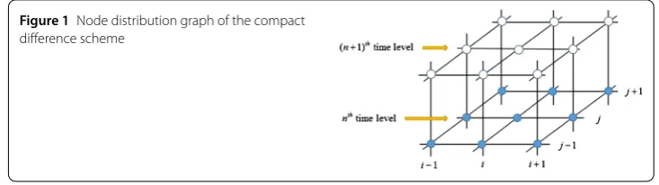
Figure 1Node distribution graph of the compact difference scheme
Ignoring the higher-order termsRn+
1 2
ij in (17), and replacingCnijwith its approximation cn
ij, the compact difference scheme of Eq. (1) can be obtained,
⎧
Theorem 2.1 The truncation error of the compact finite difference scheme(19)is
Rnij=Oτ2+h4x+hy4, (i,j)∈ω, 0≤n≤K. (20)
3 Matrix form of the numerical scheme
The numerical scheme of the convection–diffusion equation plays a very important role in computational fluid dynamics to simulate flow problems [20]. Therefore, accurate and stable difference schemes are of vital importance. To achieve the unconditional stability, we resort to the Crank–Nicolson method for a time discretization of Eq. (19). Notice the notations defined in Sect.2for the difference scheme (19), which will result in a system of algebraic equations that is sparse; the existence and uniqueness of the solution of the scheme (19) are easily known by the positive definite property. We have
–1
p7=
We can give the matrix form of the scheme by
E3=
By simply calculating, we can see that the matrix P2is the same as the matrix P3 abso-lutely. So, we can further write (24) as
The coefficient matrix of the above linear equations is a three diagonal block matrix, and each row has at most nine nonzero elements, therefore we can rewrite the scheme (24) in the following matrix form:
E= ⎛ ⎜ ⎜ ⎜ ⎜ ⎜ ⎜ ⎜ ⎝
E1 E2
E3 E1 E2 . .. ... ...
E3 E1 E2
E3 E1 ⎞ ⎟ ⎟ ⎟ ⎟ ⎟ ⎟ ⎟ ⎠ .
Those three matrices are all strictly diagonally dominant tridiagonal matrices, which guarantees the existence and uniqueness of the solution.
4 Stability analysis
For the presentation of the theoretical analysis, we makef = 0 of the first equation in Eqs. (1) for convenience [1]. Assuming that the boundary conditions are accurate, we ap-ply the Fourier method to the relative difference equation, by calculating the amplification factor to obtain an algebraic criterion for the stability analysis of the scheme (19). With-out loss of generality, we chooseDx,Dyandvas constants. Following the von Neumann condition [28] for linear stability, we assume that the numerical solution can be expressed in the form of a Fourier series [20].
Let
cnij=ηne √
–1(iξxhx+jξyhy), (26)
where ηnis the amplitude at time leveln,√–1 is called the imaginary unit,ξx andξy represent the wave numbers in thexandydirections, respectively, theξxhxandξyhyare named phase angles.
The amplification factor is defined by
G(ξx,ξy,τ) =
ηn+1
ηn . (27)
Substituting the expression ofcnij+1andcnijinto Eq. (25), combining Eq. (26) with Eq. (27), the amplification factor can be written as
G(ξx,ξy,τ) = n
m, (28)
where
n=(q1+ 2q4) + (q2+q3)γ1– 4q4γ3+ (q6+q7)(γ4+γ6)
+i(q2–q3)γ2+ (q6–q7)(γ5+γ7)
,
m=(p1+ 2p4) + (p2+p3)γ1– 4p4γ3– (p6+p7)(γ4+γ6)
+i(p2–p3)γ2– (q6–q7)(γ5+γ7)
,
and
γ1=cosξxhx, γ2=sinξxhx, γ3=sin2
ξyhy
2 , γ4=cos(ξxhx+ξyhy),
γ5=sin(ξxhx+ξyhy), γ6=cos(ξxhx–ξyhy), γ7=sin(ξxhx–ξyhy).
For stability, it has to satisfy the following condition [28]:
G(ξx,ξy,τ)≤1. (30)
Referring to the method of Ref. [29], let
G(ξx,ξy,τ)2= p
q. (31)
We just need to compare the relationship betweenpandq. It is sufficient thatp–q≤0, that is to say, then Eq. (30) is proved.
Imposing that condition directly on Eq. (28), it yields
p–q= (q1+ 2q4+p1+ 2p4)(q1+ 2q4–p1– 2p4)
+ (q2+q3+p2+p3)(q2+q3–p2–p3)γ12+ 16(q4+p4)(q4–p4)γ32 + 2(q1+ 2q4)(q2+q3) – (p1+ 2p4)(p2+p3)
γ1 + 4(p1+ 2p4)p4– (q1+ 2q4)q4
γ3
+ (q1+ 2q4+p1+ 2p4)(q6+q7)(γ4+γ6) + 4
(p2+p3)p4– (q2+q3)q4
γ1γ3 + (q2+q3+p2+p3)(q6+q7)γ1(γ4+γ6) – 4(q4+p4)(q6+q7)γ3(γ4+γ6) + (q2–q3+p2–p3)(q6–q7)γ2(γ5+γ7)
. (32)
Notice the definitions ofpk,qk(1≤k≤9) in (23) and the definitions ofγl(1≤l≤5) in (29), with a detailed calculation we obtain, whenv> 0,p–q≤0 for anyhx,hyandτ. Besides, we also checked it with MATLAB whenv> 0 for anyhx,hyandτ. In other words, it showsp≤q.
As a result, we have
G(ξx,ξy,τ) 2
=p
q≤1. (33)
Thus, the following result can be derived:
G(ξx,ξy,τ)≤1, 0 <τ <τ0, 0 <Kτ<T. (34)
Hence, we derive the following result.
Theorem 4.1 When v> 0,the fourth-order compact finite difference scheme(19)is uncon-ditionally stable.
5 Numerical experiments
There are no differences between square and rectangular domains for the numeri-cal scheme we proposed. In the following numerinumeri-cal experiments, the domain is de-liberately set to a square domain for simplicity, all tests are conducted on the domain
= [0, 1]×[0, 1] with a uniform mesh sizehxandhyinxandydirections, respectively. The computations were performed in a MATLAB environment using version R2014a on a Lenovo notebook computer, and they were executed on Inter(R) Core(TM) i7-6500U [email protected] GHz, RAM 8.00 GB (7.44 GB available).
The numerical results will be presented to illustrate the efficiency and accuracy of our method, and the experimental convergence orders are shown in Table1, Table3and Ta-ble5. At the same time, we also compare our results with the results from the previous second-order difference method, as shown in Table2, Table4and Table6to illustrate the advance of the scheme (19).
Here the numerical solution and the exact solution are compared with the use of the
l2-norm of the error and thel∞-norm of the error. The definitions of these two errors are as follows [30].
Thel2-norm of the error is defined by
Errorl2=cnum–Cexact l2=
N
i=1 M
j=1
cKij–CijK2hxhy. (35)
Thel∞-norm of the error is approximated by the formula for thel2-norm of the error, which is defined by
Errorl∞=cnum–Cexactl∞= max 1≤i≤N,1≤j≤M
cKij–CijK, (36)
where N andMare the numbers of sub-intervals,Uijis the result from the numerical solution, anduijis from the analytic solution,Krepresents the last time level.
In the following tables, we takeN=M, the experimental order of convergence Rate is computed by the formula
Ratel2=
log(ErrorN1/ErrorN2)
log(N2/N1) , (37)
where ErrorN1and ErrorN2are thel
2-norms of fields with resolutions associated with grid
sizesN1andN2. We have
Ratel∞=
log(Error1/Error2)
log(h1/h2) , (38)
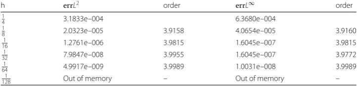
Table 1 The comparison of thel2-norm and thel∞-norm whenτ2=h
x=hyforO(h4x+h4y) fourth-order compact finite difference schemes in Example1, at different values of the step size (for
N= 4, 8, 16, 32, 64, 128) in thexandydirections
h errL2 order errL∞ order
1
4 3.1833e–004 6.3680e–004
1
8 2.0323e–005 3.9158 4.0654e–005 3.9160
1
16 1.2761e–006 3.9815 1.6045e–007 3.9815
1
32 7.9847e–008 3.9955 1.6045e–007 3.9772
1
64 4.9917e–009 3.9989 1.0031e–008 3.9989
1
128 Out of memory – Out of memory –
Example1 In this part, we study the following two-dimensional convection–diffusion equation, and give main results for the numerical approximation:
⎧ ⎪ ⎪ ⎨ ⎪ ⎪ ⎩
∂C
∂t =Dx
∂2C
∂x2 +Dy∂ 2C
∂y2 –v∂∂Cx +f, (x,y)∈,t> 0,
C(x,y,t) =g(x,y,t), (x,y)∈,t> 0,
C(x,y, 0) =C0(x,y), (x,y)∈.
(39)
Let the right item
f(x,y,t) =e–t2π2– 1sinπxsinπy+vπcosπxsinπy, (40)
and the exact solution of Eqs. (39),
C(x,y,t) =e–tsinπxsinπy, (41)
and we take the temporal range t ∈[0,T], Dx =Dy=v= 1 in the experiment. Here C(x,y,t) = 0, for all (x,y)∈, butf(x,y,t)= 0, for any (x,y)∈.
The spatial step size chosen in the numerical experiment are differenth=14,h=18,h= 1
16,h= 1 32,h=
1
64, andh= 1
128, respectively. Applying the numerical scheme in Sect.2to Eqs. (39), the error and convergence order of difference approximation schemes are shown in Table1(whereh=hx=hy).
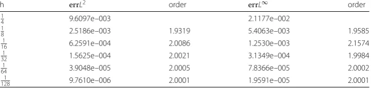
Table1demonstrates thel2-norm and thel∞-norm between numerical solution and exact solution in the case of the temporal increment is the same as the spatial increment, i.e.τ2=h. Besides, we notice that whenhis ever more smaller, the accuracy of the scheme (19) grows close to fourth order. Nevertheless, it only reaches two orders with standard difference scheme; see Table2(whereh=hx=hy).
From the above two tables, it is obvious that withN increasing, the accuracies ofl2 -norm and the l∞-norm are decreasing, that is to say, we can adopt a small spatial step size to solve this class of equation if we need the error filled with high accuracy. But for our high accuracy scheme, whenh= 1
128, the space grid involves 128×128 points; at the same time, the number of time layers is 128×128 layers, too. Due to the limitations of computer storage performance, we cannot run the results needed, we have the MATLAB display: Out of memory. For a standard general scheme, whenh= 1
Table 2 The comparison of thel2-norm and thel∞-norm whenτ=h
x=hyforO(h2x+h2y) standard central difference scheme, at different values of the step size (forN= 4, 8, 16, 32, 64, 128) in thexandy
directions
h errL2 order errL∞ order
1
4 9.6097e–003 2.1177e–002
1
8 2.5186e–003 1.9319 5.4063e–003 1.9585
1
16 6.2591e–004 2.0086 1.2530e–003 2.1574
1
32 1.5625e–004 2.0021 3.1349e–004 1.9984
1
64 3.9048e–005 2.0005 7.8366e–005 2.0002
1
128 9.7610e–006 2.0001 1.9591e–005 2.0001
Figure 2 L2-norm errors of the standard difference scheme and the compact difference scheme in
Example1. (a) Approximation order of C inL2-norm. (b)L2-norm varying with spatial step
To further collaborate the applicability of the proposed method, we have clearer pictures of the convergence of the compact difference (19), which are plotted in Fig.2, the errors in the semi-log scale, which indicates an exponential convergence rateO(τ2+h4
x+h4y) under the standard of thel2-norm and thel∞-norm, respectively.
It should be realized that the scheme (19) provides reasonable approximations of the solution in terms of the standard difference scheme. In general, Figs.2also show the fact that the present method is computationally stable, effective, simple to use, convergent and giving an accuracy of the solution better than some previously existing methods.
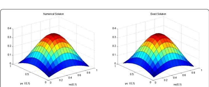
Figures3,4and5, obtained by MATLAB software, show comparison results and the changes of numerical solution and exact solution with our compact difference scheme (19) under the condition of different step sizes, both spatially and temporally.
Example2 The equation with homogeneous Dirichlet boundary condition to be solved is
⎧ ⎪ ⎪ ⎪ ⎪ ⎪ ⎪ ⎪ ⎪ ⎨ ⎪ ⎪ ⎪ ⎪ ⎪ ⎪ ⎪ ⎪ ⎩
∂C
∂t –Dx
∂2C
∂x2 –Dy∂ 2C
∂y2 +v
∂C
∂x
=e–t[–x(1 –x)y(1 –y) + 2x(1 –x)y(1 –y)
+v(1 – 2x)y(1 –y)], (x,y)∈,t> 0,
C(x,y,t) =g(x,y,t), (x,y)∈,t> 0,
C(x,y, 0) =C0(x,y), (x,y)∈.
Figure 3The effect of numerical solution and exact solution at fixedT= 1,h=14andτ=161 in Example1. (a)N= 22. (b)N= 22
Figure 4The effect of numerical solution and exact solution at fixedT= 1,h=1 8andτ=
1
64in Example1.
(a)N= 24. (b)N= 24
Figure 5The effect of numerical solution and exact solution at fixedT= 1,h=321 andτ=10241 in Example1. (a)N= 25. (b)N= 25
The exact solution of Eqs. (42) is
C(x,y,t) =e–tx(1 –x)y(1 –y)).
Table 3 The comparison of thel2-norm and thel∞-norm whenτ2=h
x=hyforO(h4x+h4y) fourth-order compact finite difference schemes in Example2, at different values of the step size (for
N= 4, 8, 16, 32, 64, 128) in thexandydirections
h errL2 order errL∞ order
1
4 6.1733e–006 1.1640e–005
1
8 3.8740e–007 3.9838 7.2789e–007 3.9979
1
16 2.4219e–008 3.9990 4.5494e–008 3.9999
1
32 1.5137e–009 3.9999 2.8434e–009 4.0000
1
64 9.4606e–0011 4.0000 1.7771e–0010 4.0000
1
128 Out of memory – Out of memory –
Table 4 The comparison of thel2-norm and thel∞-norm whenτ=hx=hyforO(h2x+h2y) standard central difference scheme, at different values of the step size (forN= 4, 8, 16, 32, 64, 128) in thexandy
directions
h errL2 order errL∞ order
1
4 3.3066e–006 1.6733e–003
1
8 8.6085e–007 1.9415 2.2786e–004 3.6718
1
16 2.1334e–007 2.0126 5.3554e–005 2.1274
1
32 5.3216e–008 2.0032 1.3026e–005 2.0556
1
64 1.3297e–008 2.0008 3.2316e–006 2.0154
1
128 3.3241e–009 2.0000 8.0609e–007 2.0045
Figure 6The effect of numerical solution and exact solution at fixedT= 1,h=321 andτ=10241 in Example2. (a)N= 24. (b)N= 24
The spatial step sizes chosen are the same as the former experiment, using the scheme (19) to Eqs. (42), we get the error and convergence order of the difference approximation schemes; see Table3(whereh=hx=hy).
Next, we give the numerical results of the standard different scheme obtained by com-puter experiment; see Table4(whereh=hx=hy).
Figure 7The effect of numerical solution and exact solution at fixedT= 1,h=641 andτ=40961 in Example2. (a)N= 26. (b)N= 26
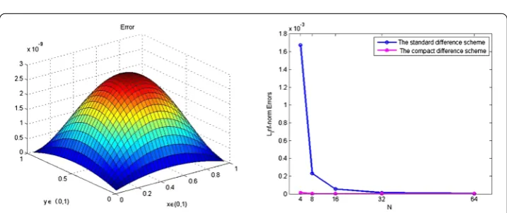
Figure 8Comparison figures of errors between the standard difference scheme and the compact difference scheme in Example2. (a) Absolute error whenT= 1,N= 32 andK=N2. (b)l∞-norm varying with spatial step
Using MATLAB, we can derive Fig.8. The left one is the picture of the absolute error by employing a fourth-order finite difference scheme. The other one is for the error curves of thel∞-norm varying with spatial step. It proves that the degree of the numerical solutions is approximating the exact solutions in different grid points.
Example3 Consider the convection–diffusion equation with non-homogeneous Dirich-let boundary condition
⎧ ⎪ ⎪ ⎪ ⎪ ⎪ ⎪ ⎪ ⎪ ⎨ ⎪ ⎪ ⎪ ⎪ ⎪ ⎪ ⎪ ⎪ ⎩
∂C
∂t –Dx
∂2C
∂x2 –Dy∂ 2C
∂y2 +v
∂C
∂x
= (2π2– 1)e–tsinπxcosπy+πe–tcosπxcosπy, (x,y)∈,t> 0,
C(x,y,t) =g(x,y,t), (x,y)∈,t> 0,
C(x,y, 0) =C0(x,y), (x,y)∈.
(43)
The exact solution of this problem (43) given by
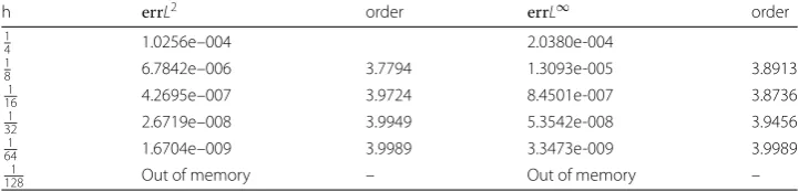
Table 5 The comparison of thel2-norm and thel∞-norm whenτ2=h
x=hyforO(h4x+h4y) fourth-order compact finite difference schemes in Example3, at different values of the step size (for
N= 4, 8, 16, 32, 64, 128) in thexandydirections
h errL2 order errL∞ order
1
4 1.0256e–004 2.0380e-004
1
8 6.7842e–006 3.7794 1.3093e-005 3.8913
1
16 4.2695e–007 3.9724 8.4501e-007 3.8736
1
32 2.6719e–008 3.9949 5.3542e-008 3.9456
1
64 1.6704e–009 3.9989 3.3473e-009 3.9989
1
128 Out of memory – Out of memory –
Table 6 The comparison of thel2-norm and thel∞-norm whenτ=hx=hyforO(h2x+h2y) standard central difference scheme, at different values of the step size (forN= 4, 8, 16, 32, 64, 128) in thexandy
directions
h errL2 order errL∞ order
1
4 1.4022e–003 4.4825e–002
1
8 8.2045e–004 0.7733 3.1211e–003 14.3618
1
16 2.0868e–004 1.9751 1.5901e–003 1.9628
1
32 5.2198e–005 1.9992 1.1661e–003 1.3637
1
64 1.3050e–005 1.9999 6.8089e–004 1.7126
1
128 3.2626e–006 2.0000 3.6604e–004 1.8601
Taking the temporal ranget∈[0,T] still, the coefficients are chosen asDx=Dy= 1,v= 1. We use this problem to check the accuracy for two different schemes: the scheme (19): the fourth-order compact finite difference scheme and the standard scheme: the second-order centered difference scheme.
Choosing the same time step sizes as the former ones, we show in Table4the errors inl2 -norm and thel∞-norm for scheme (19) to Eqs. (43) with different grid points, meanwhile, we also give the error and convergence order of standard second-order difference schemes; see Table6.
From Table5and Table6, whenT= 1, in the sense of either thel2-norm or the l∞ -norm, we can see that second-order standard finite difference scheme is worse than the proposed fourth-order compact finite difference scheme (19). Especially, whenN= 22, the convergence order of standard second-order difference schemes is obviously not in conformity with the theoretical results. In addition, with the increase ofN, although the
l2-norm gradually converges to second order, for thel∞-norm, the numerical results are not very satisfactory, it produces a slight fluctuation with the increase ofN. Compared with this, our method is more accurate and shows good convergence; it yields the smallest errors among the two methods.
Applying MATLAB software, we get the numerical solution compared with exact solu-tion as shown in Figs.9,10and11, these three pictures show the corresponding compu-tational simulation results with varying number of mesh gridN.
Figure12shows the absolute error of the scheme (19) for the fixed number ofN, and it describes the order between the two difference methods.
Figure 9The effect of numerical solution and exact solution at fixedT= 1,h=1 4andτ=
1
16in Example3.
(a)N= 22. (b)N= 22
Figure 10 The effect of numerical solution and exact solution at fixedT= 1,h=18andτ=641 in Example3. (a)N= 23. (b)N= 23
Figure 11 The effect of numerical solution and exact solution at fixedT= 1,h= 1 64andτ=
1 4096in
Example3. (a)N= 26. (b)N= 26
Figure 12 Comparison figures of errors between the standard difference scheme and the compact difference scheme in Example3. (a) Absolute error whenT= 1,N= 32 andK=N2. (b) Approximation order of
CinL2-norm
6 Conclusions
Compact finite difference schemes up to order four for solving the convection–diffusion equation in two dimensions were developed in this paper. To further collaborate the appli-cability of the proposed method, tables of thel2-norm and thel∞-norm forO(τ2+h4
x+h4y) compact finite difference schemes and corresponding graphs have been plotted for Exam-ples1,2and3, for the exact solution versus the numerical solutions at different values of mesh sizeh. It is found that not only the error norml2decreases with the increase of the number of nodes but also thel∞-norm shows the same trend; it decreases as the mesh sizehdecreases, which in turn shows the convergence of the computed solution. To sum up, the present method is computationally stable, effective, simple to use, convergent and giving a better accuracy of the solution than some previously existing methods.
Acknowledgements
The authors are very grateful to Xu Qiang of Shandong Normal University, Qiao Haili of Shandong University and Wang Xuanxin of Jinan University for their help and suggestions in the process of numerical calculation. We are also very grateful to the reviewers for their valuable comments.
Funding
This work is supported by National Natural Science Foundation of China (Nos. 11501335, 11371229), the Natural Science Foundation of Shandong Province of China (No. ZR2017MA020), and the Project of Shandong Province Higher Educational Science and Technology Program (No. J14LI03).
Availability of data and materials Not applicable.
Competing interests
The authors declare that they have no competing interests.
Authors’ contributions
LL carried out the main part of this article. All authors read and approved the final manuscript.
Publisher’s Note
Springer Nature remains neutral with regard to jurisdictional claims in published maps and institutional affiliations.
Received: 7 March 2018 Accepted: 30 May 2018
References
1. Zhu, Q., Wang, Q., Fu, J., Zhang, Z.: New second-order finite difference scheme for the problem of contaminant in groundwater flow. J. Appl. Math.2012(2012), 129–154 (2012)
3. Li, L.Y., Yin, Z.: Numerical simulation of groundwater pollution problems based on convection–diffusion equation. Am. J. Comput. Math.7(3), 350–370 (2017)
4. Saqib, M., Hasnain, S., Mashat, D.S.: Computational solutions of two dimensional convection–diffusion equation using Crank–Nicolson and time efficient ADI. Am. J. Comput. Math.7(3), 208–227 (2017)
5. Mekuria, G.T., Rao, J.A.: Adaptive finite element method for steady convection–diffusion equation. Am. J. Comput. Math.6(3), 275–285 (2016)
6. Qiu, W., Shi, K.: An HDG method for convection–diffusion equation. J. Sci. Comput.66(1), 346–357 (2016) 7. Shu, C.W.: Bound-preserving high order finite volume schemes for conservation laws and convection–diffusion
equations. In: Finite Volumes for Complex Applications VIII—Methods and Theoretical Aspects, Springer Proceedings, pp. 3–14 (2017)
8. Ammi, M.R.S., Jamiai, I.: Finite difference and Legendre spectral method for a time-fractional diffusion-convection equation for image restoration. Discrete Contin. Dyn. Syst.11(1), 103–117 (2017)
9. Koley, U., Risebro, N.H., Schwab, C., et al.: A multilevel Monte Carlo finite difference method for random scalar degenerate convection–diffusion equations. J. Hyperbolic Differ. Equ.14(3), 415–454 (2017)
10. Noye, B.J., Tan, H.H.: Finite difference methods for solving the two-dimensional advection–diffusion equation. Int. J. Numer. Methods Fluids9(1), 75–98 (1989)
11. Lu, J.F., Guan, Z.: Numerical Methods for Partial Differential Equations. Qinghua University Press, Beijing (2003) 12. Sun, Z.Z.: Numerical Methods for Partial Differential Equations. Science Press, Beijing (2005)
13. Zhang, J.: An explicit fourth-order compact finite difference scheme for three-dimensional convection–diffusion equation. Int. J. Numer. Methods Biomed. Eng.14(3), 209–218 (2010)
14. Sari, M., Gürarslan, G., Zeytino ˇglu, A.: High-order finite difference schemes for solving the advection–diffusion equation. Math. Comput. Appl.15(15), 449–460 (2010)
15. Qiao, H.L., Jiang, Z.W.: The high accuracy compact finite difference scheme for three dimensional convection–diffusion equation. J. Shandong Univ. Nat. Sci.1(32), 6–9 (2017)
16. Gurarslan, G., Karahan, H., Alkaya, D., et al.: Numerical solution of advection–diffusion equation using a sixth-order compact finite difference method. Math. Probl. Eng.2013(3), 532–546 (2013)
17. Singer, I., Turkel, E.: High-order finite difference methods for the Helmholtz equation. Comput. Methods Appl. Mech. Eng.163(1–4), 343–358 (1998)
18. Bullo, T.A.: Fourth order compact finite difference method for solving one dimensional wave equation. J. Comput. Appl. Math.8(4), 30–39 (2016)
19. Cui, M.R.: Compact finite difference method for the fractional diffusion equation. J. Comput. Appl. Phys.228(20), 7792–7804 (2009)
20. Tian, Z.F., Ge, Y.B.: A fourth-order compact ADI method for solving two-dimensional unsteady convection–diffusion problems. J. Comput. Appl. Math.198(1) 268–286 (2007)
21. Li, Y.B., Kim, J.: An efficient and stable compact fourth-order finite difference scheme for the phase field crystal equation. Comput. Methods Appl. Mech. Eng.319, 194–216 (2017)
22. Kaysar, R., Arzigul, Y., Zulpiya, R.: High-order compact finite difference scheme for solving one dimensional convection–diffusion equation. J. Jiamusi Univ. (Nat. Sci. Ed.)1(32), 135–138 (2014)
23. Sun, N.Z.: Groundwater Pollution: Mathematical Models and Numerical Methods. Geological Press, China (1989) 24. Yang, X.J., Wang, Y.: High accuracy explicit compact difference scheme for the diffusion equation. J. Hebei Univ. (Nat.
Sci. Ed.)2(36), 117–123 (2016)
25. Tian, Z.F., Dai, S.Q.: High-order exponential finite difference methods for convection–diffusion type problems. J. Comput. Phys.220(2), 952–974 (2007)
26. Tian, Z.F., Cui, J.: A new method of constructing fourth-order compact scheme for the steady convection–diffusion equation. In: Zhuang, F.G. (ed.) Proceeding 7th International Symposium on Computational Fluid Dynamics, vol. 2, pp. 116–121. International Academic Publishers, Beijing (1997)
27. Ames, W.F.: Numerical Methods for Partial Differential Equations. Academic Press, New York (1977) 28. Li, R.H., Liu, B.: Numerical Methods for Partial Differential Equations. Higher Education Press, Beijing (2008)
29. Liu, M.H.: High-order compact difference method for the 2-D Poisson equation. J. Fujian U. Tech.4(3), 373–376 (2006) 30. Zapata, M.U., Balam, R.I.: High-order implicit finite difference schemes for the two-dimensional Poisson equation.