R E S E A R C H
Open Access
A distributed multi-robot adaptive sampling
scheme for the estimation of the spatial
distribution in widespread fields
Muhammad F Mysorewala
1*, Lahouari Cheded
1and Dan O Popa
2Abstract
Monitoring widespread environmental fields is undoubtedly a practically important area of research with many complex and challenging tasks. It involves the building of models of the fields or natural phenomena to be monitored, the estimation of the spatio-temporal distribution of a variety of environmental parameters of interest, such as moisture or salinity in a crop field, or the spatial distribution of vital natural resources such as oil and gas, etc. Sampling, a key operation of the monitoring process, is a broad methodology for gathering statistical
information about the phenomenon, or environmental variable, being monitored. To efficiently monitor widespread fields and estimate the spatio-temporal distribution of some particular environmental variable, calls for the use of a sampling strategy can fuse information from different scales of sensors. Such an attractive strategy is well catered for by both the capabilities and distributed nature of wireless sensor networks and the mobility of robots performing the sampling (sensing) tasks. This sampling strategy could even be rendered“adaptive”in that the decision of“where to sample next”evolves temporally with past measurements and is optimally computed. In this article, we examine various single-robot and multi-robot adaptive sampling schemes based on different extended Kalman filter filtering structures such as centralized and decentralized filters as well as our own novel decentralized and distributed filters. Our investigation shows that, whereas the first two filters suffer from a heavy computational or communication load, our proposed method, through its key feature of distributing the filtering task amongst the robots used, manages to reduce both loads and the total reconstruction time. It also enjoys the added attractive feature of scalability that allows the structure of the proposed monitoring scheme to grow with the complexity of the field under study. Our results are corroborated by our simulation work and offer ample encouragement for a further theoretical investigation of some properties of the proposed scheme and its implementation on a physical system. Both of these activities are currently underway.
Keywords:Spatial field estimation, Adaptive sampling, Information fusion, Multi-scale sensing, Robotic sensor network, Environmental monitoring
Introduction
Mobile robots are being increasingly used as sensor-carrying agents to perform sampling missions, such as searching for harmful biological and chemical agents, search and rescue in disaster areas, and environmental mapping and monitoring. One of the objectives of these sampling missions is ‘Field Estimation’. Field estimation is the construction of an estimate of how a certain
parameter varies in space and time, i.e., an estimate of its spatio-temporal distribution, based on observed or sampled data. As the field of interest is spread over a wide area, using a dense and fixed sampling scheme for an efficient field mapping would simply be too costly and will involve a possibly prohibitive computational load. Instead, it is far more interesting to use a mobile sampling scheme that would collect samples at few judi-ciously selected locations, in a way that would enable it to gain enough information about the field to be able to infer, with significant accuracy, the value of the parameter of interest at the unsampled locations. A
* Correspondence:[email protected]
1
Systems Engineering Department, King Fahd University of Petroleum and Minerals, Dhahran 31261, Saudi Arabia
Full list of author information is available at the end of the article
multitude of research groups have published results on sampling using mobile robots for chemical plume source localization [1,2], soil–moisture mapping for crop monitoring [3], ocean sampling [4,5], forest-fire mapping [6], etc.
The sensor fusion schemes for sampling missions can broadly be classified into three categories based on (i) physical parametric models, (ii) feature-based inference techniques such as clustering algorithms, neural net-works, etc., which are generally non-parametric in na-ture but can lead to black or grey box parametric representation of the process, and (iii) cognitive-based models, which use the inference processes of humans and animals and which are based on fuzzy logic rules, search techniques, information-theoretic approaches, etc. Models acquired using these three broad classes of approaches can be either purely deterministic or purely stochastic. In many cases, deterministic models affected by some random noise can also be assumed.
In the area of physical deterministic parametric model-ing representmodel-ing the first category of samplmodel-ing missions, Christopoulos and Roumeliotis [2] presented an ap-proach for estimating the parameters of the diffusion equation that describes the propagation of an instantan-eously released gas. Cannell and Stilwell [4] presented two approaches for adaptive sampling (AS) of under-water processes using AUVs. The first one assumes a parametric model, while the second one uses an information-theoretic approach. A number of strategies for non-parametric AS can also be found in the litera-ture. A solution for non-parametric ocean sampling is proposed in [7] based on a classification of the sampling
area. The multi-robot path planning problem is
addressed in [8] using the mutual information collected using different paths. The study of [5] is also similar to that of [8] in the sense that both deal with generat-ing optimal trajectories for multiple underwater vehicles
for sampling purposes. Rule-based non-parametric
approaches are also used widely in chemical plume tracing on land and in water, odor sensing [2], mine detection, etc.
Forest fires, chemical source leaks, and temperature variations in oceans are examples of complex natural phenomena for which the exact nonlinear model descriptions are unattainable due to the high-level of complexity involved. Demetriou and Hussein [9] present a solution to the problem of estimating a spatial distri-bution when the process is described by a partial differ-ential equation. In [10], a non-parametric model is considered, and a distributed scheme for field estimation is developed using a Kalman filter-like recursive scheme.
In geostatistics, spatial processes are generally modeled as random fields, and estimation is performed using Kri-ging Interpolation techniques [11,12]. KriKri-ging is termed
“simple” if the mean of the distribution is also known, and“universal”if the mean is treated as an unknown lin-ear combination of known basis functions. In [13], a dis-tributed algorithm is presented for spatial estimation using the Kriged Kalman filter. Graham and Cortes [14] proposed a Kriged Kalman filter-based approach for a spatiotemporal field where the discrete-time evolution of the state is governed by the Kalman filter used. In [15], the authors represent the time-varying field with a ran-dom process with a covariance known up to a scaling parameter. They proposed gradient descent algorithm which can run in a distributed fashion on multiple robots. Olfati-Saber [16,17] developed a distributed Kal-man filter approach along with consensus filters to esti-mate the state of a process and reach consensus of all nodes.
Due to the time and energy-critical nature of some of these sampling scenarios, simply requiring the robots to perform a raster scan or randomly sample the field of interest would clearly be a sub-optimal and highly ineffi-cient sampling strategy. Moreover, many time-varying distributions of interest encompass a wide area, and must therefore be observed with sensors having variables characteristics such as multiple size scales, rates, and ac-curacies [18]. For example, a forest fire is monitored using satellite images which provide a large spatial field-of-view (FOV) but a low-resolution or fidelity. On the other hand, a plane flying at low altitude would provide a low-spatial FOV but high-fidelity information.
In order to effectively fuse these different types of
measurements, we proposed a Multi-scale Multi-rate
Adaptive Samplingapproach with a parametric descrip-tion of the field [6]. In this approach, sampling strategies continuously adapt in response to real-time measuments from sensors of different scales. This scheme re-lies on building parametric models of the field using spatial sensor measurements collected from a high-altitude, and which are thus less accurate, and then improving the models by using more accurate spot mea-surements. The extended Kalman filter (EKF) is used to derive a quantitative information measure that is needed for the selection of sampling locations that are mostly likely to yield optimal information. In this approach, the existing low-resolution information of the field is first used to acquire an initial parametric representation of the field whose parameters have a higher initial error co-variance which gradually reduces as high-resolution samples are taken and processed.
network (NN) for the parameterization of the non-parametric field, (b) an EKF for parameter estimation, and (c) a heuristic search scheme called ‘Greedy Adap-tive Sampling’(GAS).
A further investigation of the AS algorithm using mul-tiple robots is presented in this article. For widespread fields, it may be impractical and certainly inefficient for a single-robot to map the entire field by navigating to different sampling locations, even when guided by an ef-ficient sampling algorithm. However, when using mul-tiple robots, the sampling area is first divided into smaller regions, and then each sampling instance in a particular region gains information about the parameters which have a dominant effect in that region. Therefore, in order to distribute computations, we need to be able to fuse the parameter estimates in order to construct the map of the field density distribution.
This problem is similar to reformulating the algorithm originally designed for a conventional single-sensor sin-gle-processor system to work on a more general multi-sensor, multi-processor system. Distributed algorithms have been used before in many applications, and the de-gree of parallelism used in them varies from one algo-rithm to another, depending on the application at hand. An example of distributing processing includes target location estimation using several sensors for data collec-tion, and then fusing together the collected measure-ments either at the central station or at each sensor in a multi-sensor fusion algorithm [19-21].
Since complex fields are represented by hundreds of parameters [6], it is computationally cumbersome for a single-robot to compute and store all parameter esti-mates and the uncertainty measures. It also quickly becomes unfeasible for individual robots to run a large
AS algorithm, and share large covariance matrices wire-lessly. Furthermore, with multi-robot sampling, the resources can be allocated efficiently if some resources are either busy or not available.
If the filter computation can be distributed among multiple robots, the number of computations per-formed by all the robots, i.e., the overall computational efficiency would be greater than the processing carried out by a single-robot having to carry-out both the sam-pling and computational tasks. Moreover, we expect that the concomitant advantages such as the flexible degree of parallelism, speed of convergence, and reduc-tion in complexity that will be thus gained would be significant. With a single-robot, the total field estima-tion time includes the time necessary for navigaestima-tion, sensing, and computation of the estimate (as there is no communication involved in this case). With multiple robots, the field estimation time includes the time taken for sensing, computation, communication, and final fusion to recover the field density distribution. We expect that the speed of convergence would in-crease by using multiple robots simply because of the sampling being done in parallel, and that the navigation time would be reduced significantly at the cost of mod-est increases in computation, communication, and fusion.
The rest of the article is organized as follows: in Sec-tion 2, we present the general formulaSec-tion of the AS problem; Section 3 summarizes the existing centralized and decentralized filters, and their application to sensor network for field estimation; in Section 4, we present the novel federated distributed KF; Section 5 presents the simulation results for the proposed algorithm, and their discussion; finally Section 6 concludes the article.
Formulation of multi-robot AS algorithm
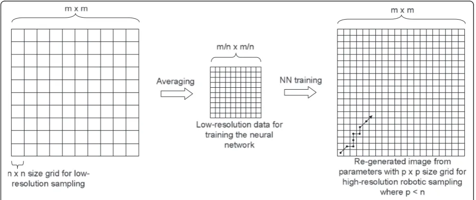
As covered in our previous study, a single-robot-based AS algorithm for a 2D spatially stationary fieldg(x,y)can be described as follows [6] (Figure 1).
(1)Low-resolution sampling: The fieldg(x,y) of size
m×mis divided into uniform square-sized grids
n×nsuch thatn<m, and samples are collected at the centers of each of then×ngrids. Hence,
m/n×m/nsamples are collected as a low-resolution representation of the actual field.
(2)Parameterization:Parametric representation of the fieldg(x,y) is achieved by training a B-neuron RBF neural network with the acquired low-resolution data. This results in a representation of the field as a sum ofBGaussians (one per neuron), and an offset (or bias) parameterb, with each neuron having its own parameters such as its peakai, varianceσi, and
centerðx0i;y0iÞ. Each of these parameters has an initial estimate valueA0, and an initial error covarianceP0. The number of neuronsBis chosen depending on the complexity of the field and in such a way that the initial field estimation error is
minimized to a value less than an acceptable threshold. Note at this stage that unlike the low-resolution samples which are uniformly distributed since they are acquired from uniformly distributed grids, the Gaussians (one Gaussian per RBF node) are distributed non-uniformly depending on the density of the field. We actually use more Gaussians in denser areas and fewer Gaussians in smoother areas of the field to be mapped. Further details on the relationship between the number of low-resolution samples and the number of neurons can be seen in [6].
Mathematically, a spatially stationary field is represented by the parameter vectorAdefined by
A¼½b a1 σ1 x01 y01 . . . aB σB
x0B y0BTk ð1Þ
whereAis the vector containing the true values of the parameters, which is not known due to (i) the resolution error between the actual field and the acquired low-resolution version, and (ii) RBF training error.
(3)High-resolution sampling:In order to improve the field estimate, spot-measurements are made by a robotic vehicle which collects samplesZkin a grid of sizep×p(wherep≤n) based on a heuristic GAS algorithm [6]. According to the GAS algorithm, the next sampling location is searched within the vicinity of the currently sampled location, based on a criterion of minimization of the norm of the parameters’error covariance matrix.
The EKF governing and measurement equations are respectively given by
whereQ is the process noise covariance,Ris the meas-urement noise covariance and (xk,yk) are the robot
sam-pling locations.
The multi-agent (or multi-robot) AS problem consid-ered here can be described as follows:
Assumptions:
(i)A nonlinear spatio-temporal field variable is described via a parametric approximation
Z = Z(A, X, t) depending on an unknown parameter vector A, position vector X, and time t.
(ii)N robotic vehicles (agents) sample the field with sensing uncertainty in order to obtain higher resolution estimates of the field.
(iii)The number of field parameters (L) and their initial guesses are based on a hypothesis originating from prior knowledge of the field consistent with a low-resolution image of the entire field.
As a complex spatial field is spread over a large area, its parameterization will require a large number of para-meters. Therefore, it becomes unfeasible for a single-robot to navigate to different locations, collect samples, and improve parameter estimates in a short period of time. In addition to time constraints, the sampling prob-lem also experiences constraints in the amount of energy available to the robot, as well as suffers from a consider-able computational burden. These constraints limited the performance of our single-robot AS algorithm as described in [22]. Therefore, a key contribution of this article is to propose a better alternative that greatly alle-viates the time and energy constraints imposed on the sampling process by the single-robot approach of map-ping a spatio-temporal stationary field.
[23], we considered the scenario with two measurements only: the field measurement and the location of the robots.
It is important at this juncture to describe the follow-ing three main issues which underline the multi-robot sampling problem tackled here.
(i) How can the sampling area be divided efficiently? Section 2.1 discusses the above issue and suggests some efficient ways of tackling it.
(ii) How can the density distribution be estimated through efficient data fusion when robots are collecting measurements in parallel?
(iii)How can the computational and communication burden be distributed efficiently amongst the many robots used?
To address the last two issues, several possible algo-rithms are first presented in Sections 3&4, and then their respective simulation results presented and dis-cussed in Section 5.
Partitioning of sampling area
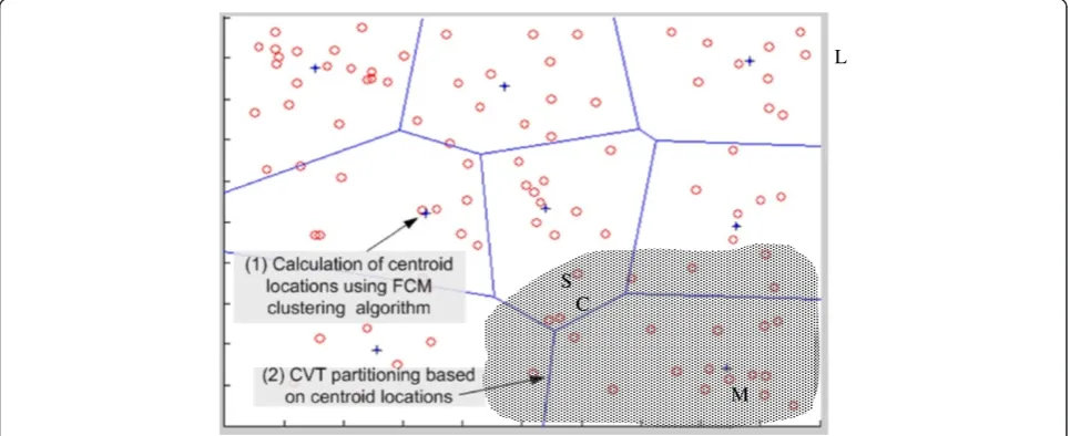
A method is clearly needed to efficiently divide the sam-pling area into clusters, in order to run a parallel AS al-gorithm with multiple robots. Here, we propose an approach to efficiently divide the sampling area for para-metric distributions using Fuzzy c-means clustering (FCM) and Centroidal Voronoi Tessellation (CVT) dia-grams.FCM has frequently been used in the past for the classification of numerical data. CVT diagrams [24] have also been used for forming non-uniform size grids to better explore high-variance areas for non-parametric distributions [7]. Here, we employ a scheme to efficiently divide the sampling areas for parametric distributions
using both FCM and CVT. In this approach, FCM clus-ters samples based on the estimated cenclus-ters of the ap-proximating Gaussians used to map the field. Note here that we have assumed that the partitioning is performed once only at the beginning of the Fusion filter. For a time-varying field, further accuracy can be obtained by re-partitioning the field (and hence repositioning the Gaussians) after some samples to account for the field evolution in time.
As discussed in the beginning of this section, low-resolution samples fromg(x,y) are used to train the RBF neural network which gives an estimate of the field as a sum ofB Gaussians (neurons). This clustering approach is illustrated in Figure 2, where a field represented by B= 100 Gaussians is partitioned into eight regions. The centers of these Gaussians shown in red circles are used for clustering.
As the clustering is fuzzy, it allows one piece of data to belong to several clusters via a membership grade u ranging between 0 and 1, and involves the iterative minimization of the cost function [25] given in Equation (3).
Jm¼ XL
i¼1 XN
j¼1
umijxicj 2
;1≤m<1; ð3Þ
where L¼4Bþ1 is the number of Gaussian centers,N is the number of clusters which is equal to the number of robots in this case,uijis the degree of membership of
center xi in cluster j, cj is the centroid of the cluster j
andmis a real number greater than 1. Next, a CVT dia-gram based on Lloyd’s algorithm uses the centroid loca-tions acquired by fuzzy clustering to classify all points in discrete space that are closest to the centroid, as a single
group. Mathematically, given C clusters, each with a
L
M C
S
centroid denoted bycs, then a pointpon the field is said
to be part of the cluster r if the following distance in-equality is satisfied:jpcrj≤jpcsj;s¼1;. . .;N;s6¼r.
As a result of this mapping scheme, more Gaussians will overlap in areas where there are large field varia-tions. The use of FCM and the CVT diagram for area classification may result in regions which have more var-iations and which must be as small as required in order to sample them thoroughly, i.e., so as not to miss out on any vital information. The areas with less variation, though they may be large, would require fewer samples, since they are represented by only a few parameters.
Centralized, completely decentralized, and federated decentralized filters
In this section, we first examine completely centralized, completely decentralized, and federated decentralized fil-ters, and their use in running the proposed multi-robot AS algorithm. We then argue that a new and efficient fil-ter is needed for this application which will be discussed in detail in the following section.
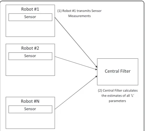
Using completely centralized filter
In a completely centralized sampling approach, each robot j¼1;2;. . .;N takes sensor measurement Zj;kþ1 and transmits them to the central processor, which then calculates the required parameter estimates A^kþ1 and error covariances Pkþ1. The central processor computes these estimates, shown below in (4), using the‘KF equa-tions for a single robot’, (while single-handedly) taking on the task of fusing the multiple measurements it acquires from theNrobots used.
Figure 3 illustrates the completely centralized ap-proach, in which all robots transmit their sensor meas-urement to the central filter, which then calculates the field estimate using Equation (4) given below where the superscript ‘-‘ in the vector A and matrix P indicates pre-measurement, while the lack of it indicates post-measurement:
EKF Pre-measurement updateða priori estimateÞ equations :
EKF Post-Measurement updateða posterior estimateÞ equations :
Here we assume a stationary field and hence time pre-diction is not needed, i.e., the a priori estimates will be ^
Akþ1¼A^k and Pkþ1¼Pk. In [6], we assumed a slow time-varying field, a single sampling robot was used, and we included the prediction too considering the time evo-lution of the field.
This type of scheme is simple, as there is little com-munication involved and no redundant computations. But, the disadvantage is that the sensing robots do not carry any information on the field to be estimated. Therefore, this algorithm cannot be adaptive for every sample because the latest estimates are required to gen-erate new sampling locations, and these estimates are Figure 3Completely centralized filter for multi-robot AS
not calculated at every robot. Simulation results are shown in Section 5, where multiple sampling locations are chosen based on the current field estimate, and then all the measurement data collected are transmitted to the central filter for fusion, further processing and deter-mination of the next sampling locations.
Using completely decentralized filter
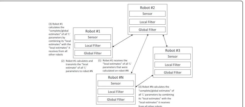
For a completely decentralized filter implementation, each robot not only takes the sensor measurement, but also runs locally the AS algorithm. However, it only cal-culates partial estimates of the field parameters and error covariance. It also generates new sampling loca-tions within the vicinity of its current position. After every few samples, the robots communicate and share with each other their partial field estimate information, in order to calculate the complete estimates. The par-ameter estimate vector and the error covariance are the two terms each robot needs to transmit to the other robots. Each robot assimilates the received information using a decentralized EKF scheme formulated in [19,26].
Figure 4 illustrates the completely decentralized filter structure in which each robot has its own filter to com-pute partial estimates, and a fusion filter for assimilating the estimates acquired from other nodes to generate the complete field estimate.
If a completely decentralized approach is considered, then an AS algorithm running on each robot carries the information about all the field parameters, and thus there is no need at all for a global fusion filter in this case. Hence, each robot j can calculate the partial or
Local Estimate (LE), A^j;kþ1;LE and Pj;kþ1;LEafter (k+ 1)th using Equation (5)
Pj;kþ1;LE ¼ Pj;k;LE1 þGTj;k;LER1Gj;k;LE
h i1
^
Aj;kþ1;LE ¼A^j;k;LE
þPj;k;LEGTj;kR1Zj;kþ1gj;k;LEðA^j;k;LEÞ where;
^
Aj;k;LE ¼ ^b0;k ^a1;k σ^1;k ^x01;k ^y01;k . . . ^aB;k
h
^
σB;k ^x0B;k ^y0B;k iT
j;LE
gj;k;LEA^j;k;LE¼^b0;j;k;LE
þXB
i¼1 ^
ai;j;k;LEexp ð
x^x0i;j;k;LEÞ2þðy^y0i;j;k;LEÞ2 2σ^2i;j;k;LE
( )
Gj;k;LE ¼ @gk
@^b0;k
@gk
@a^1;k
@gk
@σ^1;k
@gk
@^x01;k
@gk
@^y01;k "
. . . @gk
@^aB;k
@gk
@σ^B;k
@gk
@^x0B;k
@gk
@^y0B;k #T
j;LE
ð5Þ
Note that Gj,k,LE, where j, k, LE stand for the sensor
number, sample number, and LE, respectively, is the Jacobian of the Gaussian vectorgj,k,LE, and is used in the
above linearized EKF measurement update equation to estimateA^j;k;LE.
To compute the rthupdate, robotjcalculates the total estimate ðA^j;r;Pj;rÞafter each robot has collected its own
q samples as explained next. First it (robot j) acquires from the other robots their new partial estimates
ðA^i;rq;LE;Pi;rq;LEÞwhich were computed fromqnew
sam-ples and then assimilates these new partial estimates
with both its previous total estimates ðA^j;r1Pj;r1Þand
its own new partial estimates. The complete rth
updates, Pj,r and A^j;r, are finally computed by robot j
using Equation (6) [19]:
ðPj;rÞ1¼ðPj;r1Þ1þ XN
i¼1
ðPi;rq;LEÞ1 ðPi;ðr1Þq;LEÞ1
^
Aj;r¼Pj;r ðPj;r1Þ1A^j;r1þ XN
i¼1
ðPi;rq;LEÞ1A^i;rq;LE
"
ðPi;ðr1Þq;LEÞ1A^i;ðr1Þq;LE
#
ð6Þ The advantage of this approach is that it does not in-volve any approximations, and there is no dependence on a central filter for computing the partial estimates. Also, the objective of sampling in parallel can be suc-cessfully achieved. The disadvantage of the algorithm is that it is demanding and inefficient in terms of commu-nication and computational requirements when there are many parameters to estimate and heavy communica-tion requirements to satisfy. This network has to be fully connected and there is excessive communication. This full parallelism (and complete distribution) of this type of algorithm can be taken advantage of in applications such as target tracking which involve the estimation of a few parameters (such as location, speed, etc., of the
target) only. When a large number of parameters are to be estimated, dividing the entire field of interest into several sampling areas and provided a sufficient number of robots is allocated to each area, then there will be no doubt that, through communication, this will enable dif-ferent robots to carry better information about difdif-ferent parameters, thus resulting in an improvement of the overall estimation of the field. If only a few robots are used to sample a particular area, then each robot will have a larger sampling area to cover and it will take more time to calculate the local parameter estimates up to a certain degree of accuracy, from which it will then calculate the global estimate of the field parameters. This may not be possible under time constraint. This is clearly illustrated in Table 1 where reduction in number of robots from 4 to 1 resulted in an almost four fold in-crease in the total sampling time.
By the way of example, in adaptively sampling a field (shown in Figure 2) represented by B= 401 parameters. The field is divided into N= 8 partitions and the sam-pling operation is performed using 1 robot/partition. Running this decentralized algorithm would require each robot to calculate the partial estimate of 401 parameters, and to wirelessly transmit an error covariance matrix of size 401 × 401, and a parameter estimate vector of size 401 × 1 to every other robot. Clearly, such a scheme would be very inefficient and not scalable.
Table 1 Comparison of simulation results for single robot, multi-robot decentralized and federated decentralized filter
Single-robot Multi-robot centralized KF (non-AS)
Multi-robot decentralized federated and
non-federated fusion
Field size (m×m) 300 × 300 300 × 300 300 × 300
Grid size for initial samples collection (n×n) 30 × 30 30 × 30 30 × 30
Number of neurons (B) 40 40 40
RBF variances (σ) 30 30 30
Number of sampling robots (N) 1 4 4
Grid size for adaptive sampling (p×p) 5 × 5 5 × 5 5 × 5
Horizon size (in grids) for next sample selection for each robot 10 30 10
Initial parameters error covariances b ai siix0iy0i
200 50 107 4 4
200 50 107 4 4
200 50 107 4 4
Sensor measurement error covariance (R) 1 1 1
Initial norm of error covariance of all parametersðk kÞP0 375.9 375.9 375.9
Final norm of error covariance of all parametersðkPkþ1kÞ 13.25 241.0 17.27
Norm of error between original and initial estimated fieldðkggest0kÞ
25.05 25.05 25.05
Norm of error between original and final estimated fieldðE2F¼kggestkþ1kÞ
19.67 48.0 19.33
Time taken to reachðkggestkþ1kÞ<20 11.92 min 5.48 min 2.89 min
No. of samples (qN) 300 300 320
No. of times KF runs for calculating the parameter estimates 300 (complete estimate) 1 (complete estimate) 320 (partial estimate)
# of samples/robot after which global estimate is calculated (q/r) 1 300 20
Using a federated decentralized filter
In this approach, each robot takes some sensor measure-ments, estimates partial error covariances and field para-meters, and transmits this information to a global fusion filter for assimilation, in a similar fashion to the ap-proach proposed in [20,21,27]. Each robot runs Equation (5), but the fusion is done only at the fusion filter using Equation (6). Then these estimates are transmitted by the global fusion center (or filter) to all of the robots. So, the only difference between federated and completely decentralized approach is that in the federated case, these estimates are centrally calculated by the common global fusion filter while in complete decentralization, these are locally estimated at each robot.
Figure 5 illustrates the federated decentralized filter in which each robot calculates partial field estimates, and transmits them to the global fusion filter, which then computes the complete field estimates. The advantage of this approach is that there is less communication com-pared to the completely decentralized case. Although in this case, none of the robots carries the complete infor-mation about all of the parameters all of the time, this approach will also be computationally more efficient than the completely decentralized implementation, sim-ply because of the removal of the computational redun-dancy, due to fusion taking place at every robot, that was needed in the completely decentralized scheme. The disadvantage that this approach shares with the com-pletely decentralized one is that partial estimates of all
parameters are still being carried by all of the robots all of the time, although information about these estimates might not be complete. Therefore, by federating the decentralized KF filtering scheme, the computational as-pect of the problem has been mitigated but not the com-munication one. A thorough examination of the above three filtering schemes has therefore led us to take a novel and fruitful approach that would reduce both computational and communication overheads simultan-eously. This novel approach is underpinned by a shift in focus from the mere decentralization of the KF filter to its distribution as described in the following section.
Federated distributed Kalman filter
A decentralized and a distributed KF are two different for-mulations of the same KF algorithm [19]. In a decentra-lized algorithm, the filter is full-order, which means that every local filter carries partial information about all para-meters, and the information is shared in a star topology to reach consensus amongst all robots on the final parameter estimates. The objective of distributed algorithms is to effi-ciently decompose the full-order filter into several reduced-order filters, in order to reduce the computational complexity and communication overhead, and hence im-prove the scalability. It can be said that decentralization is the first step toward efficient distribution. In case of no distribution, every collected sample is used to compute the estimates of all parameters in the field. But with distribu-tion, this sample is used to compute the estimates of only those parameters which have significant impact on the re-gion where this sample has been collected.
The objective of the work presented in this section is to modify the formulation of a federated decentralized scheme, in order to reduce both the communication overheads and the computational load involved. This formulation considers only the cross-covariance terms contributed by neighboring Gaussians only and ignores those contributed by distant Gaussians as a trade-off be-tween accuracy and computational complexity. The de-cision behind ignoring distant Gaussians is supported by the analysis provided in Section 5, where a threshold of 0.001% in the relative contribution of each Gaussian was used in deciding the number of Gaussians to keep. An accurate DKF is not possible in this AS problem because local measurement models are not available. Further-more, the use of global measurement models at each node requires the estimate of all parameters, which will contradict the motivation behind the implementation of DKF. There are other schemes that handle the error co-variance terms“very lightly”such as Kalman Consensus schemes, which take the average of the error covariances of the parameter estimates in order to implement the DKF with only communication between neighboring nodes being used [16,17].
Decentralized approaches are good enough for appli-cations involving a small number of states such as track-ing of objects, etc. But problems such as parametric sampling involve hundreds of parameters, and hence distributing the KF filter becomes all the more important for an efficient operation.
Approach to distributed computations and communications
Assume that we have a continuous field distribution within a certain perimeter, which means that there is dis-continuity between the field and its surroundings. As shown in Figure 2, this field is represented by L para-meters, whereL¼4Bþ1, and the field estimate is calcu-lated at the central station based on the LEs received
from Nsampling robots. In the example shown in
Fig-ure 2,B= 100, N= 8, and L= 401. The circles shown are the centerðx0i;y0iÞofBGaussians. One of the highlighted partitions has S parameters, the estimates of which are expected to change by collecting samples from that parti-tion. S includes all the parameters inside a partition, as well as the surrounding parameters which have a signifi-cant impact on that partition. The collection of a single
sample leads to the change in M parameter estimates,
whereas collecting multiple samples results in the change
of C parameter estimates. Hence, from a set-theoretic
point of view, we can state thatM⊂C⊂S⊂L.For the decen-tralized case, M=C=S=L and all the cross-covariance terms contributed by all the Gaussians are considered. However, for the distributed case, we haveM⊂C⊂S⊂Land an increase in M,C, andSwill lead to a better accuracy at the cost of a higher number of computations.
The idea behind this approach is to run a reduced-order KF rather than a full-reduced-order one so as to reduce the computational load, as well as the communication over-heads by transmitting only the smallest amount of infor-mation needed.
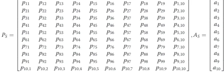
Given the following sizes of the variables involved: ^
AM2RMx1;PM 2RMxM;A^C 2RCx1;PC2RCxC;A^S2 RSx1;
PS2RSxS;A^L2RLx1;PL2RLxL, this approach in-volve the following steps:
1. Transformation fromðPL;;AL^ ÞtoðPS;AS^ Þat the
fusion filter.
The fusion filter evaluates the initial estimate of
ðPS;AS^ Þby first generating the binary
transformation matrixULS(to transformLtoS), and transmittingðPS;AS^ Þto robot 1. The matrix
ULS¼USLT is kept in memory by the fusion filter for
the final assimilation stage.
PS¼ULSTPLULS;AS^ ¼ULSTAL^
3. Collect the measurement- and estimate pair,
ðPM;kþ1;AM^ ;kþ1Þ sample, and the transformation ofCfromkthto (k+ 1)thsample, respectively.
5. Repeat steps3 and 4 until an update is requested from the fusion filter.
6. Transmit the pairðPC;A^CÞto the fusion filter
8. The fusion filter finally runs the global update Equation (6) considering all the different pairs
ðPj;L;LE;A^j;L;LEÞto be local updates from different
For clarification, an example is shown below withL= 401,S= 10,C= 5,M= 3 (for two samples). respectively, estimate the parameters (2,4,7), (3,4,6), and (1,2,4,9). Then,
For the first sample: parameters (2, 4, 7) changes. Therefore,
For the second sample: parameters (3, 4, 6) changes. Therefore,
For the third sample parameters (1, 2, 4, 9) changes. Therefore,
Computational and communication complexities
EKF has anO(L3) computational complexity if each
sam-ple updates all of the L parameters of the
two-dimensional parametric field. However, as a first-order approximation, it can be assumed that a single sample affects only neighboring parameters. With this assump-tion, the algorithm can run in a distributed fashion, and the computational complexity at the sampling nodes can then be reduced. Only the fusion filter’s complexity remains of orderO(L3), because it needs to combine in-formation about all theLparameters. However, this cen-tral field parameter fusion process occurs less frequently and hence will have only a small effect on the overall computational burden.
Table 2 illustrates a comparison of computations and communication complexity for a centralized, completely decentralized, federated decentralized and distributed
fil-ter. Let N be the number of sampling robots, L is the
number of field parameters, q is the number of sensor
measurements per robot, and ris the number of times
robots communicate to share their information with each other.
For the centralized filter, the sensing robots do not perform any computation. Hence, the computational
and communication complexity are O(qNL3) and O
(qN3), respectively.
For a completely decentralized filter, the computa-tional complexity involved in calculating the LE at each robot isO(qL3), whereas that involved in calculating the global estimate at each robot isOððN1ÞrL3Þ, after tak-ing estimates from (N-1) robots at a frequencyr. Hence,
OðNqL3þNðN1ÞrL3Þ. At the same time, the commu-nication complexity isOðNðN1ÞrðL2þLÞÞ.
In order to reduce the communication overhead and computational complexity, a federated filter calculates the global estimate on the fusion filter only, which reduces the computational complexity to OðNqL3þrL3Þ, and the communication complexity toOð2NrðL2þLÞÞ.
Finally, for the proposed distributed version of the federated decentralized filter, instead of calculating the estimates of L states at a single robot, we simply calculate the estimates of M (M<L) states at a single
robot for each sample collected. This approach
reduces the computational and communication com-plexity toOðNqM3þrL3Þand OðNrðC2þCþS2þSÞÞ, respectively.
Simulation results
In our previous work, we have shown simulation and ex-perimental results for a single-robot AS procedure to validate our approach [6,22,23,28,29].We now consider the multi-robot algorithm with centralized, decentra-lized, federated decentradecentra-lized, and distributed filtering structures.
Here a complex field, of size mm¼300
300 pixels , is generated as the truth field, and is to be
reconstructed by AS using N= 4 robots. The field is
divided into uniformly-sized grids of size nn¼
3030 each, and m=nm=n¼1010¼100low
resolution samples are initially collected by considering a sample from the middle of each grid. These samples provide a low-resolution description of the field. These initial samples are used for training the RBF neural
net-work and the training method used is of the
‘Self-organized selection of centers’ type ([30]). We use the “new rb” function of MATLAB to train the neural
net-work assuming B= 40 neurons and a spread parameter
of σ= 30. This provides an initial estimate of the field withL4B+ 1 = 161 parameters. Spot measurement-based AS is then performed by robots roaming in smaller
grids, each of size pp¼55 , in order to improve
the field estimate. All assumptions used and results obtained are shown in Table 1.
To estimate the field reconstruction accuracy, two convergence criteria are used. One is the 2-norm of the
error between the original and the estimated field, i.e., E2F ¼kggestkþ1k2, henceforth referred to as the field error, which is achieved by calculating the errors for all points (x,y) in the field, and then calculating the 2-norm of these point-wise error values. It is obvious that, for a fixed neural network structure, using more samples for the initial training would result in a smaller initial field estimation error. For example, as shown in Figure 6d, if
m=nm=n¼1010¼100 low-resolution samples
per uniform grid are used for RBF training, then the ini-tial field errorE2F= 32, and the final field error after 302
samples is E2F= 19.67. However, by increasing the
num-ber of low-resolution samples per a uniform grid from 100 to 900 (i.e., a nine fold increase), the initial value of the field error (E2F) decreases from 32 to 20 (i.e., a
de-crease of 37.5%).
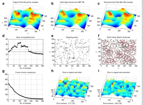
Figure 6(a-i: from left to right, then top to bottom): Simulation results for single-robot adaptive sampling.Field estimate is calculated after every sample. Norm of errorðkggestkþ1k2Þreduces to19.67 in 302 samples and it took 11.92 min.
Table 2 Comparison of computational complexity and communication overhead for centralized, decentralized, federated decentralized, and federated distributed filter
Computations Communication
Robot Fusion center Combined
Centralized filter – O(qNL3) O(qNL3) O(qN)
Completely decentralized filter O(qL3+ (N–1)rL3) – O(NqL3+N(N–1)rL3) O(N(N–1)r(L2+L))
Federated decentralized filter O(qL3) O(rL3) O(NqL3+rL3) O(2Nr(L2+L))
However, it is important to note here that, while the example here, based on a lower number (100) samples per grid, has a high initial field error, it achieves the same accuracy as the example (covered in [6]), which uses a higher number (900) of samples per grid. The ac-curacy achieved by this example is due to the fact that it relies on AS while using only a smaller total number of
samples of 100 (initial samples) + 302(adaptively
acquired) = 402 samples than the one used in the ex-ample of [6].
The other criterion is the 2-norm of the parameter error covariance matrixðkPkþ1k2Þ.
Figures 6 and 7, respectively, show the simulation results when using a single-robot sampling and a multi-robot one. It can be seen from Figure 6d that the field estimation error first increases to a peak value before it starts to decrease. This initial increase in error seems to be caused by an apparent divergence of the EKF fil-ter which is prone to divergence because of its depend-ence on the first-order linearization process that is
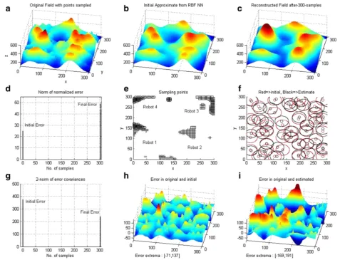
performed to calculate the new estimate. More detailed analysis of this can be found in [29] where we carried out a thorough comparison between various nonlinear filters such as the EKF, Second-order EK, Iterated EKF, and Unscented KF so as to study and highlight the lim-itations of the EKF filter. Another possible reason for this filter divergence could be the insufficient number of samples used. This can also be exacerbated by the fact that the further these few samples are apart, i.e., the larger the linearization step is, the worse the linearization error becomes. This increase in error could also be due to an insufficient coverage of the sampling area. This therefore reinforces our motivation to use multiple robots that ensure that different regions are adequately covered at the same time. The improve-ment brought about by the use of multiple robots can be seen in Figure 7d for the multi-robot case where, the initial error increase, although not completely elimi-nated, has been greatly reduced compared to the single robot case (Figure 6d).
Figure 7(a-i: from left to right, then top to bottom): Simulation results for multi-robot adaptive sampling with federated decentralized filter.Partial field estimates are calculated after every sample. Complete field estimates are calculated after every 80 samples. Norm of error
As discussed in previous sections, if the centralized fil-ter is used for multi-robots, then AS is not possible. Figure 8 shows the simulation results when all the sam-pling locations for the four robots used are generated in advance based on the initial estimate. Hence, the sampling approach is non-adaptive in nature. Robots collect samples from these locations and transmit them to the central filter for fusion. It can be clearly seen from Figure 8e that if future sampling locations gener-ated by the (non-adaptive) sampling algorithm are based on the initial estimate of error covariance only, then these locations would not provide much informa-tion about the global field distribuinforma-tion, as these loca-tions are all closer to one another and hence would furnish only a localized knowledge of the field distribu-tion. In fact, after collecting 300 samples, the error is still very high as shown in Figure 8d and Table 3. Moreover, it takes the non-negligible time of 5.48 min to perform this mission. Figure 7 shows the results for a federated decentralized approach which is equally
valid for a completely decentralized one. The only dif-ference between these two approaches will be in the computation and communication load to be carried by the robots. For the completely decentralized approach, the total number of samples collected is q= 320. After every 20 samples collected, each robot sends its partial (local) estimate to the global filter for fusion. This way this update is performedr= 4 times.
The use of four robots instead of one for sampling also reduces the time for field reconstruction from 11.92 to 2.98 min which amounts approximately to a fourfold re-duction in time. The reason for this rere-duction can be explained intuitively since, by sampling using four robots, instead of one, not only does the number of sam-ples collected by each robot gets reduced, but so does the navigation time as well because of the smaller sam-pling area allocated to each robot.
It is important to point out at this juncture that the process by which only the average number of the most influencing Gaussians is kept is based on their percent
contribution relative to the total contribution of all the Gaussians. These influencing Gaussians are selected whenever their relative percent contributions exceed a very small threshold chosen to be equal to 0.001% in our simulation.
Table 3 illustrates the number of computations and communications involved in the above simulations. For the federated distributed filter, it is assumed that on the average, each collected sample influences the estimate of
10 neighboring Gaussians, and each communication up-date transmits the estimates of 15 Gaussians. Hence, the average number of parameters that can change after each sample is M= 41, since there are 10 Gaussians, 4 parameters per Gaussian and 1 free offset parameter (i.e.,
M¼4Bþ1¼410þ1 ).Furthermore in our
simula-tion we are assuming that the number of all the para-meters expected to change is equal to the number of all
the parameters that actually change, i.e., S¼C¼
Table 3 Comparison of computational loads and communication overheads for centralized, completely
decentralized, federated decentralized and federated distributed filters for sampling of the complex field shown in Figures 6, 7, and 8
Computations Communication
Robot Fusion Center Combined
Centralized filter – 1.34 × 10⁶ 1.34 × 10⁶ 320
Completely decentralized filter 383.94 × 10⁶ – 1,535.77 × 106 1,251.94 × 103
Federated decentralized filter 333.86 × 10⁶ 16.69 × 10⁶ 1,352.13 × 106 834.62 × 10³
Federated distributed filter 5.51 × 10⁶ 16.69 × 10⁶ 38.73 × 10⁶ 121.02 × 10³
4Bþ1¼415þ1 . Using the formulae shown in Table 2 to calculate the number of computations and communication, the results we get for the federated decentralized case are, respectively, 1.14 and 1.5 times smaller than their counterparts in the completely decen-tralized case. Moreover, the number of computations and communication in the federated distributed case are, re-spectively, 35 and 7 times smaller than their counterparts in the federated decentralized case.
Scalability
The scalability of the proposed federated distributed al-gorithm is discussed here by comparing the numbers of computations and packets communicated (i.e., the com-putational and communication load) in two different scenarios, as explained below.
i. The number of sampling robots increases but the number of field parameters is kept unchanged. As the number of sampling robots increases, the computational and communication load increases almost linearly in the case of both the federated decentralized and distributed filters, whereas for the completely decentralized filter, this load increases quadratically. Figures9and10, respectively, show that the computational and communication loads increase when the number of robots used increases from 4 to 20 for all 4 types of filter structures. ii. The number of parameters representing the field
increases but the number of robots remains
unchanged. This scenario may represent different cases where either a highly complex field is used which requires a large number of parameters for its description but does not necessarily cover a wide area or a field that is modestly complex but ranges over a very wide area or possibly a field that combines both features. If the field is spread over a wide area, and the number of robot is kept unchanged, then it would require more time to reconstruct the field and the number of
computations and communications would depends on the number of parameters used to represent the field.
Figures11and12, respectively, show the
computational and communicational loads when the increasing numbers of parameters used are 161, 241, 321, 401, and 481. These five scenarios reflect the cases where the field is represented with 40, 60, 80, 100, and 120 Gaussians, respectively. As shown in Table2, the computational complexity is related cubically to the number of parameters. But, in the case of the distributed KF algorithm, the rate of increase is far smaller than the one for the other three filters as shown in Figure11. This result is expected since, for the distributed KF filter, the complexity is proportional toM3rather than toL3, andM<L. The computational complexity can be further reduced by increasing the number of robots as the number of parameters increases as this will reduce the factorM.
4 8 12 16 20
Number of computations versus number of sampling robots
4 8 12 16 20
The communication complexity is related quadratically to the number of parameters for the completely decentralized and federated decentralized filters. For the centralized filter, this complexity is not a function of the number of parameters, because it is the measurementZ,rather than the parameter estimate, that is transmitted. For the federated distributed filter, the communication complexity is
related quadratically to the number of parameters. However, when the number of parameters increases, the rate of growth of the communication load is smaller is smaller than the corresponding rate for the completely decentralized and federated decentralized filters. The reason for this is that it is
Mand C, rather than the largerL, that are, respectively, used in the last two entries in the
2 4 6 8 10 12 14 16 18 20 22
s Number of communications versus number of sampling robots
4 8 12 16 20
Figure 11Number of computations versus number of field parameters when number of sampling robots remains unchanged.
161 241 321 401 481
0 2 4 6x 10
11
Number of field parameters
N
Number of computations versus number of field parameters
161 241 321 401 481
0 5 10x 10
9
Number of field parameters
N
Number of communications versus number of field parameters centralized filter
completely decentralized filter federated decentralized filter
federated distributed filter
columns titled:“Combined”and“Communications” in Table2.
Conclusion
In this article, we studied the problem of estimating the field distribution of some particular environmental vari-able (e.g., moisture, salinity, etc.) using both single-robot and multi-robot AS schemes and different filtering structures, such as the centralized and decentralized ones as well as our proposed federated distributed filter-ing structure. Our thorough simulation study,
encom-passing various AS schemes, clearly showed the
superiority of using multi-robot-based AS schemes over their single-robot-AS counterparts.
These attractive advantages enjoyed by the multi-robot AS schemes are mainly due to their features of parallel sampling, a wider area coverage and a decentralization scheme offered by the multi-robot approach. We pro-posed a novel scalable structure termed the decentra-lized distributed filter approach where the full-order local KF filter used in the conventional decentralized ap-proach has been distributed into several low-order KFs, thus leading to a further vital reduction in the field re-construction time. Our simulation results corroborated very well our expectations of the higher performance of our novel decentralization-cum-distribution approach since the estimates of the communication and computa-tional loads on the Nrobots used show that a dramatic in-excess of-N-fold reduction in the sampling time can be achieved, leading to a similar reduction in the field reconstruction time. These very encouraging results pro-vide us with ample encouragement to further investigate both the efficiency and convergence properties of our proposed distributed filter scheme. This analytical inves-tigation as well as our ultimate goal of successfully test-ing our proposed approach on a physical multi-robot system is both currently under way.
Competing interests
The authors declare that they have no competing interests.
Acknowledgment
This study was supported by the King Fahd University of Petroleum and Minerals, Dhahran, Saudi Arabia, Projects # JF090014 and SB101017.
Author details
1Systems Engineering Department, King Fahd University of Petroleum and
Minerals, Dhahran 31261, Saudi Arabia.2Electrical Engineering Department,
The University of Texas at Arlington, Arlington, TX 76019, USA.
Received: 21 July 2011 Accepted: 30 May 2012 Published: 18 July 2012
References
1. W. Jatmiko, K. Sekiyama, T. Fukuda, A mobile robots PSO-based for odor source localization in dynamic advection–diffusion environment, inIEEE/RSJ International Conference on Intelligent Robots and Systems(2006), pp. 4527–4532
2. V.N. Christopoulos, S. Roumeliotis, Adaptive sensing for instantaneous gas release parameter estimation, inIEEE International Conference on Robotics and Automation(2005), pp. 4450–4456
3. D.A. Robinson, C.S. Campbell, J.W. Hopmans, B.K. Hornbuckle, S.B. Jones, R.O. Knight, F. Ogden, J. Selker, O. Wendroth, Soil moisture measurement for ecological and hydrological watershed-scale observatories: a review. Vadose Zone J.7, 358–389 (2008)
4. C.J. Cannell, D.J. Stilwell, A comparison of two approaches for adaptive sampling of environmental processes using autonomous underwater vehicles, inProceedings of MTS/IEEE OCEANS(2005), pp. 1514–1521 5. N.E. Leonard, D. Paley, F. Lekien, R. Sepulchre, D.M. Fratantoni, R. Davis,
Collective motion, sensor networks and ocean sampling. Proc. IEEE95(1), 48–74 (2007)
6. M.F. Mysorewala, D.O. Popa, Multi-scale adaptive sampling with mobile agents for mapping of forest fires. J. Intell. Robot. Syst.54(4), 535–565 (2009) 7. V. Hombal, A.C. Sanderson, R. Blidberg, A non-parametric iterative algorithm
for adaptive sampling and robotic vehicle path planning, inIEEE/RSJ International Conference on Intelligent Robots and Systems(2006), pp. 217–222
8. A. Singh, A. Krause, C. Guestrin, W. Kaiser, Efficient informative sensing using multiple robots. J. Artif. Intell. Res. (JAIR)34, 707–755 (2009)
9. M.A. Demetriou, I.I. Hussein, Estimation of spatially distributed processes using mobile spatially distributed sensor network. SIAM J. Control. Optim. 48, 266–291 (2009)
10. S. Martinez, Distributed interpolation schemes for field estimation by mobile sensor networks. IEEE Trans. Control. Syst. Technol.18(2), 491–500 (2010) 11. NAC Cressie,Statistics for Spatial Data, Revisedth edn. (Wiley, New York,
1993)
12. M.L. Stein,Interpolation of Spatial Data. Some Theory for Kriging. Springer Series in Statistics(Springer, New York, 1999)
13. J. Cortes, Distributed Kriged Kalman filter for spatial estimation. IEEE Trans. Automat. Control54(12), 2816–2827 (2009)
14. R. Graham, J. Cortes, Spatial statistics and distributed estimation by robotic sensor networks, inAmerican Control Conference (ACC)(2010),
pp. 2422–2427
15. R. Graham, J. Cortes, Cooperative adaptive sampling of random fields with partially known covariance. Int. J. Robust Nonlinear Control22(5), 504–534 (2012)
16. R. Olfati-Saber, Distributed Kalman filter with embedded consensus filters, in 44th IEEE Conference on Decision and Control, 2005 and 2005 European Control Conference. CDC-ECC '05(2005), pp. 8179–8184
17. R. Olfati-Saber, Distributed Kalman filtering for sensor networks, in46th IEEE Conference on Decision and. Control2007(12–14), 5492–5498 (2007) 18. A. Singh, D. Budzik, W. Chen, M. Batalin, M. Stealey, H. Borgstrom, W. Kaiser,
Multiscale sensing: a new paradigm for actuated sensing of high frequency dynamic phenomena, inIEEE/RSJ International Conference on Intelligent Robots and Systems, 2006(2006), pp. 328–335
19. A.G. Mutambara,Decentralized Estimation and Control for Multisensor Systems, Chapters 2–3(CRC Press, Boca Raton, 1998), pp. 19–79. doi:19 20. H.R. Hashmipour, S. Roy, A.J. Laub, Decentralized structures for parallel
Kalman filtering. IEEE Trans. Automat. Control33(1), 88–93 (1988) 21. Y. Gao, E.Y. Krakiwsky, M.A. Abousalem, J.F. Mclellan, Comparison and
analysis of centralized, decentralized, and federated filters. Navigation40(1), 69–86 (1993)
22. M.F. Mysorewala, L. Cheded, M.S. Baig, D.O. Popa, A distributed multi-robot adaptive sampling scheme for complex field estimation, in11th International Conference on Control Automation Robotics & Vision (ICARCV) 2010, 7–10(2010), pp. 2466–2471
23. D.O. Popa, M.F. Mysorewala, F.L. Lewis, EKF-based adaptive sampling with mobile robotic sensor nodes, inInternational Conference on Intelligent Robots and Systems, 2006 IEEE/RSJ(2006), pp. 2451–2456
24. Q. Du, V. Faber, M. Gunzburger, Centroidal voronoi tessellations: applications and algorithms. SIAM Rev.41, 637–676 (1999)
25. J.C. Bezdek,Pattern Recognition with Fuzzy Objective Function Algorithms( Kluwer Academic Publishers(Norwell, MA, 1981)
26. B.S. Rao, H.F. Durrant-Whyte, Fully decentralized algorithm for multisensor Kalman filtering. IEE Proc. Control Theory Appl.138, 413–420 (1991) 27. N.A. Carlson, Federated square root filter for decentralized parallel processes.
IEEE Trans. Aerospace Electron. Syst.26(3), 517–525 (1990)
underwater vehicles, inAutonomous Underwater Vehicles(2004), pp. 108–118
29. M.F. Mysorewala, L. Cheded, A. Qureshi, Comparison of nonlinear filters for the estimation of parametrized spatial field by robotic sampling, in6thIEEE conference on Industrial Electronics and Applications(2011), pp. 2005–2010 30. S. Haykin,Neural Networks: A Comprehensive Foundation, Secondth edn.
(Prentice Hall PTR, 1998)
doi:10.1186/1687-1499-2012-223
Cite this article as:Mysorewalaet al.:A distributed multi-robot adaptive sampling scheme for the estimation of the spatial distribution in widespread fields.EURASIP Journal on Wireless Communications and
Networking20122012:223.
Submit your manuscript to a
journal and benefi t from:
7Convenient online submission
7Rigorous peer review
7Immediate publication on acceptance
7Open access: articles freely available online
7High visibility within the fi eld
7Retaining the copyright to your article