A New Class of Particle Filters for Random Dynamic
Systems with Unknown Statistics
Joaqu´ın M´ıguez
Departamento de Electr´onica e Sistemas, Universidade da Coru˜na, Facultade de Inform´atica, Campus de Elvi˜na s/n, 15071 A Coru˜na, Spain
Email:[email protected]
M ´onica F. Bugallo
Department of Electrical and Computer Engineering, State University of New York at Stony Brook, Stony Brook, NY 11794-2350, USA
Email:[email protected]
Petar M. Djuri´c
Department of Electrical and Computer Engineering, State University of New York at Stony Brook, Stony Brook, NY 11794-2350, USA
Email:[email protected]
Received 4 May 2003; Revised 29 January 2004
In recent years, particle filtering has become a powerful tool for tracking signals and time-varying parameters of random dynamic systems. These methods require a mathematical representation of the dynamics of the system evolution, together with assumptions of probabilistic models. In this paper, we present a new class of particle filtering methods that do not assume explicit mathematical forms of the probability distributions of the noise in the system. As a consequence, the proposed techniques are simpler, more robust, and more flexible than standard particle filters. Apart from the theoretical development of specific methods in the new class, we provide computer simulation results that demonstrate the performance of the algorithms in the problem of autonomous positioning of a vehicle in a 2-dimensional space.
Keywords and phrases:particle filtering, dynamic systems, online estimation, stochastic optimization.
1. INTRODUCTION
Many problems in signal processing can be stated in terms of the estimation of an unobserved discrete-time random signal in a dynamic system of the form
xt= fx(xt−1) +ut, t=1, 2,. . ., (1) yt= fy(xt) +vt, t=1, 2,. . ., (2)
where
(a) xt ∈RLxis the signal of interest, which represents the system state at timet;
(b) fx : RLx → Ix ⊆ RLx is a (possibly nonlinear) state
transition function;
(c) ut ∈ RLx is the state perturbation or system noise at
timet;
(d) yt∈RLyis the vector of observations collected at time t, which depends on the system state;
(e) fy:RLx→Iy⊆RLy is a (possibly nonlinear)
transfor-mation of the state;
(f) vt ∈RLy is the observation noise vector at timet, as-sumed statistically independent from the system noise ut.
Equation (1) describes the dynamics of the system state vec-tor and, hence, it is usually termedstate equationorsystem equation, whereas (2) is commonly referred to asobservation equation or measurement equation. It is convenient to dis-tinguish the structure of the dynamic system defined by the functions fxand fyfrom the associated probabilistic model, which depends on the probability distribution of the noise signals and the a priori distribution of the state, that is, the statistics ofx0.
of the state at timetis contained in the so-calledfiltering pdf, that is, the a posteriori density of the system state given the observations up to timet,
pxt|y1:t
, (3)
where y1:t = {y1,. . .,yt}. The density (3) usually involves a multidimensional integral which does not have a closed-form solution for an arbitrary choice of the system structure and the probabilistic model. Indeed, analytical solutions can only be obtained for particular setups. The most classical ex-ample occurs when fx and fy are linear functions and the noise processes are Gaussian with known parameters. Then the filtering pdf of xt is itself Gaussian, with meanmt and covariance matrixCt, which we denote as
pxt|y1:t
=Nmt,Ct
, (4)
where the posterior parameters mt and Ct can be recur-sively computed, as time evolves, using the elegant algorithm known as Kalman filter (KF) [1]. Unfortunately, the assump-tions of linearity and Gaussianity do not hold for most real-world problems. Although modified Kalman-like solu-tions that account for general nonlinear and non-Gaussian settings have been proposed, including the extended KF (EKF) [2] and the unscented KF (UKF) [3], such tech-niques are based on simplifications of the system dynam-ics and suffer from severe degradation when the true dy-namic system departs from the linear and Gaussian assump-tions.
Since general analytical solutions are intractable, Baye-sian estimation in nonlinear, non-GausBaye-sian systems must be addressed using numerical techniques. Deterministic ap-proaches, such as classical numerical integration procedures, turn out ineffective or too demanding except for very low-dimensional systems and, as a consequence, methods based on the Monte Carlo methodology have progressively gained momentum. Monte Carlo methods are simulation-based techniques aimed at estimating the a posteriori pdf of the state signal given the available observations. The pdf esti-mate consists of a random grid of weighted points in the state spaceRLx. These points, usually termedparticles, are Monte
Carlo samples of the system state that are assigned nonnega-tiveweights, which can be interpreted as probabilities of the particles.
The collection of particles and their weights yield an em-pirical measure which approximates the continuous a poste-riori pdf of the system state [4]. The recursive update of this measure whenever a new observation is available is known as particle filtering (PF). Although there are other popular Monte Carlo methods based on the idea of producing em-pirical measures with random support, for example, Markov Chain Monte Carlo (MCMC) techniques [5], PF algorithms have recently received a lot of attention because they are par-ticularly suitable for real-time estimation. The sequential im-portance sampling (SIS) algorithm [6,7] and the bootstrap filter (BF) [8,9] are the most successful members of the PF class of methods [10]. Existing PF techniques rely on
(i) the knowledge of the probabilistic model of the dy-namic system (1)-(2), which includes the densities p(x0),p(ut), andp(vt),
(ii) the ability to numerically evaluate the likelihood p(yt|xt) and to sample from the transition density p(xt|xt−1).
Therefore, the practical performance of PF algorithms in real-world problems heavily depends on how accurate the underlying probabilistic model of choice is. Although this may seem irrelevant in engineering problems where it is rel-atively straightforward to associate the observed signals with realistic and convenient probability distributions, in many situations, this is not the case. Many times, it is very hard to find an adequate model using the information available in practice. In other occasions, the working models obtained after a lot of effort (involving, e.g., time-series analysis tech-niques) are so complicated that they render any subsequent signal processing algorithm impractical due to its high com-plexity.
In this paper, we introduce a new PF approach to deal with uncertainty in the probabilistic modeling of the dy-namic system (1)-(2). We start with the requirement that the ultimate objective of PF is to yield an estimate of the sig-nals of interest x0:t, given the observationsy1:t. If a suitable probabilistic model is at hand, good signal estimates can be computed from the filtering pdf (3) induced by the model, and a PF algorithm can be employed to recursively build up a random grid that approximates the posterior distribution. However, it is often possible to use signal estimation methods that do not explicitly rely on the a posteriori pdf, for example, blind detection in digital communications can be performed according to several criteria, such as the constrained mini-mization of the received signal power [11] or the constant modulus method [12,13]. Such approaches are very popular because they are based on a simple figure of merit, and this simplicity leads to robust and easy-to-design algorithms.
As long as a recursive decomposition of the cost function is found, a PF algorithm, similar to the SIS and bootstrap meth-ods, can be used to construct a random-grid approximation of the cost function in the vicinity of its minima. For this rea-son, CRPFs yield localrepresentations of the cost function specifically built to facilitate the computation of minimum-cost estimates of the state signal.
The remainder of this paper is organized as follows. The fundamentals of the CRPF family are introduced in Section 2. This includes three basic building blocks: thecost andriskfunctions, which provide a measure of the quality of the particles, and the stochastic mechanism for particle gen-eration and sequential update of the random grid. Since the usual tools for PF algorithm design (e.g., proposal distribu-tions, auxiliary variables, etc.) do not necessarily extend to the new framework, this section also contains a discussion on design issues. In particular, we identify the factors on which the choice of the cost and risk functions will usually depend, and derive consequent design guidelines, including a useful choice of parameters that leads to a simple interpretation of the algorithm and its connection with the theory of stochas-tic approximation (SA) [14].
Due to the change in the reference, convergence results regarding SRPFs are not valid for CRPFs.Section 3is devoted to the problem of identifying sufficient conditions for asymp-totically optimal propagation(AOP) of particles. The stochas-tic procedure for drawing new samples of the state signal and propagating the existing particles using the new samples is the key for the convergence of the algorithm. We term this particle propagation step as asymptotically optimal when the increment in the average cost of the particles in the filter after propagation is minimal. A set of sufficient conditions for op-timal propagation, related to the properties of the sampling and weighting methods, is provided.
Section 4is devoted to the discussion ofresamplingin the new family of PF techniques. We argue that the objective of this important algorithmic step is different from its usual role in conventional PF algorithms, and exploit this difference to propose alocal resamplingscheme suitable for a straight-forward implementation using parallel VLSI hardware (note that resampling is a major bottleneck for the parallel imple-mentation of PF methods [15]).
Computer simulation results that illustrate the validity of our approach are presented inSection 5. In particular, we tackle the problem of positioning a vehicle that moves along a 2-dimensional space. An instance of the proposed CRPF class of methods that employs a simple cost function is com-pared with the standard auxiliary BF [9] technique. Finally, Section 6contains conclusions.
2. COST-REFERENCE PARTICLE FILTERING
The basics of the new family of PF methods are introduced in this section. We start with a general description of the CRPF technique, where key concepts, namely, the cost and risk functions, particle propagation, and particle selection, are introduced. The second part of the section is devoted to practical design issues. We suggest guidelines for the design
of CRPFs and propose a simple choice of the algorithm pa-rameters that lead to a straightforward interpretation of the CRPF technique.
2.1. Sequential algorithm
The ultimate aim of the method is the online estimation of the sequence of system states from the available observations, that is, we intend to estimatext|y1:t,t =0, 1, 2,. . ., accord-ing to some reference function that yields a quantitative mea-sure of quality. In particular, we propose the use of a realcost function with a recursive additive structure, that is,
Cx0:t|y1:t,λ
=λCx0:t−1|y1:t−1,λ
+Cxt|yt
, (5)
where 0< λ <1 is a forgetting factor,C :RLx×RLy →R
is theincremental costfunction, andC(x0:t|y1:t,λ) complies with the definition
C:R(t+1)Lx×RtLy×R−→R. (6)
We should remark that (5) is not the only recursive decom-position that can be employed. A straightforward alternative is to choose a cost function which is built at timet as the convex sum
Cx0:t|y1:t,λ
=λCx0:t−1|y1:t−1,λ
+ (1−λ)C(xt|yt). (7)
This form of cost function is perfectly valid for the defini-tion and construcdefini-tion of CRPFs and choosing it would not affect (or would affect trivially) the arguments presented in the rest of this paper, including the asymptotic convergence results inSection 3. However, we will constrain ourselves to the familiar form of (5) for simplicity.
A high value of C(x0:t|y1:t,λ) means that the state se-quencex0:tis not a good estimate given the sequence of ob-servations y1:t, while a low value ofC(x0:t|y1:t,λ) indicates thatx0:t is close to the true state signal. The sequencex0:tis said to have a high cost, in the former case, or a low cost, in the latter case. Particularly notice the recursive structure in (5), where the cost of a sequence up to timet−1 can be up-dated by solely looking at the state and observation vectors at timet,xt, andyt, respectively, which are used to compute the cost incrementC(xt|yt). The forgetting factorλavoids attributing an excessive weight to old observations when a long series of data are collected, hence allowing for potential adaptivity.
We also introduce a one-stepriskfunction of the form
R:RLx×RLy −→R, xt−1,ytR
xt−1|yt
(8)
that measures the adequacy of the state at timet−1 given the new observationyt. It is convenient to view the risk function
R(xt−1|yt) as a prediction of the cost incrementC(xt|yt) that can be obtained beforextis actually propagated. Hence, a natural choice of the risk function is
Rxt−1yt
= Cfxxt−1yt
The proposed estimation technique proceeds sequen-tially in a similar manner as the BF. Given a set of M state samples and associated costs up to time t, that is, the weighted-particle set (wps)
Ξt=
x(ti),Ct(i) M
i=1, (10)
where Ct(i) = C(x0:(i)t|y1:t,λ), the grid of state trajectories is randomly propagated whenyt+1is observed in order to build
an updated wpsΞt+1. The state and observation signals are
those described in the dynamic system (1)-(2). We only add the following mild assumptions:
(1) the initial state is known to lie in a bounded interval Ix0⊂RLx;
(2) the system and observation noise are both zero mean.
Assumption (1) is needed to ensure that we initially draw a set of samples that is not infinitely far from the true statex0.
Notice that this is a structural assumption, not a probabilis-tic one. Assumption (2) is made for the sake of simplicity because zero-mean noise is the rule in most systems.
The sequential CRPF algorithm based on the structure of system (1)-(2), the definitions of cost and risk functions given by (5) and (8), respectively, and assumptions (1) and (2), is described below.
(1)Timet=0(initialization).DrawMparticles from the uniform distribution in the intervalIx0,
x(0i)∼U
Ix0
, (11)
and assign them a zero cost. The initial wps
Ξ0=
x(0i),C(0i)=0
M
i=1 (12)
is obtained.
(2)Timet+ 1(selection of the most promising trajectories). The goal of the selection step is to replicate those particles with a low cost while high-cost particles are discarded. As usual in PF methods, selection is implemented by a resam-pling procedure [7]. We point out that, differently from the standard BF, resampling in CRPFs does not produce equally weighted particles. Instead, each particle preserves its own cost. Notice that the equal weighting of resampled particles in standard PF algorithms comes from the use of a statisti-cal reference. In CRPF, preserving the particle costs after re-sampling actually shifts the random grid representation of the cost function toward its local minima. Such a behavior is sound, as we are interested in minimum cost signal esti-mates. Further issues related to resampling are discussed in Section 4.
Fori=1, 2,. . .,M, compute the one-step risk of particle iand let
R(i)
t+1=λC (i)
t +R
x(ti)|yt+1
(13)
which yields a predictive cost of the trajectoryx0:taccording to the new observationyt. Define a probability mass function (pmf) of the form
ˆ πt(+1i) ∝µ
R(i)
t+1
, (14)
whereµ:R →[0, +∞) is a monotonically decreasing func-tion. An intermediate wps is obtained by resampling the trajectories{x(ti)}Mi=1 according to the pmf ˆπ
(i)
t+1. Specifically,
we select ˆx(ti) = xt(k) with probability ˆπt(+1k), and build the
set ˆΞt+1 = {xˆt(i), ˆCt(i)}Mi=1, where ˆCt(i) = Ct(k) if and only if ˆ
x(ti)=x(tk).
(3)Time t+ 1(random particle propagation).Select an arbitrary conditional pdf of the state pt+1(xt+1|xt) with the constraint that
Ept+1(xt+1|xt)
xt+1
= fxxt
, (15)
whereEp(s)[·] denotes expected value with respect to the pdf
in the subindex. Using the selected propagation density, draw new particles
x(ti+1) ∼pt+1
xt+1|xˆ(ti)
(16)
and update the associated costs
C(i)
t+1=λCˆ (i)
t +Ct(+1i), (17)
where
C(i)
t+1= C
x(t+1i)yt+1
(18)
fori=1, 2,. . .,M.
As a result, the updated wpsΞt+1 = {x(t+1i),Ct(+1}i) Mi=1is
ob-tained.
(4)Timet+ 1(estimation of the state).Estimation pro-cedures are better understood if a pmfπt(+1i),i=1, 2,. . .,M,
is assigned to the particles inΞt+1. The natural way to define
this pmf is according to the particle costs, that is,
πt(+1i) ∝µ
C(i)
t+1
, (19)
whereµis a monotonically decreasing function.
The minimum cost estimate at timet+ 1 is trivially com-puted as
i0=arg max
i
πt(+1i)
,
˜ xmin0:t+1=x
(i0) t+1
and its physical meaning is obvious. An equally useful esti-mate can be computed as the mean value ofx(ti+1) according to the pmfπt(+1i), that is,
˜ xmean
t+1 =
M
i=1
πt(+1i)x (i)
t+1. (21)
Note that ˜xmeant+1 can also be regarded as a minimum cost
es-timate because the particle set Ξt+1 is a random-grid local
representation of the cost function in the vicinity of its min-ima. In fact, estimator (21) has slight advantages over (20). Namely, the averaging of particles according to the pmfπt(+1i)
yields an estimated state trajectory which is smoother than the one resulting from simply choosing the particle with the least cost at each time step. Besides, computing the mean of the particles underπt(+1i) may result in an estimate with a
slightly smaller cost than the least cost particle, since ˜xtmean+1
is obtained by interpolation of particles around the least cost state.
Sufficient conditions for the mean estimate (21) to attain an asymptotically minimum cost are given inSection 3.
We will refer to the general procedure described above as a CRPF algorithm. It is apparent that many implementations are possible for a single problem, so in the next section, we discuss the choice of the functions and parameters involved in the method.
2.2. Design issues
An instance of the CRPF class of algorithms is selected by choosing
(i) the cost functionC(·|·), (ii) the risk functionR(·|·),
(iii) the monotonically decreasing functionµ : R → [0, +∞) that maps costs and risks into the resampling and estimation pmfs, as indicated in (14) and (19), respec-tively,
(iv) the sequence of pdfspt+1(xt+1|xt) for particle genera-tion.
The cost and risk functions measure the quality of the par-ticles in the filter. Recall that the risk is conveniently inter-preted as a prediction of the cost of a particle, given a new ob-servation, before random propagation is actually carried out (see the selection step inSection 2.1). Therefore, the cost and the risk should be closely related, and we suggest to choose
R(·|·) according to (9). Whenever possible, both the cost and risk functions should be
(i) strictly convex in the range of values ofxt, where the state is expected to lie, in order to avoid ambiguities in the estimators (20) and (21) as well as in the selection (resampling) step,
(ii) easy to compute in order to facilitate the practical im-plementation of the algorithm,
(iii) dependent on the complete state and observation sig-nals, that is, it should involve all the elements ofxtand yt.
A simple, yet useful and physically meaningful, choice of
C(·|·,·),R(·|·) that will be used in the numerical examples ofSection 5is given by
Cx0
=0, (22)
Cxtyt
= yt−fy
xt q, (23)
Rxtyt+1
= yt+1−fy
fxxt q, (24)
whereq≥1 andv =√vTvdenotes the norm ofv. Given a
fixed and bounded sequence of observationsy1:t, the optimal (minimum cost) sequence of state vectors is
xopt0:t =arg minx 0:t
Cx0:ty1:t,λ
=arg min
x0:t t
k=0
λ(t−k)Cx
tyt
.
(25)
We callxopt0:t optimal because it is obtained by minimization of the continuous cost function, and it is in general different from the minimum cost estimate obtained by CRPF, which we have denoted as ˜x0:mint inSection 2.1.
With the assumed choice of cost and risk functions given by (22)–(24), the invertible observation functionfy:RLx →
Iy ⊆RLy,andyt ∈Iy, for allt≥1, it is straightforward to
derive a pointwise solution of the form1
xoptt =arg min
xt
Cxtyt
= f−1
y
yt
. (26)
Therefore, as the CRPF algorithm randomly selects and propagates the sample states with the least cost, it can be un-derstood (again, under assumption of (22)–(24)) as a nu-merical stochastic method for approximately solving the set of (possibly nonlinear) equations
yt−fy
xt
=0, t=1, 2,. . . . (27)
Furthermore, setting q = 1 in (23) and (24), we obtain a Monte Carlo estimate of the mean absolute deviation solu-tion of the above set of equasolu-tions, whileq = 2 results in a stochastic optimization of the least squares type.
This interpretation of the CRPF algorithm as a method for numerically solving (27) allows to establish a connec-tion between the proposed methodology and the theory of SA [14], which is briefly commented upon inAppendix A.
The function µ : R → [0, +∞) should be selected to guarantee an adequate discrimination of low-cost particles from those presenting higher costs (recall that we are inter-ested in computing a local representation of the cost func-tion in the vicinity of its minima). As shown in Section 5, the choice ofµhas a direct impact on the algorithm perfor-mance. Specifically, notice that the accuracy of the selection step is highly dependent on the ability of µto assign large probability masses to lower-cost particles.
A straightforward choice of this function is
µ1
C(i)
t
=C(i)
t −1
, Ct(i)∈R\ {0}, (28)
which is simple to compute and potentially useful in many systems. It has a serious drawback, however, in situations where the range of the costs, that is, maxi{C(i)
t }−mini{Ct(i)}, is much smaller than the average cost (1/M)Mi=1Ct(i). In such scenarios,µ1 yields nearly uniform probability masses
and the algorithm performance degrades. Better discrimina-tion properties can be achieved with an adequate modifica-tion ofµ1, for example, with
µ2
C(i)
t
= 1
C(i)
t −mink
C(k)
t
+δβ, (29)
where 0 < δ < 1 andβ > 1. When compared withµ1,µ2
assigns larger masses to low-cost particles and much smaller masses to higher-cost samples. The discrimination ability of µ2is enhanced by reducing the value ofδ(i.e.,δ0) and/or
increasingβ. The relative merit ofµ2overµ1 is
experimen-tally illustrated inSection 5.
The last selection to be made is the pdf for particle prop-agation, pt+1(xt+1|xt), in step 3 of the CRPF algorithm. The theoretical properties required for optimalpropagation are explored inSection 3. From a practical and intuitive2point
of view, it is desirable to use easy-to-sample pdfs with a large enough variance to avoid losing tracks of the state signal, but not too large, to prevent the generation of too dispersed particles. A simple strategy implemented in the simulations ofSection 5consists of using zero-mean Gaussian densities with adaptively selected variance. Specifically, the particleiis propagated from timetto timet+ 1 as
x(ti+1) ∼N
fxxˆ(t−i)1
,σt2,(i)ILx
, (30)
whereILx is theLx×Lx identity function and the variance
σt2,(i)is recursively computed as
σt2,(i)=t− 1 t σ
2,(i)
t−1 +
x(i)
t −fx
ˆ x(t−i)1
2
tLx . (31)
This adaptive-variance technique has appeared useful and ef-ficient in our simulations, as illustrated inSection 5, but al-ternative approaches (including the simple choice of a fixed variance) can also be successfully exploited.
3. CONVERGENCE OF CRPF ALGORITHMS
In this section, we assess the convergence of the proposed CRPF algorithm. In particular, we seek sufficient conditions
2Part of this intuition is confirmed by the convergence theorem in Section 3.
for AOP of the particles from time t−1 to time t. Let Ξt = {x(ti),Ct(i)}Mi=1 be the wps computed at timet. We say
thatΞthas been obtained by AOP fromΞt−1if and only if
lim M→∞C
xoptt yt
− Ct=0 (in some sense), (32)
wherexoptt is the optimal state according to (26) and
Ct=
M
i=1
(ti)Ct(i), (33)
with a pmft(i)∝µ(Ct(i)), is the mean incremental cost at timet. The results presented in this section prove that AOP can be ensured by adequately choosing the propagation den-sity and functionµ:R→[0,∞) that relates the cost to the pmf ’s ˆπt(i)andπt(i). Notice thatπt(i)=t(i)whenλ=0.
A corollary of the AOP convergence theorem is also es-tablished that provides sufficient conditions for the mean state estimate given by (21), for the caseλ=0, to be asymp-totically optimal in terms of its incremental cost.
3.1. Preliminary definitions
Some preliminary definitions are necessary before stating and proving sufficient AOP conditions. If the selection and propagation steps of the CRPF method are considered jointly, it turns out that, at timet,Mparticles are sampled as
x(ti)∼pMt (x), (34)
whereM <∞denotes the number of particles available at timet−1 and sampling the pdfpM
t (x) amounts to resam-plingMtimes inΞt−1 = {xt−(i)1,C
(i)
t−1}M
i=1and then
propagat-ing the resultpropagat-ing particles and updatpropagat-ing the costs to build the new wps Ξt = {x(ti),Ct(i)}Mi=1 (note that we explicitly allow
M =M). Although other possibilities exist, for example, as described inSection 4, when multinomial resampling is used in the selection step of the CRPF algorithm, the pdf in (34) is a finite mixture of the form
pMt (x)= M
k=1
ˆ πt(k)pt
xx(t−k)1
. (35)
We also introduce the following notation for a ball cen-tered atxoptt with radiusε >0:
Sxoptt ,ε=x∈RLx: x−xopt
t < ε
, (36)
and we write
SMxopt t ,ε
=x∈x(ti)i=M1: x−xoptt < ε (37)
3.2. Convergence theorem
Lemma 1. Let{x(ti)}Mi=1be a set of particles drawn at time t
using the propagation pdfpM
t (x)as defined by(34), lety1:tbe a fixed bounded sequence of observations, and letC(x|yt)≥0 be a continuous cost function, bounded in S{xoptt ,ε}, with a minimum atx=xtopt.
Ifthe three following conditions are met:
(1) any ball with center atxoptt has a nonzero probability un-der the propagation density, that is,
S{xoptt ,ε}
pM
t (x)dx=γ >0 ∀ε >0, (38)
(2) the supremum of the function µ(C(·|·)) for points outsideS(xoptt ,ε)is a finite constant, that is,
Sout= sup xt∈RLx\S(xoptt ,ε)
µCxtyt
<∞, (39)
(3) the supremum of the functionµ(C(·|·))for points in-sideSM(xopt
t ,ε)converges to infinity faster than the iden-tity function, that is,
lim M→∞
M
Sin =0, (40)
where
Sin= sup xt∈SM(xoptt ,ε)
µCxtyt
, (41)
then the set functionµt:A⊆ {xt(i)}M
i=1→[0,∞)defined as
µtA⊆xt(i)Mi=1= x∈A
µCxyt
(42)
is an infinite discrete measure (see definition in, e.g., [16]) that satisfies
lim M→∞Pr
1−µt
SMxopt
t ,ε
µtx(ti)Mi=1 ≥δ
=0 ∀δ >0, (43)
wherePr[·]denotes probability, that is,
lim M→∞
µtSMxopt t ,ε
µtx(ti) M
i=1
=1 (i.p.), (44)
where i.p. stands for “in probability.”
SeeAppendix Bfor a proof.
Theorem 1. If conditions (38), (39), and (40) inLemma 1 hold true, then the mean incremental cost at timet,
Ct=
M
i=1
(ti)C
x(ti)yt
, (45)
converges to the minimal incremental cost asM→ ∞,
lim M→∞C
xtoptyt
− Ct=0 (i.p.). (46)
SeeAppendix Cfor a proof.
Finally, an interesting corollary that justifies the use of the mean estimate (21) can be easily derived fromLemma 1and Theorem 1.
Corollary 1. Assuming(38),(39), and(40)inLemma 1, and forgetting factorλ=0, the mean cost estimate is asymptotically optimal, that is,
lim M→∞C
˜ xmean
t yt
− Ct
xoptt |yt=0 (i.p.), (47)
where
˜ xmean
t =
M
i=1
πt(i)xt(i). (48)
SeeAppendix Dfor a proof.
3.3. Discussion
Theorem 1states that conditions (38)–(40) are sufficient to achieve AOP (i.p.). The validity of this result clearly depends on the existence of a propagation pdf,pM
t [·], and a measure µtwithgoodproperties in order to meet the required condi-tions.
It is impossible to guarantee that condition (38) holds true in general, as the value ofxtoptis a priori unknown, but if the number of particles is large enough and they are evenly distributed on the state space, it is reasonable to expect that the region aroundxtopthas a nonzero probability. Intuitively, if the wps is locked to the system state at timet−1, using the system dynamics to propagate the particles to timetshould keep the filtering algorithm locked to the state trajectory. In-deed, our computer simulation experiments give evidence that the propagation pdf is not a critical weakness, and the proposed sequence of Gaussian densities given by (30) and (31) yields a remarkably good performance.
Conditions (39) and (40) are related to the choice ofµ or, equivalently, the measureµt. For the proposed cost model given by (22) and (23), it is simple to show that condition (39) holds true, both forµ=µ1andµ=µ2, as defined in (28)
and (29), respectively. The analysis of condition (40) is more demanding and will not be addressed here. An educated in-tuition, also supported by the computer simulation results in Section 5, points in the direction of selectingµ=µ2with a
PE 1
PE 6 PE 2
PE 3
PE 4
PE 5
Figure1:M=6 processors in a ring configuration for parallel im-plementation of the local resampling algorithm.
4. RESAMPLING AND PARALLEL IMPLEMENTATION
Resampling is an indispensable algorithmic component in sequential methods for statistical reference PF, which, oth-erwise, suffer from weight degeneracy and do not converge to useful solutions [4,7,15]. However, resampling also be-comes a major obstacle for efficient implementation of PF algorithms in parallel VLSI hardware devices because it cre-ates full data dependencies among processing units [15]. Al-though some promising methods have been recently pro-posed [15,17], parallelization of resampling algorithms re-mains an open problem.
The selection step in CRPFs (seeSection 2.1) is much less restrictive than resampling in conventional SRPFs. Specifi-cally, while resampling methods in SRPFs must ensure that the probability distribution of the resampled population is an unbiased and unweighted approximation of the original distribution of the particles [4], selection in CRPFs is only aimed at ensuring that the particles are close to the locations that produce cost function minima. We have found evidence of state estimates obtained by CRPF being better when the random grid of particles comprises small regions of the state space around these minima. Therefore, selection algorithms can be devised with the only and mild constraint that they do not increase the average cost of particles.
Now we briefly describe a simple resampling technique for CRPFs that lends itself to a straightforward paralleliza-tion.Figure 1shows an array of independent processors con-nected in a ring configuration. We assume, for simplicity, that the number of processors is equal to the number of particles M, although the algorithm is easily generalized to a smaller number of processing elements (PEs). Theith PE (PEi) contains the triple{x(ti),Ct(i),Rt(+1}i) in its memory. The proposedlocal resamplingtechnique proceeds in two steps.
(i) PEi transmits {x(ti),Ct(i),R(t+1}i) to PEi+1 and PEi−1
and receives the corresponding information from its neighbors. This communication step can be typically carried out in a single cycle and, when complete, PEi contains three particles{x(tk),Ct(k),R(t+1k)}ik=i−+1 1.
(ii) Each PE draws a single particle with probabilities ac-cording to the risks, that is, for theith PE:
ˆ
xt(i)=xt(k), Cˆt(i)=Ct(k), k∈ {i−1,i,i+ 1}, (49)
with probability ˆπ(tk)=µ(R(t+1k))/
i+1
l=i−1µ(R(t+1k)).
Note that, in two simple steps, the algorithm stochasti-cally selects those particles with smaller risks. It is appar-ent that the method lends easily to parallelization, with very limited communication requirements. The termlocal resam-plingcomes from the observation that low-risk particles are only locally spread by the method, that is, a PE containing a high-risk particle can only get a low-risk sample from its two neighbors.
5. COMPUTER SIMULATIONS
In this section, we present computer simulations that illus-trate the validity of our approach. We have considered the problem of autonomous positioning of a vehicle moving along a 2-dimensional space. The vehicle is assumed to have means to estimate its current speed everyTsseconds and it also measures, with the same frequency, the power of three radio signals emitted from known locations and with known attenuation coefficients. This information can be used by a particle filter to estimate the actual vehicle position.
Following [18], we model the positioning problem by the state-space system
(i) state equation:
xt=Gxxt−1+Gvvt+Guut; (50)
(ii) observation equation:
yi,t=10 log10
Pi,0
ri−xt αi
+wi,t, (51)
where xt ∈ R2 indicates the position of the vehicle in the 2-dimensional reference set,Gx =I2andGv = Gu = TsI2
are known transition matrices, vt ∈ R2 is the observable vehicle speed, which is assumed constant during the in-terval ((t− 1)Ts,tTs), and ut is a noise process that ac-counts for measurement errors of the speed. The vectoryt= [y1,t,y2,t,y3,t]T collects the received power from three emit-ters located at known reference locationsri∈R2,i=1, 2, 3, that transmit their signals with initial powerPi,0through a
fading channel with attenuation coefficientαi, and, finally, wt = [w1,t,w2,t,w3,t]T is the observation noise. Each time step representsTsseconds, the position vectorsxtandrihave units of meters (m), the speed is given in m/s, and the re-ceived power is measured in dB. The initial vehicle position x0is drawn from a standard 2-dimensional Gaussian
distri-bution, that is,x0∼N(0,I2).
Parameters. For alli,
λ=0.95;q=1, 2;δ=0.01;β=2;M=50;σ02,(i)=10.
Initialization. Fori=1,. . .,M,
x(i)0 ∼U(−8, +8), C(i)
0 =0.
Recursive update. Fori=1,. . .,M,
R(i)
t+1=λCt(i)+yt+1−fy(Gxxt(i)+Gvvt+1)q.
Multinomial selection (resampling).
pmf : ˆπ(i)t+1=
(R(i)t+1)−1 M
l=1(Rt+1(l))−1
(functionµ1),
(R(i)t+1−minj∈{1,...,M}R(t+1j)+δ)−β M
l=1(Rt+1(l) −minj∈{1,...,M}R(j)t+1+δ)−β
(functionµ2).
Selection. (ˆxt(i), ˆC(i)t )=(x(k)t ,Ct(k)), k∈ {1,. . .,M}, with probability ˆπt+1(k).
Variance update. t≤10:σt+12,(i)=σt2,(i),
t >10:σt2,(i)=t−
1 t σ
2,(i) t−1 +
x(i)t −fx(ˆx(i)t−1)2
tLx .
Letx(i)t+1∼pt+1(xt+1|xˆ(i)t ), where Ep
t+1(xt+1|xˆt(i))[xt+1]=fx(ˆx
(i) t ),
Covp
t+1(xt+1|xˆt(i))[xt+1]=σ
2,(i) t+1I2, x(i)0:t+1= {xˆ(i)0:t,x(i)t+1},
C(i)
t+1=λCˆ(i)t +yt+1−fy(x(i)t+1)q.
State estimation.
πt(i)∝µ1(Ct(i)) orπt(i)∝µ2(Ct(i)),
˜
xmean t =
M
i=1 πt(i)x(i)t .
Algorithm1: CRPF algorithm with multinomial resampling for the 2-dimensional positioning problem.
similar to the proposed CRPF family.Algorithm 1 summa-rizes the details of the CRPF algorithm with multinomial se-lection, including the alternatives in the choice of functionµ. The selection step can be substituted by the local resampling procedure shown inAlgorithm 2. A pseudocode for the aux-iliary BF is also provided inAlgorithm 3.
In the following subsections, we describe different com-puter experiments that were carried out using synthetic data generated according to model (50)-(51). Two types of plots are presented, both for CRPF and BF algorithms. Vehicle tra-jectories in the 2-dimensional space, resulting from a single simulation of the dynamic system, are shown to illustrate the ability of the algorithms to remain locked to the state trajec-tory. We chose the mean absolute deviation as a performance figure of merit. It was measured between the true vehicle tra-jectory inR2and the trajectory estimated by the particle
fil-ters and its unit was meter. All mean-deviation plots were obtained by averaging 50 independent simulations. Both the BF and the CRPF type of algorithms were run withM =50 particles.
5.1. Mixture Gaussian noise processes
In the first experiment, we modeled the system and observa-tion noise processesutandwt, respectively, as independent
and temporally white, with the mixture Gaussian pdfs:
ut∼0.3N
0,√0.2I2
+ 0.4N0,I2
+ 0.3N0,√10I2
, wl,t∼0.3N(0, 0.2) + 0.4N(0, 1)
+ 0.3N(0, 10), l=1, 2, 3.
(52)
InFigure 2, we compare the auxiliary BF with perfect knowl-edge of the noise distributions, and several CRPF algorithms that use the cost and risk functions proposed inSection 2.2 (see (22)–(24)). For all CRPF methods, the forgetting factor wasλ=0.95, but we ran algorithms with different values of q,q=1, 2, and functionsµ1andµ2(see (28) and (29)). For
the latter functionµ2, we setδ=0.01 andβ=2. The
prop-agation mechanism for the CRPF methods consisted of the sequence of Gaussian densities given by (30) and (31), with initial valueσ02,(i)=10 for alli.
Local selection (resampling) at theith PE.
Fork=i−1,i,i+ 1, ˆπt+1(k)=
R(k)
t+1 −1 i+1
l=i−1
R(l) t+1
−1
µ1
,
R(k)
t+1−minj∈{i−1,i,i+1}R(t+1j)+δ −β i+1
l=i−1
R(l)
t+1−minj∈{i−1,i,i+1}R(t+1j)+δ −β
µ2
.
Selection. (ˆx(i)t , ˆCt(i))=(x(l)t ,Ct(l)),l∈ {i−1,i,i+ 1}, with probability ˆπ(l)t+1.
Algorithm2: Local resampling for the CRPF algorithm.
Initialization. Fori=1,. . .,M,
x(i)0 ∼N(0,I2),
w(i)0 =
1 M. Recursive update. Fort=1,. . .,K,
Fori=1,. . .,M, ˆ
x(i)t =fx(x(i)t−1),
κi=k, with probabilityp(yt|xˆ(k)t )w(k)t−1, x(i)t ∼p[xt|x(κt−i1)].
Weight update. w˜(i)t = p
(yt|x(i)t ) p(yt|xˆ(κti))
.
Weight normalization. wt(i)=
˜ wt(i) M
k=1w˜t(k)
.
Algorithm 3: Auxiliary BF for the 2-dimensional positioning problem.
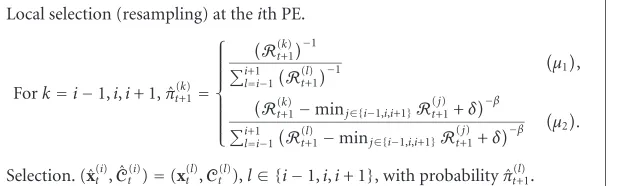
The latter observation is confirmed by the mean absolute deviation plot in Figure 2b. The deviation signal was com-puted as
et= 1
50 1 2
50
j=1
x1,t,j−xest1,t,j+x2,t,j−x2,estt,j, (53)
where jis the simulation number,xt,j =[x1,t,j,x2,t,j]T is the true position at time t, andxestt,j = [xest1,t,j,xest2,t,j]T is the cor-responding estimate obtained with the particle filter. We ob-serve that the CRPF algorithms withµ2attained the lowest
deviation and outperformed the auxiliary BF. Although it is not shown here, the auxiliary BF improved its performance as the sampling period was decreased,3and achieved a lower
deviation than the CRPFs for Ts ≤ 0.5 second. The reason is that, asTsdecreases, the correlation of the states increases due to the variation ofGu, and the BF exploits this statistical information better. Therefore, we can conclude that the BF can be more accurate when strong statistical information is available, and that the proposed CRPFs are more robust and
3Obviously, the BF will also deliver a better performance as the number of particlesMgrows. In fact, it can be shown [4] that the estimate of the posteriori pdf and its moments obtained from the BF converge uniformly to the true density and the true values of the moments. This means that, as M → ∞, the state estimates given by the BF become optimal (in the mean square error sense) and that for largeM, the BF will outperform the CRPF algorithm.
steadily attain a good performance for a wider range of sce-narios. This conclusion is easily confirmed with the remain-ing experiments presented in this section.
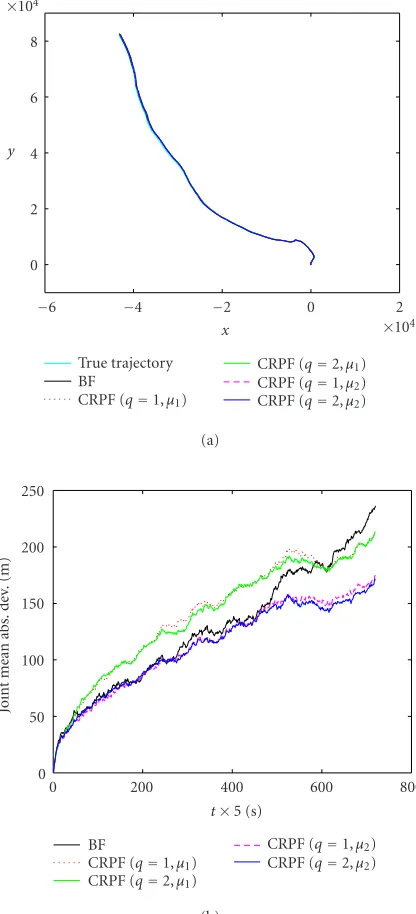
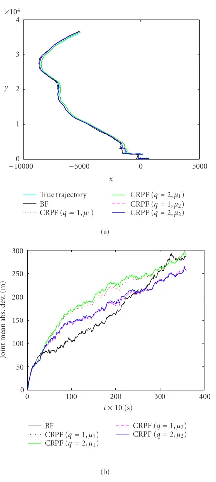
Figures3and4show the trajectories and the mean ab-solute deviations for the BF and CRPF algorithms when the sampling period was increased toTs=5 seconds andTs=10 seconds, respectively. Note that increasing Tsalso increases the speed measurement error. As before, the CRPF tech-niques withµ2outperformed the BF in the long term.
Because of its better performance, we also checked the behavior of the CRPF method that usesµ2for different
val-ues of parameterδ.Figure 5ashows the true position and the estimates obtained using three different values ofδ, namely, 0.1, 0.01, and 0.001, with fixedβ=2. All the algorithms ap-pear to perform similarly for the considered range of values. This is confirmed with the results presented inFigure 5bin terms of the mean absolute deviation. They also illustrate the robustness and stability of the method.
In the following, unless it is stated differently, the CRPF algorithm was always implemented withµ2and parameters
q =2,δ =0.01, andβ= 2. The sampling period was also fixed and wasTs=5 seconds.
5.2. Mixture Gaussian system and observation
noise—Gaussian BF
Figure 6shows the results (trajectory and mean deviation) obtained with the same system and observation noise distri-butions as inSection 5.1when the auxiliary BF (labeled as BF (Gaussian)) is mismatched with the dynamical system and models the noise processes with Gaussian densities:
p[ut]=N(0,
√
0.2I2),
p[wl,t]=N(0, 0.2), l=1, 2, 3.
(54)
It is apparent that the use of the correct statistical infor-mation is critical for the bootstrap algorithm (in the figure, we also plotted the result obtained when the BF used the true mixture Gaussian density—labeled as BF (M-Gaussian)). Note that the CRPF algorithm also drew the state particles from a Gaussian sequence of densities (seeSection 2.2), but it attained a superior performance compared to the BF.
5.3. Local versus multinomial resampling
1 0
−1
−2
−3
−4
×104 x
0 1 2 3 4
×104
y
True trajectory BF
CRPF (q=1,µ1)
CRPF (q=2,µ1) CRPF (q=1,µ2) CRPF (q=2,µ2) (a)
2000 1500
1000 500
0
t×2 (s) 0
50 100 150 200
Jo
int
mean
abs.
d
ev
.(
m)
BF
CRPF (q=1,µ1) CRPF (q=2,µ1)
CRPF (q=1,µ2) CRPF (q=2,µ2) (b)
Figure2: Mixture Gaussian noise processes.Ts = 2 seconds. (a)
Trajectory. (b) Mean absolute deviation.
can be observed inFigure 7. The CRPF with local resampling shows approximately the same performance as the BF with perfect knowledge of the noise statistics. Although it presents a slight degradation with respect to the CRPF with multi-nomial resampling, the feasibility of a simple parallel imple-mentation makes the local resampling method extremely ap-pealing.
5.4. Different estimation criteria
Figure 8 compares the trajectory and mean deviation of two CRPF algorithms that used different criteria to obtain the estimates of the state: the minimum cost estimate ˜xmin
t
2 0
−2
−4
−6
×104 x
0 2 4 6 8
×104
y
True trajectory BF
CRPF (q=1,µ1)
CRPF (q=2,µ1) CRPF (q=1,µ2) CRPF (q=2,µ2) (a)
800 600
400 200
0
t×5 (s) 0
50 100 150 200 250
Jo
int
mean
abs.
d
ev
.(
m)
BF
CRPF (q=1,µ1) CRPF (q=2,µ1)
CRPF (q=1,µ2) CRPF (q=2,µ2) (b)
Figure3: Mixture Gaussian noise processes.Ts = 5 seconds. (a)
Trajectory. (b) Mean absolute deviation.
(see (20)) and the mean cost estimate ˜xmean
t (see (21)). It is clear that both algorithms performed similarly and outper-formed the BF in the long term.
5.5. Laplacian noise
Finally, we have repeated our experiment by modeling the noises using Laplacian distributions, that is,
p[ut]=L
0,√0.5I2
= 1
0.5e −|ut|/0.5,
pwl,t
=0.3L(0, 0.5)= 1
0.5e
−|wl,t|/0.5, l=1, 2, 3.
5000 0
−5000
−10000
x 0
1 2 3 4
×104
y
True trajectory BF
CRPF (q=1,µ1)
CRPF (q=2,µ1) CRPF (q=1,µ2) CRPF (q=2,µ2) (a)
400 300
200 100
0
t×10 (s) 0
50 100 150 200 250 300
Jo
int
mean
abs.
d
ev
.(
m)
BF
CRPF (q=1,µ1) CRPF (q=2,µ1)
CRPF (q=1,µ2) CRPF (q=2,µ2)
(b)
Figure 4: Mixture Gaussian noise processes.Ts = 10 seconds.
(a) Trajectory. (b) Mean absolute deviation.
Figure 9depicts the results obtained for the BF with perfect knowledge of the probability distribution of the noise and the CRPF algorithm. Again, the proposed method attained better performance in terms of mean absolute deviation.
6. CONCLUSIONS
Particle filters provide optimal numerical solutions in prob-lems that amount to estimation of unobserved time-varying states of dynamic systems. Such methods rely on the knowl-edge of prior probability distributions of the initial state
2 0
−2
−4
−6
−8
×104 x
−6
−5
−4
−3
−2
−1 0 1
×104
y
True trajectory BF
CRPF (q=2,µ2,δ=0.1)
CRPF (q=2,µ2,δ=0.01) CRPF (q=2,µ2,δ=0.001)
(a)
800 600
400 200
0
t×5 (s) 0
50 100 150 200 250
Jo
int
mean
abs.
d
ev
.(
m)
BF
CRPF (q=2,µ2,δ=0.1) CRPF (q=2,µ2,δ=0.01) CRPF (q=2,µ2,δ=0.001)
(b)
Figure 5: Different δ values. Ts = 5 seconds. (a) Trajectory.
(b) Mean absolute deviation.
15 10
5 0
−5
×104 x
−5 0 5 10 15 20
×103
y
True trajectory BF (M-Gaussian) BF (Gaussian) CRPF (q=2,µ2)
(a)
800 600
400 200
0
t×5 (s) 0
50 100 150 200 250 300 350
Jo
int
mean
abs.
d
ev
.(
m)
BF (M-Gaussian) BF (Gaussian) CRPF (q=2,µ2)
(b)
Figure 6: Mixture Gaussian system and observation noise— Gaussian BF.Ts=5 seconds. (a) Trajectory. (b) Mean absolute
de-viation.
Since they do not assume explicit probabilistic models for the dynamic system, the proposed techniques, which have been termed CRPFs, are more robust than standard particle fil-ters in problems where there is uncertainty (or a mismatch with physical phenomena) in the probabilistic model of the dynamic system. The basic concepts related to the formu-lation and design of these new algorithms, as well as theo-retical results concerning their convergence, were provided. We also proposed alocal resamplingscheme that allows for simple implementations of the CRPF techniques with paral-lel VLSI hardware. Computer simulation results illustrate the
2 1
0
−1
×104 x
−10
−8
−6
−4
−2 0 2
×104
y
True trajectory BF
CRPF (multinomial) CRPF (local)
(a)
800 600
400 200
0
t×5 (s) 0
50 100 150 200 250
Jo
int
mean
abs.
d
ev
.(
m)
BF
CRPF (multinomial) CRPF (local)
(b)
Figure7: Local versus multinomial resampling.Ts = 5 seconds.
(a) Trajectory. (b) Mean absolute deviation.
robustness and the excellent performance of the proposed al-gorithms when compared to the popular auxiliary BF.
APPENDICES
A. CRPF AND STOCHASTIC APPROXIMATION
8 6
4 2
0
−2
×104 x
−2 0 2 4 6 8 10
×104
y
True trajectory BF
CRPF (mean) CRPF (min)
(a)
800 600
400 200
0
t×5 (s) 0
50 100 150 200 250
Jo
int
mean
abs.
d
ev
.(
m)
BF
CRPF (mean) CRPF (min)
(b)
Figure8: Different estimation criteria.Ts=5 seconds. (a)
Trajec-tory. (b) Mean absolute deviation.
In a typical problem addressed by SA, an objective func-tion that has to be minimized involves expectafunc-tions, for ex-ample, the minimization of E(Q(x,ψt)), where Q(·) is a function of the unknown x and random variables ψt. The problem is that the distributions of the random variables are unknown and the expectation of the function cannot be an-alytically found. To make the problem tractable, one approx-imates the expectation by simply dropping the expectation operator, and proceeding as ifE(Q(x,ψt)) =Q(x,ψt). Rob-bins and Monro proposed the following scheme that solves
6 4
2 0
−2
×104 x
−1 0 1 2 3 4 5
×104
y
True trajectory BF
CRPF
(a)
800 600
400 200
0
t×5 (s) 0
20 40 60 80 100
Jo
int
mean
abs.
d
ev
.(
m)
BF CRPF
(b)
Figure 9: Laplacian.Ts = 5 s. (a) Trajectory. (b) Mean absolute
deviation.
forxt:
ˆ
xt=xt−ˆ 1+γtQ
ˆ xt−1,ψt
, (A.1)
whereγtis a sequence of positive scalars that have to satisfy the conditionstγt= ∞,tγ2t <∞. In the signal processing literature, the best known SA method is the LMS algorithm.
it performs SA similarly to RM though by other means.4In
CRPF, the dynamics of the state are taken into account both through the propagation step and by recursively solving the optimization problem (25). Further research in CRPF from the perspective of SA can probably yield new and deeper in-sight of this new class of algorithms.
B. PROOF OFLEMMA 1
The proof is carried out in two steps. First, we prove the im-plication true under conditions (38)–(40) in order to complete the proof.
Straightforward manipulation of the inequality in (43) leads to the following equivalence chain that holds true for anyε,δ >0:
where we have exploited that
µtx(ti)
4Note, however, that the notion of inversion must be understood in a broad sense, sincefymay not necessarily be invertible and, even iff−1
y exists, it may happen thatytdoes not belong to its domain.
for the indicator function, we can write
µtxt(i)Mi=1\SMxtopt,ε
we can use the relationship [16, equation 4.4-5] to obtain
Pr
where we have used the fact that the supremum Sout does
not depend onMornM. When jointly considered, (B.9) and (B.10) yield the implication (B.1)⇒(B.2) and we only have to show that (B.1) holds true in order to complete the proof.
The expectation on the left-hand side of (B.1) can be computed by resorting to assumption (38), which yields, af-ter straightforward manipulations,
Substituting (B.11) into (B.1) yields
1−δ
C. PROOF OFTHEOREM 1
Using Lemma 1, we obtain that the set SM(xopt t ,ε) has (asymptotically) a unit probability mass after the propaga-tion step, that is,
lim
We write the upper bound on the right-hand side of (C.3) as a function of the radiusε: ∞, where # denotes the number of elements in a discrete set. Since limM→∞1/√M=0 and it is assumed thatC(·|yt) is
and, by exploiting the fact that the left-hand side of (C.2) does not depend onε, we can readily use (C.5) to obtain
which concludes the proof.
D. PROOF OFCOROLLARY 1
Whenλ=0,t(i)=πt(i)and, according toLemma 1,
for allε >0. Hence, we can write the mean state estimate (in the limitM→ ∞) as
and, therefore, the incremental cost of the mean state esti-mate can be upper bounded as
lim is minimal by definition, we find that
lim apply the same technique as in the proof ofTheorem 1and, takingε=1/√M, we obtain
which concludes the proof of the corollary.
ACKNOWLEDGMENTS
REFERENCES
[1] R. E. Kalman, “A new approach to linear filtering and predic-tion problems,” Transactions of the ASME—Journal of Basic Engineering, vol. 82, pp. 35–45, March 1960.
[2] B. D. O. Anderson and J. B. Moore, Optimal Filtering, Prentice-Hall, Englewood Cliffs, NJ, USA, 1979.
[3] S. Julier, J. Uhlmann, and H. F. Durrant-Whyte, “A new method for the nonlinear transformation of means and co-variances in filters and estimators,”IEEE Trans. on Automatic Control, vol. 45, no. 3, pp. 477–482, 2000.
[4] D. Crisan and A. Doucet, “A survey of convergence results on particle filtering methods for practitioners,” IEEE Trans. Signal Processing, vol. 50, no. 3, pp. 736–746, 2002.
[5] W. J. Fitzgerald, “Markov chain Monte Carlo methods with applications to signal processing,” Signal Processing, vol. 81, no. 1, pp. 3–18, 2001.
[6] J. S. Liu and R. Chen, “Sequential Monte Carlo methods for dynamic systems,”Journal of the American Statistical Associa-tion, vol. 93, no. 443, pp. 1032–1044, 1998.
[7] A. Doucet, S. Godsill, and C. Andrieu, “On sequential Monte Carlo sampling methods for Bayesian filtering,”Statistics and Computing, vol. 10, no. 3, pp. 197–208, 2000.
[8] N. Gordon, D. Salmond, and A. F. M. Smith, “Novel ap-proach to nonlinear and non-Gaussian Bayesian state estima-tion,”IEE Proceedings Part F: Radar and Signal Processing, vol. 140, no. 2, pp. 107–113, 1993.
[9] M. K. Pitt and N. Shephard, “Auxiliary variable based par-ticle filters,” inSequential Monte Carlo Methods in Practice, A. Doucet, N. de Freitas, and N. Gordon, Eds., pp. 273–293, Springer, New York, NY, USA, 2001.
[10] A. Doucet, N. de Freitas, and N. Gordon, Eds., Sequential Monte Carlo Methods in Practice, Springer, New York, NY, USA, 2001.
[11] M. L. Honig, U. Madhow, and S. Verd ´u, “Blind adaptive mul-tiuser detection,” IEEE Transactions on Information Theory, vol. 41, no. 4, pp. 944–960, 1995.
[12] J. R. Treichler, M. G. Larimore, and J. C. Harp, “Practical blind demodulators for high-order QAM signals,”Proceedings of the IEEE, vol. 86, no. 10, pp. 1907–1926, 1998.
[13] J. M´ıguez and L. Castedo, “A linearly constrained constant modulus approach to blind adaptive multiuser interference suppression,” IEEE Communications Letters, vol. 2, no. 8, pp. 217–219, 1998.
[14] T. L. Lai, “Stochastic approximation,”The Annals of Statistics, vol. 31, no. 2, pp. 391–406, 2003.
[15] M. Boli´c, P. M. Djuri´c, and S. Hong, “New resampling algo-rithms for particle filters,” inProc. IEEE International Confer-ence on Acoustics, Speech, and Signal Processing (ICASSP ’03), vol. 2, pp. 589–592, Hong Kong, April 2003.
[16] H. Stark and J. W. Woods, Probability and Random Processes with Applications to Signal Processing, Prentice-Hall, Upper Saddle River, NJ, USA, 3rd edition, 2002.
[17] M. Boli´c, P. M. Djuri´c, and S. Hong, “Resampling algorithms for particle filters suitable for parallel VLSI implementation,” inProc. 37th Annual Conference on Information Sciences and Systems (CISS ’03), Baltimore, Md, March 2003.
[18] F. Gustafsson, F. Gunnarsson, N. Bergman, U. Forssell, J. Jans-son, R. KarlsJans-son, and P.-J. Nordlund, “Particle filters for posi-tioning, navigation, and tracking,” IEEE Transactions on Sig-nal Processing, vol. 50, no. 2, pp. 425–437, 2002.
[19] H. Robbins and S. Monro, “A stochastic approximation
method,” Annals of Mathematical Statistics, vol. 22, pp. 400– 407, 1951.
Joaqu´ın M´ıguezwas born in Ferrol, Gali-cia, Spain, in 1974. He obtained the Licen-ciado en Inform´atica (M.S.) and Doctor en Inform´atica (Ph.D.) degrees from Universi-dade da Coru˜na, Spain, in 1997 and 2000, respectively. Late in 2000, he joined Depar-tamento de Electr ´onica e Sistemas, Univer-sidade da Coru˜na, where he became an As-sociate Professor in July 2003. From April to December 2001, he was a Visiting Scholar
in the Department of Electrical and Computer Engineering, Stony Brook University. His research interests are in the field of statistical signal processing, with emphasis on the topics of Bayesian analy-sis, sequential Monte Carlo methods, adaptive filtering, stochastic optimization, and their applications to multiuser communications, smart antenna systems, sensor networks, target tracking, and vehi-cle positioning and navigation.
M ´onica F. Bugalloreceived the Ph.D. de-gree in computer engineering from Univer-sidade da Coru˜na, Spain, in 2001. From 1998 to 2000, she was with the Departa-mento de Electr ´onica e Sistemas, the Uni-versidade da Coru˜na, where she worked in interference cancellation applied to mul-tiuser communication systems. In 2001, she joined the Department of Electrical and Computer Engineering, Stony Brook
Uni-versity, where she is currently an Assistant Professor, and teaches courses in digital communications and information theory. Her re-search interests lie in the area of statistical signal processing and its applications to different disciplines including communications and biology.
Petar M. Djuri´creceived his B.S. and M.S. degrees in electrical engineering from the University of Belgrade in 1981 and 1986, re-spectively, and his Ph.D. degree in electrical engineering from the University of Rhode Island in 1990. From 1981 to 1986, he was a Research Associate with the Institute of Nu-clear Sciences, Vinˇca, Belgrade. Since 1990, he has been with Stony Brook University, where he is a Professor in the Department of