DOI: 10.1534/genetics.106.062729
Multilevel Selection 2: Estimating the Genetic Parameters Determining
Inheritance and Response to Selection
Piter Bijma,* William M. Muir,
†,1Esther D. Ellen,* Jason B. Wolf
‡and
Johan A. M. Van Arendonk*
*Animal Breeding and Genetics Group, Wageningen University, 6709PG Wageningen, The Netherlands,†Department of Animal Science, Purdue University, West Lafayette, Indiana 47907-1151 and‡Faculty of Life Sciences,
University of Manchester, Manchester, M12 9PT, United Kingdom Manuscript received June 27, 2006
Accepted for publication October 26, 2006
ABSTRACT
Interactions among individuals are universal, both in animals and in plants and in natural as well as domestic populations. Understanding the consequences of these interactions for the evolution of pop-ulations by either natural or artificial selection requires knowledge of the heritable components underlying them. Here we present statistical methodology to estimate the genetic parameters determining response to multilevel selection of traits affected by interactions among individuals in general populations. We apply these methods to obtain estimates of genetic parameters for survival days in a population of layer chickens with high mortality due to pecking behavior. We find that heritable variation is threefold greater than that obtained from classical analyses, meaning that two-thirds of the full heritable variation is hidden to classical analysis due to social interactions. As a consequence, predicted responses to multilevel selection applied to this population are threefold greater than classical predictions. This work, combined with the quantitative genetic theory for response to multilevel selection presented in an accompanying article in this issue, enables the design of selection programs to effectively reduce competitive interactions in livestock and plants and the prediction of the effects of social interactions on evolution in natural populations undergoing multilevel selection.
I
NTERACTIONS among individuals are universal,both in animals and in plants and in natural pop-ulations as well as in domestic poppop-ulations. These inter-actions severely affect the direction and magnitude of responses to either natural or artificial selection (Dawkins 1982) and thus have important implications both for domestic breeding (Griffing1967; Muir1996) and for the outcome of evolution (Griffing1981a; Ridley1995; Goodnightand Stevens1997; Keller1999; Clutton -Brock2002).
With respect to agriculture, understanding how to reduce competitive interactions through artificial breed-ing is critical for global food security (Denison et al. 2003) and required to improve animal well-being in species currently used in agriculture, such as swine and poultry (Muir2003). Animal and plant breeders have been concerned about interactions among individuals, but have lacked direction as to methods to address these issues, and have been unsure as to the magnitude of the problem or even whether it exists at all. Griffing (1976a) observed that group selection could be used to ensure positive response to selection, but also noted that group selection was not very efficient. Determining
the impact of interactions for artificial selection pro-grams requires first of all knowledge of the genetic pa-rameters underlying the interactions. Such knowledge would enable optimization of breeding programs to maximize total genetic improvement of complex traits, but is currently lacking.
With respect to the study of evolution of interactions, one can distinguish two approaches: the adaptionist ap-proach (e.g., Hamilton1964a; Williams1966; Maynard -Smith1974; Wilsonand Sober1989; Westet al.2002) and the genetic approach (Williams and Williams 1957; Griffing1967, 1981a; Wright1968, 1977; Wade 1979; Mooreand Boake1994; Goodnightand Stevens 1997; Roff 1997; Goodnight 2005). The adaptionist approach focuses on explaining existing phenotypic adaptations, whereas the genetic approach focuses on modeling ongoing evolution by natural selection. Adap-tionists treat the current population as an end point and seek to explain current phenotypes by considering whether they are evolutionary stable (Maynard-Smith 1974). Hence, they implicitly assume that current trait values are optimal, meaning that traits have no heritable covariance with fitness. Geneticists, in contrast, take the opposite approach by assuming that all traits are herit-able. With respect to behavioral traits, the adaptionist
approach has so far had the most impact (Moore
and Boake 1994; Goodnight 2005). In many cases,
1Corresponding author:Department of Animal Science, 1151 Lilly Hall,
Purdue University, W. Lafayette, IN 47907-1151. E-mail: [email protected]
however, it is unknown whether or not traits in natural populations have a heritable covariance with fitness, which is particularly true for complex traits related to behavior.
In general, response to selection depends on the herit-able variation in the traits of interest. Classical quanti-tative genetic theory states that response to selection equals the product of heritability and the selection differential,R¼h2S, a result known as the ‘‘breeder’s equation’’ (Lynchand Walsh1998). Griffing(1967, 1968a,b, 1969, 1976a,b, 1981a,b) and later develop-ments of others (Mooreet al.1997; Wolfet al.1998), however, showed that interactions among individuals involve additional heritable components. The accom-panying article (Bijmaet al.2007, this issue) shows that interactions among individuals may create substantial additional heritable variation. Selection among individ-uals does not capture this additional variation, but selec-tion acting on higher levels of organizaselec-tion, such as a group, captures the full heritable variation. Thus, knowl-edge of the amount of heritable variation hidden due to social interactions is critical to understand and predict consequences of multilevel selection.
At present, there is very little information on the amount of heritable variation hidden due to social interactions. The large responses observed in selection experiments applying selection among groups, how-ever, provide indirect evidence for substantial hidden variation (Craig and Muir 1996; Muir 1996; see Goodnightand Stevens1997 for a review). It is clear from those experiments (see Table 1 in Goodnightand Stevens1997), and from results presented herein, that multilevel selection could result in the next major advance in both domestic plant and animal breeding. Full utilization of heritable interactions and multilevel selection in artificial breeding, and a better under-standing of the impacts of interactions for evolution by natural selection, however, requires methodology to estimate the relevant genetic parameters in general populations.
Here we present statistical methodology to estimate the genetic parameters of traits affected by interactions, for interactions among any number of individuals in general nondesigned populations with any degree of relatedness among individuals. Next, we present esti-mates for the amount and composition of the total herit-able variation for survival days in a population of layer chickens (Gallus gallus) and investigate the prospects of using multilevel selection and relatedness to improve survival in that population, by utilizing the total herita-ble variation.
BACKGROUND
This section briefly summarizes the quantitative genetic theory of multilevel selection as presented in Bijmaet al.(2007).
Model: We consider a population in which interac-tions occur within ‘‘groups’’ ofn individuals each and affect phenotypic values of individuals. In classical quantitative genetic theory, the phenotypic trait value of an individual,P, is the sum of a heritable component,
A, referred to as ‘‘breeding value’’ and a residual com-ponent, E, referred to as ‘‘environment’’:P ¼A 1 E. With interactions among n individuals, however, the observed phenotypic trait value of an individual is due to two unobserved phenotypic effects: a direct effect originating from the focal individual and the sum of the associative effects originating from of each of itsn1 group members (Griffing 1967). Associative effects may be interpreted as heritable environmental effects provided by associates to the focal individual (Wolf 2003). Both phenotypic direct and associative effects are the sum of a heritable component (A) and a nonherit-able component (E), so that the observed phenotypic trait value of an individual is given by
Pi ¼AD;i1ED;i1
Xn
i6¼j
AS;j1
Xn
i6¼j
ES;j ð1Þ
(Griffing1967), in whichidenotes the focal individual andj one of its associates (i.e., group members). The first two terms in Equation 1 represent effects due to the focal individual; the last two terms represent the effects due to itsn1 associates. The effectAD;i is the direct breeding value (DBV) and ED,i is the direct nonherit-able value of individuali, whereasAS;j is the associative breeding value (SBV) andES,jthe associative nonherit-able value of associatej. The DBV and the SBV represent the heritable components underlying the observed phenotypes.
Note that nonheritable associative effects, indicated by Pni6¼jES;j in Equation 1, may contribute to the ob-served phenotype. This is because the full associative effect of an individual is a phenotypic effect, which may contain both heritable and nonheritable components. The genes of an individual do notdirectlyaffect the as-sociates; the associates experience a phenotype. We em-phasize those nonheritable associative effects, because they modify the statistical model required to obtain unbiased estimates of genetic parameters (see below).
Heritable variation:Because each individual interacts withn 1 associates, the total heritable impact of an individual on the population mean, referred to as its total breeding value (TBV), equals the sum of its DBV andn1 times its SBV: TBVi¼DBVi1(n1)SBVi. Response to selection equals the change per generation of the TBV. Hence, the TBV is a generalization of the classical breeding value, to account for interactions. The total heritable variation available for response to selec-tion, therefore, equals the variance of the TBV,
s2TBV¼s2A
D12ðn1ÞsADS1ðn1Þ
2s2
(Bijmaet al.2007), in whichs2
ADis the variance of DBV,
s2
ASis the variance of SBV, andsADSis the covariance
be-tween DBV and SBV. The sign of the covariance bebe-tween DBV and SBV is a measure of competitionvs. cooper-ation. Negative sADS may be interpreted as ‘‘heritable
competition,’’ in the sense that individuals with positive breeding values for their own phenotype (DBV) have on average a negative heritable impact on the phenotypes of their associates (SBV). Conversely, positivesADS may
be interpreted as ‘‘heritable cooperation.’’
Classical quantitative genetic methodology to esti-mate additive genetic variances of traits rests on similar-ity of phenotypes’ relatives. Associative breeding values of individuals, however, are not expressed in their own phenotypes, but in the phenotypes of their associates. Thus only the variance of DBV surfaces in classical ana-lyses; the remaining part of the full heritable variance, 2ðn1ÞsADS1ðn1Þ
2s2
AS, is hidden. Depending on
group size and the heritability of interactions, this hid-den heritable variance may be substantially larger than the variance of DBVs. In those cases, classical methods will substantially underestimate the total heritable vari-ation. With specific family structures, the SBV may also be confounded with the DBV (seediscussionand Wolf 2003), which would make the result of classical analyses an inaccurate estimate of even the direct genetic vari-ance. The total heritable variation (Equation 2) does not depend on relatedness among associates. This is because all components of the TBV of an individual refer to its own genes. (See Bijmaet al.2007 for the effect of pop-ulation structure.)
Response to selection: In classical quantitative ge-netic theory, response to selection is in the same direc-tion as selecdirec-tion pressure; heritability is merely a scaling factor affecting the magnitude of response, not its direc-tion. With interactions among individuals, however, not only the magnitude, but also the direction of response depend on the genetic parameters (Griffing 1967; Kirkpatrickand Lande1989; Mooreet al.1997). To illustrate this phenomenon, we consider response to se-lection among unrelated individuals, which follows from substituting r ¼g¼ 0 into Equation 5 of Bijma et al. (2007), giving DP¼ s2
AD1ðn1ÞsADS
ði=sCÞ, in whichi=sCis the selection gradient. (See also Griffing 1976a.) This result shows that the direction of response depends on the covariance between DBV and SBV (sADS).
Strong competition,i.e., large and negativesADS, will yield
response in the direction opposite to the direction of se-lection. With interactions, therefore, the genetic param-eters play a key role in the outcome of selection; they are no longer merely a scaling factor.
METHODS
Powerful methods to estimate genetic parameters have been developed in the field of animal breeding (Henderson 1950; Lynch and Walsh 1998). Those
methods have become known as ‘‘animal models’’ and have recently been introduced into other fields in biol-ogy (Kruuket al.2003). In the following, we extend the animal model to account for interactions. Particular emphasis is given on the proper inclusion of nonherit-able associative effects.
In its basic form,i.e., in the absence of interactions, an animal model is given by
y¼Xb1Za1e; ð3Þ
in which yis a vector of observed phenotypes; b is a vector of so-called ‘‘fixed’’ effects, with incidence matrix
Xlinking observations on fixed effects;ais a vector of breeding values, with incidence matrix Zlinking phe-notypic values of individuals to their breeding values; andeis a vector of residuals. Fixed effects inbaccount for systematic nongenetic differences among observa-tions, such as age or treatment effects. Covariance struc-tures of model terms are: Var½a ¼As2
A, in whichAis a matrix of coefficients of relatedness between individuals ands2
Athe variance of breeding values (which is to be estimated), and VarðeÞ ¼Is2
e, in whichIis an identity matrix (Ijj¼1 andIjk¼0) ands2e the residual variance. The Zaterm in the model, together with its variance structure, accounts for the genetic covariances between all observations.
To account for interactions in the animal model, we investigated the structure of the covariances between observations that arise from Equation 1 and formulated a statistical model that yields the same covariance structure. (The derivation is in the next section.) The resulting statistical model is summarized as
y¼Xb1ZDaD1ZSaS1e; ð4Þ
in whichaDis a vector of DBVs, with incidence matrixZD
linking phenotypic values of individuals to their DBV;aS
is a vector of SBVs, with incidence matrix ZS linking
phenotypic values of individuals to the SBVs of their as-sociates; ande is a vector of residuals. The covariance structure of genetic terms is Var aD
aS
¼C5A, where
C¼ s
2
AD sADS
sADS s2A S
" #
and 5 indicates the Kronecker product of matrices. (Note that the elementyiofyin Equation 4 corresponds to Pi in Equation 1.) This fully describes the genetic components of the covariance between observations.
The covariance structure of the residual term of the model,e, can be derived using Equation 1 and is given by
VarðeÞ ¼Rs2e;
withRii¼1;
Rij¼r;iandjare in the same group;i6¼j;
(see next section for derivation), in whichs2
e ¼s2ED1
ðn1Þs2
ES and r¼ 2sEDS1ðn2Þs
2
ES
=s2
e, which is the correlation between residuals of group members. Together, Equations 4 and 5 fully describe the covar-iance structure that arises from Equation 1.
Derivations: This section describes the derivations of Equations 4 and 5. Consider two individuals,i with group members denoted byjandkwith group members denoted byl. The covariance between phenotypes ofi
andkfollows from substituting Equation 1 for bothPi andPk, giving CovðPi;PkÞ ¼CovðAD;i1
P
j6¼iAS;j;AD;k1
P
l6¼kAS;lÞ1CovðED;i1
P
j6¼iES;j;ED;k1
P
l6¼kES;lÞ,which consists of a genetic and an environmental component. Analogous to the basic animal model, we account for the genetic components by including direct and asso-ciative breeding values in the model, together with their covariance structure. This yields Equation 4. For exam-ple, in Equation 4, theith element ofycorresponds to
Pi, theith element ofZDaDcorresponds toAD,i, theith element of ZSaScorresponds to Pj6¼iAS;j, and theith element ofecorresponds toED;i1
P
j6¼iES;j. As usual in an animal model, we account for covariances between breeding values inaD andaSby incorporating the
re-latedness matrixAin the statistical analyses. (See below and the mixed-model equations in Muir2005.)
What remains to be done is the covariance structure of the vector of residuals e. The covariance between residuals ineoriginates from the environmental com-ponent of the covariance between observations and can be partitioned into Covðei;ekÞ ¼CovðPi;PkÞenv:¼
CovðED;i1 Pj6¼iES;j;ED;k1 Pl6¼kES;lÞ¼CovðED;i;ED;kÞ1 CovðED;i;Pl6¼kES;lÞ1CovðPj6¼iES;j;ED;kÞ1CovðPj6¼iES;j;
P
l6¼kES;lÞ. As usual in quantitative genetics, we assume that E-terms of distinct individuals are independent. (Environmental effects common to multiple individuals are accounted for by the fixed effects Xb.) Thus a nonzero residual covariance occurs only when it in-volves the same individual, which happens either wheni
andkare the same individual or wheniandkare group
members. When i and k are the same individual,
Covðei;ekÞ ¼s2e¼VarðED1
P
n1ESÞ ¼sE2D1ðn1Þs
2
ES,
which is the residual variance. The first term is due to the direct effect of the individual itself, and the second term is due to itsn1 group members. Wheniandkare group members, their residuals are correlated for two reasons. First, for groups larger than two, iand kwill haven2 group members in common, and thus they haven 2 identical associative effects in their pheno-type, giving CovðPj6¼iES;j;Pl6¼kES;lÞ ¼ ðn2Þs2ES.
Sec-ond, the direct effect of i is expressed in its own phenotype, whereas the associative effect ofiis expressed in the phenotype ofk, and vice versa fork. As with any two traits of a single individual, the direct and associa-tive effect originating from a single individual may be correlated Walsh (Lynch and Walsh 1998), giving CovðED;i;
P
l6¼kES;lÞ1Covð
P
j6¼iES;j;ED;kÞ¼CovðED;i;ES;iÞ1 CovðES;k;ED;kÞ ¼2sEDS. Thus the full covariance between
residuals of group members equals 2sEDS1ðn2Þs
2
ES.
The sEDS represents the nonheritable relationship
be-tween the direct and associative effect of an individual and is a nonheritable measure of competitionvs. coopera-tion (analogous tosADS, see above). A negativesEDS may,
for example, arise from variation in the juvenile environ-ment experienced by individuals. Individuals having ex-perienced good (bad) environments may be more (less) competitive, in which case they will have higher (lower) phenotypic values at the expense (to the advantage) of their associates. In Equation 5, we accounted for the non-genetic covariance between group members by fitting the correlationrbetween records of group members.
Experimental design for application:The use of Equa-tions 4 and 5 does not require a specific experimental design; groups may be composed of any combination of related and/or unrelated individuals and may vary in size. To calculate the relationship matrixA, information on at least one generation of family relationships will be required, so that one can distinguish full sibs, half sibs, and unrelated individuals. Information on more gen-erations of pedigree, which provides information on more distant relationships, will add to the accuracy of results, but is not required for application. With groups of equal size, there will be no information in the data to separatesEDS ands2
ES, because different combinations
of those two parameters may yield an identical residual correlation. The inability to estimatesEDS ands2
ES with
equal group size is no problem, because the residual correlation itself, which included these components as part of a ratio, is estimable and sufficient in the analysis to avoid bias in the estimates of the genetic parameters. There are population structures from which the param-eters of interest cannot be estimated. (Seediscussion on the work of Wolf2003).
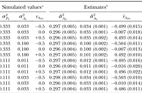
We used Monte Carlo simulations to validate our sta-tistical methodology (appendix). Table 1 shows that estimated genetic parameters obtained from simulated data are unbiased; true values of genetic parameters are within63 standard errors of mean estimated values in all cases. These results confirm that Equations 4 and 5 correspond to the covariance structure that arises from Equation 1 and that there is no need for a specific structure of the family relationships within and between groups.
APPLICATION
Material: The methodology presented above was applied to analyze mortality in a commercial population of layer chickens. Field data on this population were provided by Hendrix Genetics and consisted of obser-vations on survival days of a single generation of 3800 hens bred from 36 sires and 287 dams, which had been
mated at random. Each sire had been mated to 8
offspring. Five generations of pedigree were included in the calculation of the matrix of relatedness (A).
Mortality in commercial chicken populations is largely due to cannibalistic pecking behavior (e.g., Craigand Muir 1996). The direct effect of an individual is, therefore, related to its ability to survive by avoiding being pecked, whereas its associative effect measures its effect on survival of its cage members, which is closely related to its own pecking behavior. In commercial egg production, individuals are frequently beak trimmed, to reduce mortality due to pecking behavior. In this data set, however, individuals had not been beak trimmed, which will be obligatory in the European Union from 2011 onward.
Data consisted of four age groups of approximately equal numbers of hens, differing by 2 weeks of age each. At an age of 20 weeks, individuals were allocated ran-domly to 950 standard commercial battery cages, four individuals per cage. Due to chance, some cages con-tained full or half sibs, but most cages concon-tained un-related individuals only. Facilities consisted of eight rows of cages. Each row was 40 cages long and consisted of 3 cages on top of each other, giving 120 cages per row. The eight rows were grouped into four double rows; both rows of a double row were put with the backs against each other. Each age group was allocated to a
single double row. Back fences of cages consisted of latticework allowing limited contact between ‘‘backdoor neighbors,’’ i.e., between the individuals of two corre-sponding cages, each in one of the two rows of a double row. Adjacent cages in the same row were separated by a closed fence fully preventing contact. Individuals were kept 60 weeks and culled at an age of 80 weeks. Survival (0/1) was recorded daily on all individuals. For each individual, survival days were defined as age at death in days. Individuals surviving until 80 weeks of age had 80 3 7 ¼ 560 survival days. Fifty-four percent of individuals survived until 80 weeks of age. Mean survival time was 454 days, with a standard deviation of 122 days. Inspection of dead hens showed that the vast majority of chickens had died due to being pecked. This observa-tion was supported by previous data on beak-trimmed individuals of the same line kept in the same facilities, which showed substantially lower mortality (,10%). Thus the absence of beak trimming substantially ampli-fied the consequences of social interactions.
Data were analyzed with Equations 4 and 5 as a model, using restricted maximum likelihood (REML) (Pattersonand Thompson1971) as implemented in the ASReml software package (Gilmour et al. 2002). The model included a fixed effect for each combina-tion of row (1 through 8) and level (top, middle, and bottom) of the cage and for the number of surviving birds in the back cage, to account for a possible as-sociative effect due to the backdoor neighbors. As usual with an animal model, this analysis directly yields esti-mates of the parameters of interest and utilizes the full data.
Results: When using a conventional model without associative effects, estimated heritability for survival days in the chicken line was 6.7%, which is in the range com-mon for survival traits in livestock (Table 2; Beaumont
et al. 1997; Carlenet al.2005; Gitterleet al.2005). The total heritable variance estimated from the full model (Equations 2, 4, and 5), however, was 2742 days2, which corresponds to 20% of the phenotypic variance. This result indicates a ‘‘heritability’’ threefold greater than that obtained using classical methods,i.e., 20%vs. 6.7%. Two-thirds of the heritable variation, therefore, is due to social interactions among individuals and is hidden from classical analyses.
At first glance, one might expect direct and associa-tive effects for mortality due to pecking behavior to be negatively correlated, because dominant individuals may kill others and survive themselves. However, we found a small but nonsignificant positive correlation of
10.28 (P¼0.016), suggesting that individuals benefit from not harming others. In this population, there seems to be mutual benefit of behaving peacefully and a mutual cost of behaving aggressively. A positive co-variance between DBV and SBV increases the total heritable variation (Equation 2) and therefore increases the potential of the population to respond to selection.
TABLE 1
Validation of statistical methodology
Simulated valuesa Estimatesb
s2
PS s
2
AS rADS sˆ
2
AD sˆ
2
AS ^rADS
0.333 0.033 0.5 0.297 (0.005) 0.034 (0.001) 0.499 (0.015) 0.333 0.033 0.0 0.296 (0.005) 0.035 (0.001) 0.007 (0.018) 0.333 0.033 10.5 0.296 (0.005) 0.035 (0.002) 0.493 (0.014) 0.333 0.100 0.5 0.297 (0.004) 0.100 (0.002) 0.504 (0.011) 0.333 0.100 0.0 0.296 (0.004) 0.100 (0.002) 0.007 (0.013) 0.333 0.100 10.5 0.297 (0.005) 0.101 (0.002) 0.492 (0.010) 0.111 0.011 0.5 0.297 (0.004) 0.012 (0.001) 0.495 (0.016) 0.111 0.011 0.0 0.296 (0.004) 0.011 (0.001) 0.016 (0.020) 0.111 0.011 10.5 0.297 (0.004) 0.012 (0.001) 0.496 (0.022) 0.111 0.033 0.5 0.298 (0.005) 0.034 (0.001) 0.503 (0.010) 0.111 0.033 0.0 0.296 (0.004) 0.033 (0.001) 0.010 (0.014) 0.111 0.033 10.5 0.297 (0.004) 0.033 (0.001) 0.486 (0.011)
a
Simulated populations consisted of 250 sires, 500 dams, and data on 20 offspring per dam. Individuals were kept in 2500 groups of four individuals each. Simulated genetic parameters were:s2
PD¼1:0, s
2
AD¼0:3; s
2
PS was either 33 or 11% of s2
PD, representing large or small associative effects;
s2
ASwas either 10 or 30% ofs
2
PS, representing low or high her-itability of associative effects; the genetic correlation between DBV and SBV (rADS) was0.5, 0, or10.5 and the nongenetic correlation (rEDS) equaled the genetic correlation. Fifty repli-cates were simulated for each population structure and five generations of pedigree were included in the calculation of the relationship matrix (A).
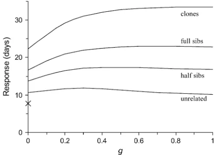
Figure 1 shows predicted responses to multilevel se-lection applied to the chicken population, using equa-tions presented in Bijmaet al.(2007). (Details and an example of calculation are in theappendix.) In Figure 1, the strength of multilevel selection is indicated by a factor g, where g ¼ 0 represents selection among in-dividuals,g¼1 represents selection among groups, and values ofgbetween 0 and 1 represent a mix of selection among individuals and groups (Bijma et al. 2007). Classical theory suggests a response of only 7.8 days of survival. Predictions accounting for heritable interac-tions, however, yield substantially higher responses. Se-lection among individuals applied to a population composed of groups of unrelated individuals yields an expected response of11 days of survival (g¼0,r¼0). Mild multilevel selection applied to a population com-posed of groups of full sibs more than doubles the predicted response (g $ 0.3, r ¼1
2). The maximum
response that can be obtained equals 23 days (g¼0.6– 0.8 andr ¼1
2), which is nearly threefold greater than
suggested by classical theory. (Clones do not occur in reality.) The lines in Figure 1 are curved, which indicates that a degree of between-group selection (g) that max-imizes response exists, which was also observed by Griffing. This value of g may be applied in artificial breeding programs, where the aim is to maximize response to selection. Note that results in Figure 1 are specific to the chicken population and to the environ-ment in which it was kept, such as the density of housing; other populations may have other genetic parameters and other relationships among relatedness, multilevel selection, and response. Results in Figure 1 should,
therefore, not be taken to conclude that relatedness has a bigger impact than multilevel selection in general.
DISCUSSION
We have presented methodology to estimate the genetic parameters of traits affected by interactions among individuals of any degree of relatedness in gen-eral populations. The Monte Carlo simulations confirm that our methods yield unbiased results. In an accom-panying article (Bijmaet al.2007, this issue), we provide the quantitative genetic theory for the consequences of multilevel selection. That article shows that, in theory, heritable interactions may have substantial consequen-ces, such as the existence of considerable yet hidden heritable variation. This article provides the methods to estimate the genetic parameters required for applying the theory. Analysis of the chicken population revealed a threefold greater heritable variation and potential response to selection than estimated by classical meth-ods. These findings demonstrate the relevance of our theoretical work for real populations.
Together, both articles provide testable predictions of response to multilevel selection in general populations. These predictions may be used to optimize artificial breeding programs for heritable traits that have never-theless been refractory to selection among
individ-uals (Teichertcoddington and Smitherman 1988;
Vangen1993; Kruuket al.2001; Muir2005). Even for traits not refractory to selection, responses obtained in current selection programs are most likely less than what can be achieved by accounting for interactions. For example, results for the chicken population show that
TABLE 2
Estimated genetic parameters in a population of laying hens
Parameter
Classical analysesa
Equations 4 and 5
Phenotypic variance 13,706b 13,725c Direct genetic variance 917*** 960*** Associative genetic variance — 132**
DA genetic covariance — 99 NS
Residual correlation 0.12*** 0.09***
% heritable variationd 6.7% 20.0%
Significance levels were obtained from likelihood-ratio tests comparing the full model to the model omitting the term of interest. **P,0.01; ***P,0.001; NS, not significantly dif-ferent from zero; DA, direct–associative.
aIn this analysis, the termZ
SaSwas omitted from the model
(Equation 4). bObtained as ˆs2
P ¼sˆ
2
AD1sˆ
2
e.
cObtained as ˆs2
P ¼sˆ
2
AD1ðn1Þsˆ
2
AS1sˆ
2
e.
dThe percentage of heritable variation was ˆs2 TBV=sˆ
2
P3
100%, in which ˆs2
TBVwas obtained from Equation 2 by
replac-ing true values by the correspondreplac-ing estimates, givreplac-ing 9601
2333991323132¼2742 days2. (In the classical analyses ˆ
s2
TBV¼sˆ 2
AD).
Figure 1.—Predicted responses to selection for the trait
survival days in the chicken population, with groups consist-ing of one of four types of relatives. Predictions are obtained using results in Table 2 and a selection intensity of 1 unit ði¼1Þ. (Methods are in theappendix). The gdenotes the
strength of multilevel selection. The prediction from classical theory is ih2s
P¼0:0673
ffiffiffiffiffiffiffiffiffiffiffiffiffiffiffi
13;706
p
optimal multilevel selection will yield a response twofold greater than that of individual selection (23vs.11 days, Figure 1). The additional response to selection is ex-pected to be even greater for situations where the covar-iance between direct and associative effects is negative,
e.g., in situations with competition for limited resources. In the field of evolutionary biology, our methods may be used to quantify the potential of social traits to evolve in response to natural selection acting on multiple levels and also to investigate whether social traits in current populations show a heritable covariance with fitness, in which case they would respond to natural selection, indicating that current trait values deviate from evolu-tionary stable state trait values.
In stark contrast to classical theory, the total heritable variance (s2
TBV) can in principle exceed the observed
phenotypic variance. Consider, for example, groups con-sisting of unrelated individuals. In that case, the vari-ance among observed phenotypes equals s2
AD1s
2
ED1
ðn1Þðs2
AS1s
2
ESÞ(Equation 1;
appendix), whereas the
total heritable variance equals s2
TBV¼s
2
AD12ðn1Þ
sADS1ðn1Þ
2s2
AS (Equation 2). Comparing both
ex-pressions shows thats2
TBV is most likely to exceed the
phenotypic variance when groups are large, associative effects are largely heritable, and the covariance between DBV and SBV is positive. For example, with n ¼ 10, s2
PD¼1;s
2
PS ¼0:2, heritable variances of direct and
as-sociative variances equal to 50% of the corresponding phenotypic variances, and sADS ¼0, the phenotypic variance equals 111130.2¼3.2, whereas the heritable variance equals 0.519230.1¼8.6. This example shows that interactions can in principle cause the heritable variance to exceed the phenotypic variance. Whether this occurs in real populations has not yet been inves-tigated to our knowledge.
Previous work on the genetic background and evolu-tion of social effects (Hamilton1963, 1964a,b; Wolf
et al.1998; Wolf2003) has focused predominantly on pairs of individuals, whereas the current approach applies to groups of any number of individuals. For certain types of interactions, such as maternal effects, it is obvious to consider only two individuals. Results for two individuals, however, do not generalize to larger groups. In larger groups, the variance of SBVs becomes the dominant term, both for response to selection and for the total heritable variation (Equation 2) (Bijma
et al.2007). The total heritable variation contains a term
ðn1Þ2s2
AS (Equation 2), which increases rapidly with
group size, indicating that populations consisting of large groups may contain substantially more heritable variation than populations consisting of small groups.
The impact of group size on the heritable variation and on response to selection depends critically on the relationship between the variance of SBVs and group size. Depending on the nature of the trait, the variance of SBVs may or may not decrease with group size, and consequently the total heritable variance may either
in-crease rapidly with group size or maintain a stable value (Bijmaet al.2007). Knowledge of the relationship be-tween group size and the heritable variance would provide insight into the contribution of group augmen-tation to the evolution of social behaviors (Clutton -Brock2002). For populations consisting of groups of different sizes, the methodology presented here can be extended to examine that relationship (not shown).
In comparison to other methods, Wolf(2003) pre-sented an experimental design and a statistical method to estimate direct and associative genetic (co)variances in populations consisting of groups of two individuals and presented results for body length in Drosophila melanogaster. Results indicated an associative genetic variance of approximately half the direct genetic vari-ance and a strong negative genetic correlation of0.85 between direct and associative effects. In the experi-mental setup, flies were kept in pairs of individuals that were full sibs, half sibs, or unrelated. With unrelated individuals, the same two half-sib families were always combined in a pair. Dams were nested within sires; each sire was mated to exactly two dams and each dam to a single sire only. Data were analyzed using a sire and dam-within-sire model (referred to as ‘‘sire–dam model’’ in the following), and residuals were treated as indepen-dent, both within and between tubes (i.e., groups). Direct and associative genetic (co)variances were esti-mated using an ANOVA method, in which estiesti-mated sire and dam variances were equated to their expectations. Further details are in Wolf(2003). We investigated this experimental design using Monte Carlo simulation of the population structure of Wolf (2003). Simulated populations were analyzed using either Equations 4 and 5 or a sire–dam model. To our surprise, results from Equations 4 and 5 indicated that the associative genetic variance could not be estimated with this experimental design, whereas estimates from a sire–dam model were severely biased. To determine for certain whether or not the associative genetic variance can be estimated in this experimental design, we examined in detail the expec-tations of the sire and dam variances presented in Wolf(2003), which revealed that they are incomplete (appendix). Investigation of the complete expectations confirmed that the associative genetic variance cannot be estimated using the experimental design proposed by Wolf(2003). Moreover, it revealed that a sire–dam model is unsuitable for estimating direct and associative genetic (co)variances, because the true expectations of sire and dam ‘‘variances’’ can take negative values (because they are, in reality, covariances that, unlike variances, are not restricted to nonnegative values). Indeed, the expected sire variance would take a negative value when estimates presented in Wolf(2003) would be the true values (appendix). Results presented in Wolf (2003), therefore, may need to be reconsidered.
genetic variances presented in Wolf (2003). To illus-trate the potential consequences of assuming indepen-dent residuals, we reanalyzed the data on the chicken line by fitting both direct and associative genetic effects according to Equation 4, but replacing Equation 5 by VarðeÞ ¼Is2
e. A likelihood-ratio test (Wald 1943; Lynch and Walsh 1998) strongly favored correlated residuals (P , 0.001). Results (not shown) indicated severely affected estimates of the genetic parameters, which increased by 37% for the variance of DBV, by 175% for the variance of SBV, and by 360% for the covariance between DBV and SBV, yielding a total heritable variation 2.6-fold greater than the original result (7294 instead of the 2742 days2in Table 2). These results demonstrate that even a very small residual correlation (ˆr¼0:09, Table 2) may substantially bias the estimated genetic parameters and illustrate the need to allow for nonheritable associative effects in the statistical analysis.
Muir(2005) presented similar methodology to esti-mate direct and associative genetic (co)variances in gen-eral populations. With respect to genetic components, our model (Equation 4) is the same as that of Muir (2005). However, Muir (2005) assumed that sE
DS ¼0.
This would imply that r¼ ½ðn2Þs2
ES=½ðn1Þs
2
ES1
s2
ED, which is necessarily positive. That assumption is
likely to be violated, because an environmental effect that increases its own direct effect will most likely have a negative impact on others (except for altruistic effects). Here we presented the general solution, which obeys the basic quantitative genetic assumptions that (i) pheno-typic values are the sum of both genetic and environ-mental values and (ii) phenotypic covariances are the sum of both genetic and environmental covariances.
The above considerations show that the choice of proper models and statistical methods is critical to the outcome and biological interpretation of results. Fur-thermore, the analysis of the experimental design of Wolf (2003) shows that for certain population struc-tures the genetic parameters of interest cannot be estimated. That result is not specific to our statistical methodology, but holds in general. The experimental design used in Wolf (2003) yields a covariance struc-ture between observations that is independent of the relative magnitudes of direct and associative genetic variances (appendix). To estimate genetic parameters of traits affected by interactions, we suggest the use of animal models and random composition of groups. Animal models directly include the animal component, instead of underlying components as sire and dam, and are a powerful tool for data analyses in both natural and domestic populations (Kruuk 2004). Application of animal models does not require designed populations and avoids the complexity of deriving expectations of sire and dam variances and the risk of obtaining estimates outside the parameter space, which may occur in ANOVA-based methods.
We thank Henk Bovenhuis, Bart Ducro, Charles Goodnight, Han Mulder, Jeroen Visscher, Patrick Wissink, and Addie Vereijken for stimulating discussions during the development of this work and Hendrix Genetics for providing the data on laying hens. Part of this work was funded by Senter Novem, The Netherlands.
LITERATURE CITED
Beaumont, C., N. Millet, E. LeBihanDuval, A. Kipiand V. Dupuy,
1997 Genetic parameters of survival to the different stages of embryonic death in laying hens. Poult. Sci.76:1193–1196. Bijma, P., W. M. Muirand J. A. M. VanArendonk, 2007 Multilevel
selection 1: quantitative genetics of inheritance and response to selection. Genetics175:277–288.
Carlen, E., M. D. Schneiderand E. Strandberg, 2005 Comparison
between linear models and survival analysis for genetic evaluation of clinical mastitis in dairy cattle. J. Dairy Sci.88:797–803. Clutton-Brock, T., 2002 Behavioral ecology—breeding together:
kin selection and mutualism in cooperative vertebrates. Science
296:69–72.
Craig, J. V., and W. M. Muir, 1996 Group selection for adaptation
to multiple-hen cages: beak-related mortality, feathering, and body weight responses. Poult. Sci.75:294–302.
Dawkins, M., 1982 The Extended Phenotype. W. H. Freeman, San
Francisco.
Denison, R. F., E. T. Kiersand S. A. West, 2003 Darwinian
agricul-ture: When can humans find solutions beyond the reach of natural selection? Q. Rev. Biol.78:145–168.
Gilmour, A. R., B. J. Gogel, B. R. Cullis, S. J. Welhamand R.
Thompson, 2002 ASReml User Guide Release 1.0.VSN
Interna-tional, Hemel Hempstead, UK (http://www.vsn-intl.com/). Gitterle, T., M. Rye, D. Salte, J. Cock, H. Johansen et al.,
2005 Genetic (co)variation in harvest body weight and survival in Penaeus (Litopenaeus) vannamei under standard commercial conditions. Aquaculture243:83–92.
Goodnight, C. J., 2005 Multilevel selection: the evolution of
co-operation in non-kin groups. Popul. Ecol.47:3–12.
Goodnight, C. J., and L. Stevens, 1997 Experimental studies of
group selection: What do they tell us about group selection in nature? Am. Nat.150:S59–S79.
Griffing, B., 1967 Selection in reference to biological groups. I.
Individual and group selection applied to populations of un-ordered groups. Aust. J. Biol. Sci.20:127.
Griffing, B., 1968a Selection in reference to biological groups. II.
Consequences of selection in groups of one size when evaluated in groups of a different size. Aust. J. Biol. Sci.21:1163. Griffing, B., 1968b Selection in reference to biological groups. III.
Generalized results of individual and group selection in terms of parent-offspring covariances. Aust. J. Biol. Sci.21:1171. Griffing, B., 1969 Selection in reference to biological groups. IV.
Application of selection index theory. Aust. J. Biol. Sci. 22:
131.
Griffing, B., 1976a Selection in reference to biological groups. V.
Analysis of full-sib groups. Genetics82:703–722.
Griffing, B., 1976b Selection in reference to biological groups. VI.
Use of extreme forms of nonrandom groups to increase selection efficiency. Genetics82:723–731.
Griffing, B., 1981a A theory of natural-selection incorporating
in-teraction among individuals. I. The modeling process. J. Theor. Biol.89:635–658.
Griffing, B., 1981b A theory of natural-selection incorporating
in-teraction among individuals. II. Use of related groups. J. Theor. Biol.89:659–677.
Hamilton, W. D., 1963 Evolution of altruistic behavior. Am. Nat.97:
354.
Hamilton, W. D., 1964a Genetical evolution of social behaviour I.
J. Theor. Biol.7:1.
Hamilton, W. D., 1964b Genetical evolution of social behaviour 2.
J. Theor. Biol.7:17.
Henderson, C. R., 1950 Estimation of genetic parameters. Ann.
Math. Stat.21:309–310.
Keller, L., 1999 Levels of Selection in Evolution.Princeton University
Kirkpatrick, M., and R. Lande, 1989 The evolution of maternal
characters. Evolution43:485–503.
Kruuk, L. E. B., 2004 Estimating genetic parameters in natural
pop-ulations using the ‘animal model’. Philos. Trans. R. Soc. Lond. Ser. B Biol. Sci.359:873–890.
Kruuk, L. E. B., J. Merilaand B. C. Sheldon, 2001 Phenotypic
se-lection on a heritable size trait revisited. Am. Nat.158:557–571. Kruuk, L. E. B., J. Merilaand B. C. Sheldon, 2003 When
environ-mental variation short-circuits natural selection. Trends Ecol. Evol.18:207–209.
Lynch, M., and B. Walsh, 1998 Genetics and Analysis of Quantitative
Traits.Sinauer, Sunderland, MA.
Maynard-Smith, J., 1974 Theory of games and evolution of animal
conflicts. J. Theor. Biol.47:209–221.
Moore, A. J., and C. R. B. Boake, 1994 Optimality and evolutionary
genetics—complementary procedures for evolutionary analysis in behavioral ecology. Trends Ecol. Evol.9:69–72.
Moore, A. J., E. D. Brodieand J. B. Wolf, 1997 Interacting
pheno-types and the evolutionary process. 1. Direct and indirect genetic effects of social interactions. Evolution51:1352–1362. Muir, W. M., 1996 Group selection for adaptation to multiple-hen
cages: selection program and direct responses. Poult. Sci. 75:
447–458.
Muir, W. M., 2003 Indirect selection for improvement of animal
well-being, pp. 247–256 inPoultry Genetics, Breeding and Biotechnol-ogy, edited by W. M. Muirand S. Aggrey. CABI Press,
Cam-bridge, MA.
Muir, W. M., 2005 Incorporation of competitive effects in forest tree
or animal breeding programs. Genetics170:1247–1259. Patterson, H. D., and R. Thompson, 1971 Recovery of inter-block
information when block sizes are unequal. Biometrika58:545. Ridley, M., 1995 The Red Queen: Sex and the Evolution of Human
Nature.Penguin Books, New York.
Roff, D. A., 1997 Evolutionary Quantitative Genetics. Chapman &
Hall, New York.
Teichertcoddington, D. R., and R. O. Smitherman, 1988 Lack of
response by Tilapia-Nilotica to mass selection for rapid early growth. Trans. Am. Fish. Soc.117:297–300.
Vangen, O., 1993 Results from 40 generations of divergent selection
for litter size in mice. Livest. Prod. Sci.37:197–211.
Wade, M. J., 1979 The evolution of social interactions by family
se-lection. Am. Nat.113:399–417.
Wald, A., 1943 Test of statistical hypothesis concerning several
parameters when the number of observations is large. Trans. Am. Math. Soc.54:426–482.
West, S. A., I. Pen and A. S. Griffin, 2002 Conflict and
cooperation—cooperation and competition between relatives. Science296:72–75.
Williams, G. C., 1966 Adaptations and Natural Selection.Princeton
University Press, Princeton, NJ.
Williams, G. C., and D. C. Williams, 1957 Natural selection of
individually harmful social adaptations among sibs with special reference to social insects. Evolution11:32–39.
Wilson, D. S., and E. Sober, 1989 Reviving the superorganism.
J. Theor. Biol.136:337–356.
Wolf, J. B., 2003 Genetic architecture and evolutionary constraint
when the environment contains genes. Proc. Natl. Acad. Sci. USA100:4655–4660.
Wolf, J. B., E. D. Brodie, J. M. Cheverud, A. J. Mooreand M. J.
Wade, 1998 Evolutionary consequences of indirect genetic
effects. Trends Ecol. Evol.13:64–69.
Wright, S., 1968 Evolution and Genetics of Populations. Chicago
University Press, Chicago.
Wright, S., 1977 Evolution and Genetics of Populations, Vol. 1. Chicago
University Press, Chicago.
Communicating editor: J. B. Walsh
APPENDIX
Monte Carlo simulation used for Table 1: A pop-ulation of five discrete generations was simulated. First, a base generation of 250 sires and 500 dams was gen-erated. DBVs of base individuals were sampled from
Nð0;s2
ADÞand nongenetic direct effects fromNð0;s
2
EDÞ.
Associative effects of individuals were simulated condi-tional on their direct effects; the SBV of the ith in-dividual of the base generation was sampled as AS;i¼
rAðsAS=sADÞAD;i1zsAS
ffiffiffiffiffiffiffiffiffiffiffiffiffi
1r2
A
p
, in whichrAis the corre-lation between DBV and SBV, andzis a random variable taken from a standard normal distribution,zNð0;1Þ. Nongenetic indirect effects were sampled as ES;i¼
rEðsES=sEDÞED;i1zsES
ffiffiffiffiffiffiffiffiffiffiffiffiffi
1r2
E
p
, in which rE is the non-genetic correlation between direct and associative ef-fects. Phenotypes were created according to Equation 1 and parents for the next generation were taken at random from the base generation.
Second, four additional generations were generated. DBVs of individuals in those generations were sampled as AD;i ¼12AD;sire112AD;dam1MSD;i and SBVs as AS;i¼
1
2AS;sire112AS;dam1MSS;i, in which MS denotes Mende-lian sampling components of breeding values, which were sampled as MSD;iNð0;12s2ADÞand MSS;i¼rAðsAS=
sADÞMSD;i1z
ffiffiffiffiffiffiffiffiffiffiffiffiffiffiffiffiffiffiffiffiffiffiffiffiffiffi
1 2s2ASð1r
2 AÞ r
. Nongenetic effects were sampled in the same way as in the base generation. Phenotypic values from the fifth generation were used to estimate variance components, and all five generations were included in the calculation of the relatedness matrix (A). Fifty replicates were simulated for each set of genetic parameters and estimates were averaged over replicates.
Example of calculation of response to selection for the chicken line:Estimated genetic parameters for the chicken line were s2
AD¼960 days
2, s2
AS ¼132 days
2,
sADS ¼99 days2, s2
e ¼12;369 days
2, and r ¼ 0.09. In
the data, groups consisted of four unrelated individuals, so that the phenotypic variance equals s2
P¼s2AD1
ðn1Þs2
AS1s
2
e¼960133132112;369¼13;725 days
2
(Table 2).
In the following, we give an example of calculation of response to selection for a population consisting of groups composed of four full sibs (n¼4,r¼1
2), with
substantial selection pressure given to group perfor-mance (g ¼ 0.8), and for an intensity of selection of 1 unit (i¼1). The general expression for response to selection isDP¼ g½ðn1Þr11s2
TBV1ð1gÞsP;TBV
ði=sCÞ, in which C denotes the selection criterion,
Ci¼Pi1f
Pn
j6¼iPj, and g the relative emphasis given to group performance in the selection criterion (Bijma
et al. 2007). Thus, calculation of response to selection requires calculating the variance of the total breeding values,s2
TBV, the covariance between phenotypic values
and TBVs of individuals,sP;TBV, and the selection
gra-dient, i=sC. We start with the selection gradient and subsequently calculates2
TBVandsP;TBV.
The denominator of the selection gradient, the stan-dard deviation of the selection criterion, sC, depends on the phenotypic variance,s2
P, and on the covariance between phenotypes of group members, CovðPi;PkÞ. The general expression for the phenotypic variance follows from Equation 1, givings2
P¼VarðAD;i1
P
n1AS;j1ED;i1
P
n1ES;jÞ¼s2AD1Varð P
n1AS;jÞ12CovðAD;i;
P
s2
e¼s2AD1 ðn1Þs
2
AS1rðn1Þðn2Þs
2
AS
12rðn1ÞsADS¼
s2
AD1ðn1Þs
2
AS1s
2
e1r½2ðn1ÞsADS1ðn1Þðn2Þs
2
AS¼
13;72511
23ð23339913323132Þ ¼14;418 days
2.
The covariance between phenotypes of associates also follows from Equation 1, CovðPi;PkÞ ¼CovðAD;i1
Pn1
j6¼i AS;j1ei;AD;k1
Pn1
l6¼i AS;l1ekÞ ¼CovðAD;i;AD;kÞ1 2 CovðAD;i;
Pn1
l6¼i AS;lÞ1Covð
Pn1
j6¼i AS;j;
Pn1
l6¼i AS;lÞ1 Covðei;ekÞ ¼rsA2D12½sADS1ðn2ÞrsADS1 ðn2Þs
2
AS1
ðn1Þ2 ðn2Þ
rs2
ASg1rs
2
e ¼2sADS1ðn2Þs
2
AS1 r s2
AD12ðn2ÞsADS1ðn
2 3n13Þs2
AS
1rs2
e ¼23 9912313211
23½96012323991ð161213Þ31321
0:09312;369¼2715days2. Next, it follows from Ci¼
Pi1g
Pn
j6¼iPj that s2C ¼ s
2
P12gðn 1ÞCovðPi;PjÞ1
g2ðn1Þ s2
P1ðn2ÞCovðPi;PjÞ
¼14;4181230:83
33271510:82333ð14;4181232715Þ ¼65;558 days2.
Thus the selection gradient equalsi=sC¼1= ffiffiffiffiffiffiffiffiffiffiffiffiffiffiffi65;558 p
¼
1=256days1.
The variance of the total breeding value equals s2
TBV¼s
2
AD12ðn1ÞsADS1ðn1Þ
2s2
AS¼96012333
991 323132¼2742 days2 (Equation 2). The
covari-ance between phenotypic values and TBVs of individu-als equindividu-alssP;TBV¼s2AD1ðn1Þð11rÞsADS1rðn1Þ
2s2
AS¼
9601331:53991123323132¼ 2000days2 (Bijma et al.
2007). Finally, response to selection follows fromDP¼
g½ðn1Þr11s2
TBV1ð1gÞsP;TBV
ði=sCÞ ¼ ½0:83ð33
1
21 1Þ327421ð10:8Þ3200031=256¼23days.
Expected sire and dam covariances in the design of Wolf(2003):In the experimental setup of Wolf(2003), flies were kept in pairs of two individuals that were full sibs, half sibs, or unrelated. With unrelated individuals, the same two half-sib families were always combined in a pair. Dams were nested within sires; each sire was mated to exactly two dams and each dam to a single sire only.
Investigation of the expectations of sire and dam variances presented in Wolf(2003) shows that they are incomplete. Consider, for example, the case where tube members are half sibs. In this case, the sire covariance between two individuals in different groups (tubes)
equals s2
sire;half ¼14s2AD1sADS1 1
4s2AS, instead of 1 4s2AD1 1
2sADS1 1
4s2AS as listed in Table 1 of W
olf(2003), i.e., a difference of1
2sADS. This extra 1
2sADS originates from the
full-sib relationship that exists between a focal individ-ual and the tube member of a half sib of the focal individual, which is not accounted for in Wolf(2003). When each sire is mated to exactly two dams, the group member of a half sib of the focal individual must be a full sib of the focal individual (in the case where tube members are half sibs). Note thats2
sire;half is not a
variance, but a covariance. For example, if estimates presented in Wolf (2003) would have been the true values, so that s2
AD¼11;290, s
2
AS¼5865, and sADS ¼
6955, then the expected sire variance would equal
2666, i.e., a negative value. Hence, a sire plus dam-within-sire model is inappropriate, because the ex-pected sire variance may be negative for combinations of direct and indirect genetic variances that are bi-ologically possible.
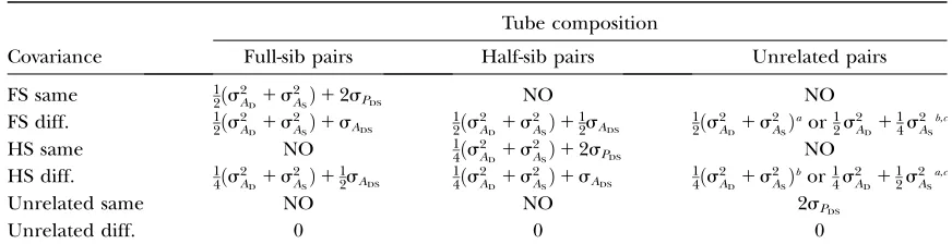
To investigate whether direct and associative genetic variances can be estimated from the data structure used in Wolf (2003), we derive general expressions for expectations of sire and dam covariances. We distin-guish between (i) covariances between individuals in the same group and (ii) covariances between individuals in different groups. The expected covariance between two individuals,iandj, in the same group is
CovðPi;PjÞ ¼rijðs2AD1s
2
ASÞ12sPDS ðA1Þ
and in different groups is
CovðPi; PjÞ ¼rijs2AD1ðri;mj1rj;miÞsADS1rmi;mjs 2
AS
ðA2Þ
in which rij is relatedness between i and j, ri;mj is re-latedness betweeniand the group member ofj,rj;mi is relatedness betweenjand the group member ofi, and
rmi;mjis relatedness between the group members ofiand
TABLE A1
Expectations of full- and half-sib covariances in the data structure used in WOLF(2003)
Tube composition
Covariance Full-sib pairs Half-sib pairs Unrelated pairs
FS same 1
2ðs2AD1s
2
ASÞ12sPDS NO NO
FS diff. 1
2ðs
2
AD1s
2
ASÞ1sADS
1 2ðs
2
AD1s
2
ASÞ1
1 2sADS
1 2ðs
2
AD1s
2
ASÞ
aor1 2s
2
AD1
1 4s
2
AS
b,c
HS same NO 1
4ðs
2
AD1s
2
ASÞ12sPDS NO
HS diff. 1
4ðs2AD1s
2
ASÞ1
1 2sADS
1 4ðs2AD1s
2
ASÞ1sADS
1 4ðs2AD1s
2
ASÞ
bor1 4s2AD1
1 2s2AS
a,c
Unrelated same NO NO 2sPDS
Unrelated diff. 0 0 0
FS, full sibs; HS, half sibs; same, in the same group; diff., in different groups; NO, this combination does not occur.
a
When the group members of both individuals are full sibs. b
When the group members of both individuals are half sibs. c
j. Table A1 shows expected covariances between full sibs, half sibs, and unrelated individuals for each of the three tube compositions used in Wolf (2003). The expecta-tions of sire and dam covariances given in Table 3 differ from those presented in Wolf (2003), primarily be-cause covariances due to group members of full and half sibs are incomplete in Wolf(2003).
It follows from Equations A1 and A2 thats2
ADands
2
AS
can be separated only when rij6¼rmi;mj. Thus the in-formation in the data to separates2
ADands
2
AS depends
on whether and how frequently rij 6¼rmi;mj occurs. It follows from Table A1 thatrij6¼rmi;mj occurs only in the situation where groups consist of two unrelated individ-uals and only when relatedness between the two group members of both individuals differs from that between both individuals considered. (see Table A1 footnote). Whether or not that situation occurs in the data depends on details of the experimental implementation that are not described in Wolf(2003). Thus, the data
structure used in Wolf(2003) provides either very little or no information at all to separate the direct and the associative heritable variance.
To validate this theoretical result we performed Monte Carlo simulation of the data structure used in Wolf(2003), where, in the case of groups consisting of unrelated individuals, group members of full sibs were full sibs as well, and group members of half sibs were half sibs as well. Hence, theoretically this data structure should not contain any information to separates2
ADand
s2
AS. Statistical analyses of the simulated data using
Equations 4 and 5 as a model showed that the matrix of second derivatives of the likelihood (Fisher’s in-formation matrix) was singular, indicating that there are an infinite number of combinations of parameters that yield the identical maximum likelihood. Indeed identical maximum likelihoods were observed for mul-tiple combinations ofs2
ADands
2
AS, which confirms the