Improved Confidence Intervals in Quantitative Trait Loci Mapping by
Permutation Bootstrapping
Jo
¨rn Bennewitz, Norbert Reinsch and Ernst Kalm
1Institut fu¨r Tierzucht und Tierhaltung, Christian-Albrechts-Universita¨t, D-24098 Kiel, Germany Manuscript received July 30, 2001
Accepted for publication January 9, 2002
ABSTRACT
The nonparametric bootstrap approach is known to be suitable for calculating central confidence intervals for the locations of quantitative trait loci (QTL). However, the distribution of the bootstrap QTL position estimates along the chromosome is peaked at the positions of the markers and is not tailed equally. This results in conservativeness and large width of the confidence intervals. In this study three modified methods are proposed to calculate nonparametric bootstrap confidence intervals for QTL loca-tions, which compute noncentral confidence intervals (uncorrected method I), correct for the impact of the markers (weighted method I), or both (weighted method II). Noncentral confidence intervals were computed with an analog of the highest posterior density method. The correction for the markers is based on the distribution of QTL estimates along the chromosome when the QTL is not linked with any marker, and it can be obtained with a permutation approach. In a simulation study the three methods were compared with the original bootstrap method. The results showed that it is useful, first, to compute noncentral confidence intervals and, second, to correct the bootstrap distribution of the QTL estimates for the impact of the markers. The weighted method II, combining these two properties, produced the shortest and less biased confidence intervals in a large number of simulated configurations.
S
EVERAL statistical methods were proposed for de- the endpoints of the confidence interval are calculated tecting quantitative trait loci (QTL) using marker by finding the locations at either side of the estimated information. Most of them are based either on maximum- QTL position having the maximum LOD score that likelihood procedures (Lander and Botstein 1989) have a LOD score of 1 unit less than the estimated QTL or on regression methods (Haley and Knott 1992; position. The confidence interval is then defined by allMartinezandCurnow1992). However, none of these those points on the chromosome where the LOD score
methods led to a straightforward calculation of a confi- has fallen within 1 unit from the maximum (i.e., the dence interval. These are intervals on the chromosomes positions between the two interval endpoints). However, that contain the QTL with a given coverage probability this method often produces intervals that are too short; P (usually 90 or 95%). Calculating small confidence i.e., the intervals contain the QTL with a lower coverage intervals that hold the stated coverage probability is of probability than stated.Van Ooijen(1992) andMangin
fundamental importance for practical breeding pur- et al. (1994) showed this to be the case for small and poses as well as for molecular biologists. For example, medium-sized populations and for QTL of small effects breeders who wish to use the marker information in because the regular conditions for the conversion of marker-assisted selection (MAS) breeding schemes the likelihood-ratio test toward a chi-square distribution need to know the optimum length of the chromosome do not hold in these genetic configurations. To attain segment of interest, and biologists need this knowledge a higher probability of containing the QTL,Van Ooijen
for any further decisions regarding experimental fine- (1992) suggested that the LOD drop-off confidence
in-mapping strategy. tervals should be based on two LOD differences. In
Different methods were described to calculate confi- a simulation study it was found that the sizes of these dence intervals in QTL mapping.Conneallyet al.(1985) confidence intervals were large and variable (Van Ooijen andLanderandBotstein (1989) proposed the LOD 1992) and, in population sizes used in real QTL mapping drop-off method. This is based on the conversion of procedures, unsatisfactory for QTL with smaller effects. the distribution of the likelihood-ratio test statistic of Mangin et al. (1994) and Mangin and Goffinet linkagevs.no linkage between a marker and a putative (1997) developed complex formulas for calculating con-QTL into a chi-square distribution. Using this method, fidence intervals. These are based on a maximum-likeli-hood-ratio test using statistics in which asymptotic distri-bution does not depend on the effect of the QTL. The 1Corresponding author:Institut fu¨ r Tierzucht und Tierhaltung,
Her-major difficulty of this method is the computation of
mann-Rodewald-Str. 6, D-24118 Kiel, Germany.
E-mail: [email protected] the correct threshold for the likelihood-ratio test for
was generated and contained 300 or 500 (N ⫽ 300, 500) which ManginandGoffinet(1997) proposed an
ap-progeny. For each individual a single 100-cM chromosome proximate analytical solution.
(L⫽100 cM) evenly spaced with markers every 20 cM (⌬ ⫽
Visscheret al.(1996) introduced a nonparametric boot- 20 cM) was simulated. For calculating the crossover probabili-strap resampling approach (Efron 1979; Efron and ties the Kosambi mapping function was used. Each chromo-some contained a single segregating diallelic QTL with a
posi-Tibshirani1993) to construct a confidence interval for
tion midway between two flanking markers (d⫽30, 50 cM), a QTL position. The evaluation of generated bootstrap
closer to one of the flanking markers (d⫽ 25, 55 cM), or samples provided a distribution of QTL position
esti-directly at a marker position (d⫽20, 60 cM). The effect of mates along the chromosome that forms the base for the QTL was expressed in units of the polygenic standard the confidence interval calculation. Within a simulation deviation, and to cover a wide range of effects it was varied between 0.1, 0.5, and 1.0 (a⫽0.1, 0.5, 1.0). Additional simula-study they compared the nonparametric bootstrap
tions were carried out to investigate the impact of a longer method with the LOD drop-off method. The
nonpara-chromosome (L ⫽140 and 180 cM,⌬ ⫽20 cM,N ⫽ 300, metric bootstrap procedure seemed a good alternative
500 witha⫽0.5 anddin the middle of the chromosome) and to the LOD drop-off for defining confidence intervals a higher marker density [⌬ ⫽10 cM and 10/5 cM (additional for QTL positions, but tended to be unsuitably large markers at 35, 45, 55, and 65 cM),L⫽100 cM,a⫽0.5 with N⫽300, 500, respectively]. To avoid any confounding effects when the QTL effect was small.
due to different detection power (Darvasi et al. 1993) the To reduce the width of the estimated bootstrap
con-QTL position was located exactly midway between two flanking fidence interval a selective nonparametric bootstrap
markers when marker spacing was reduced (d⫽55 cM when method was proposed by Lebreton and Visscher ⌬ ⫽10 cM andd⫽52.5 cM when⌬ ⫽10/5 cM).
(1998). Their selection was based on criteria related to The total genetic variance was the sum of the polygenic variance and the variance due to the QTL. The polygenic the assumed genetic model. By comparing both
meth-genetic component was normally distributed. The heritability ods in a simulation study they found that the selective
of the trait, defined as the polygenic variance divided by the bootstrap method produced smaller confidence
inter-sum of polygenic variance and the nongenetic variance, was vals with a reduced conservativeness. Moreover, they assumed to be 0.25. Random nongenetic factors were normally showed that there is scope for improvement of the classi- distributed. For each simulated genetic configuration 1000 replicates were generated. The simulation program was writ-cal bootstrap approach for writ-calculating confidence
inter-ten in FORTRAN 77, supplemented with routines from the vals as proposed byVisscheret al.(1996).
NAG library (Numerical Algorithms Group1990). QTL
Wallinget al.(1998) provided a parametric bootstrap
analyses were done by using the programs BIGMAP and resimulation method (Efron1982) as an alternative to ADRQLT (briefly described inReinsch1999) and were based the nonparametric bootstrap approach and tested this on the multimarker regression described by Knott et al. (1994). Confidence intervals were calculated with FORTRAN method in a simulation study. As the authors themselves
77 programs and SAS procedures (SAS Institute1992). pointed out, the parametric bootstrap method produced
Generating the bootstrap samples:A total of 250 nonpara-poor results: The derived confidence intervals varied
metric bootstrap samples for each genetic configuration were from conservative intervals when the QTL position was generated as described byVisscheret al.(1996). Briefly, for at the location of the marker to anticonservative inter- each single bootstrap sampleN observations out of the pool ofNoriginal observations were drawn with replacement, so vals when the QTL position was between two markers.
that each observation consisted of an individual’s marker ge-A main result from the study ofWallinget al.(1998)
notype and the corresponding phenotype. Some observations was the discovery of a bias in calculating confidence
may appear more than one time in a bootstrap sample while intervals from the distribution of QTL position estimates others may be not included at all. Each single bootstrap sample from nonparametric bootstrap samples. This bias is de- was analyzed and the best estimate of the position of the QTL was recorded. After 250 bootstrap samples the distribution of fined as a significant difference between the observed
the 250 estimates of the QTL position was derived by ordering and the stated coverage probability and is deemed to
them along the chromosome. Because the QTL is linked to have been caused by the locations of the markers. Elimi- two flanking markers, this distribution is termed thelinkage nating this bias would probably result in smaller confi- distribution.
dence intervals. As mentioned byLebretonandVisscher Modeling marker impact on bootstrap distributions:As re-ported byWallinget al.(1998) the reasons for the marker (1998), an additional reduction of the interval width could
impact on the distribution of the bootstrap estimates for the be possible by computing noncentral confidence intervals.
QTL position are an accumulation of the type I error rate at Taking this into consideration, we present three modified the marker loci and the general trend of the mapping proce-nonparametric bootstrap schemes to calculate confidence dure to put the estimate of a QTL position toward a marker locus. In the following section a closer look at this marker intervals: (i) noncentral, (ii) marker corrected, and (iii)
impact is presented by a simple model, and the theoretical noncentral and marker corrected. Within a simulation
background for a marker correction is given. At first we focus study these schemes were compared with the
nonparamet-on the expected distributinonparamet-on of the best estimates for a QTL ric bootstrap method presented byVisscheret al.(1996). position out of a bootstrap sample when a QTL may be present but not linked with any marker. This distribution is termed thenull distribution, because every estimate indicates a type I MATERIALS AND METHODS error. In this null distribution the probability of each position
achieving the best estimate would be Simulation: A first generation backcross population
whereP(i)ndis the probability of obtaining the best estimate one-half of the given error rate of 1⫺Pwas subtracted from
each side of the corrected distribution during the computation for position i on the chromosome in the null distribution
(nd),Peis the probability for each position achieving the best of the confidence intervals, in the weighted method II an
analog highest posterior density (HPD) method was used to estimate assuming equal probabilities for each position, and
S(i) is a “selection coefficient” of positioniin the null distribu- obtain noncentral intervals when the corrected distribution is not tailed equally. This method was adapted from the standard tion. BecausePeis a constant with the same value for every
position (i.e., one divided through the number of possible HPD approach as described inBoxandTiao(1992) and is presented in detail in theappendix.
QTL positions), it can be stated
Uncorrected method I:This method was the original one P(i)nd⬀S(i). (2) as proposed by Visscheret al. (1996) and did not correct for the marker impact. The central confidence intervals were The selection coefficient describes the probability of each
calculated directly from the linkage distribution by taking position to obtain the best estimate as a deviation from the
the top and bottom 2.5th and 5th percentiles of the linkage equal distribution and is determined by the position and the
distribution as the upper and lower interval endpoints, respec-informativeness of the marker loci. It would be highest at the
tively. marker loci and lower at the loci between the markers. In this
Uncorrected method II:In this method confidence intervals model, it is assumed that the selection coefficientS(i) is the
were computed from the linkage distribution with the analog same for both the linkage distribution and the null
distribu-HPD method described in theappendix.The calculated inter-tion. The probability of each position in the linkage
distribu-vals were noncentral and not marker corrected. tion [P(i)ld] to obtain the best estimate would be
The confidence intervals with the stated coverage probabil-ityPof 95 and 90% were calculated for each replicate by the P(i)ld⬀P(i)*QTLS(i), (3)
four methods described above, and it was assessed whether whereP(i)QTLis the probability of each positioniachieving the QTL was located within these intervals or not. The rate
the best estimate when a QTL is linked with a marker and is, of the confidence intervals for each simulated genetic config-of course, influenced by the effect config-of the QTL but not by uration that did not include the simulated position of the the markers per se. Following Equation 3, an approximate QTL was termed thenoninclusion rate(NI), and this should correction for the impact of the markers can be achieved by be not greater than 1⫺P.For each configuration the aver-weighting the probability of each position from the linkage age width of the confidence interval out of 1000 replicates distribution with the reciprocal value of the corresponding was also calculated, and this is ideally small.
selection coefficient:
P(i)QTL⬀P(i)ld/S(i). (4)
RESULTS The distribution resulting from the corrected probabilities
[P(i)QTL] to attain the best estimate for the QTL location is The initial results for all four bootstrap schemes are
termed thecorrected distribution. presented in Tables 1–4. Summarized over all genetic Weighted method I:In the weighted method the marker configurations analyzed, the uncorrected method I pro-correction approach was followed. First, the probability in the
duced the largest and most conservative confidence in-linkage distribution to attain the best estimateP(i)ldand the
tervals. A reduction of the interval width and conserva-selection coefficientS(i) had to be determined for each
posi-tion on the chromosome. The values forP(i)ldwere the corre- tiveness was possible using the uncorrected method II.
sponding observed frequencies of best QTL estimates in the Further reduction of the width was achieved using the linkage distribution [f(i)ld]:
weighted method I and, even more, by the weighted method II without lifting the noninclusion rate seriously P(i)ld⫽f(i)ld. (5)
above 1⫺P. The linkage distribution was obtained as described above. The
QTL effect: As expected, an increase of the QTL selection coefficientsS(i) were calculated by computing the
effect resulted in a smaller confidence interval for all null distribution for each simulated genetic configuration.
This was achieved by setting the recombination rate between bootstrap schemes (Table 1 and 2). It is very unlikely the simulated QTL and every marker locus to 0.5. The null that a QTL with an effect ofa ⫽0.1 (this QTL would distribution was then built by the best estimates out of all
explain only 0.13% of the total variance in our simulated bootstrap samples and all replicates (250 estimates⫻ 1000
populations) would be detected in real mapping experi-replicates) for each simulated genetic configuration.
Follow-ments and, hence, the uncorrected method I produced ing Equation 2 the selection coefficient for each position on
the chromosome was the corresponding frequency of the best very conservative confidence intervals, which cover almost estimates in the null distribution [f(i)nd]: the whole chromosome. For this low QTL effect each
confidence interval produced by this method was⬎93 cM. S(i)⫽ f(i)nd. (6)
However, the uncorrected method II (weighted method I, For each replicate the distribution of the probabilitiesP(i)QTL weighted method II) produced 90% intervals for this
(the corrected distribution) was calculated using (4).
small QTL effect that were significantly⬍90 cM (85 cM, The confidence intervals with a coverage probabilityPof
80 cM) for the 90% confidence intervals and were less 95 and 90% were calculated by using the top and the bottom
2.5th and 5th percentiles as the upper and lower interval conservative. All confidence intervals for situations of endpoints, respectively. The obtained confidence intervals a⫽0.1 were only marginally influenced by the remain-were central.
ing genetic parameters. Weighted method II:For the weighted method II the
cor-Elevating the QTL effect from a ⫽ 0.1 to 0.5 (this rected distribution was computed in the same manner as for
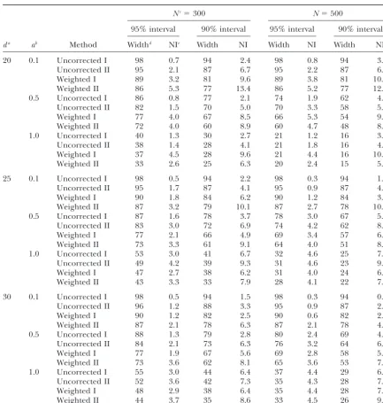
TABLE 1
Effect of QTL position within marker interval, population size, and QTL effect on the confidence intervals for the different bootstrap methods—QTL position proximal
Nc⫽300 N⫽500
95% interval 90% interval 95% interval 90% interval
da ab Method Widthd NIe Width NI Width NI Width NI
20 0.1 Uncorrected I 98 0.7 94 2.4 98 0.8 94 3.2
Uncorrected II 95 2.1 87 6.7 95 2.2 87 6.9
Weighted I 89 3.2 81 9.6 89 3.8 81 10.9
Weighted II 86 5.3 77 13.4 86 5.2 77 12.6
0.5 Uncorrected I 86 0.8 77 2.1 74 1.9 62 4.2
Uncorrected II 82 1.5 70 5.0 70 3.3 58 5.6
Weighted I 77 4.0 67 8.5 66 5.3 54 9.9
Weighted II 72 4.0 60 8.9 60 4.7 48 8.0
1.0 Uncorrected I 40 1.3 30 2.7 21 1.2 16 3.2
Uncorrected II 38 1.4 28 4.1 21 1.8 16 4.1
Weighted I 37 4.5 28 9.6 21 4.4 16 10.0
Weighted II 33 2.6 25 6.3 20 2.4 15 5.7
25 0.1 Uncorrected I 98 0.5 94 2.2 98 0.3 94 1.3
Uncorrected II 95 1.7 87 4.1 95 0.9 87 4.0
Weighted I 90 1.8 84 6.2 90 1.2 84 3.9
Weighted II 87 3.2 79 10.1 87 2.7 78 10.1
0.5 Uncorrected I 87 1.6 78 3.7 78 3.0 67 5.3
Uncorrected II 83 3.0 72 6.9 74 4.2 62 8.5
Weighted I 77 2.1 66 4.9 69 3.4 57 6.0
Weighted II 73 3.3 61 9.1 64 4.0 51 8.2
1.0 Uncorrected I 53 3.0 41 6.7 32 4.6 25 7.1
Uncorrected II 49 4.2 39 9.3 31 4.6 23 9.5
Weighted I 47 2.7 38 6.2 31 4.0 24 6.1
Weighted II 43 3.3 33 7.9 28 4.1 22 7.6
30 0.1 Uncorrected I 98 0.5 94 1.5 98 0.3 94 0.9
Uncorrected II 96 1.2 88 3.3 95 0.9 87 2.5
Weighted I 90 1.2 82 2.5 90 0.6 82 2.5
Weighted II 87 2.1 78 6.3 87 2.1 78 4.8
0.5 Uncorrected I 88 1.3 79 2.8 80 2.4 69 4.5
Uncorrected II 84 2.1 73 6.3 76 3.2 64 6.4
Weighted I 77 1.9 67 5.6 69 2.8 58 5.1
Weighted II 73 3.6 62 8.1 65 3.6 53 7.3
1.0 Uncorrected I 55 3.0 44 6.4 37 4.4 29 6.7
Uncorrected II 52 3.6 42 7.3 35 4.3 28 7.9
Weighted I 48 2.9 38 6.4 35 4.4 28 7.1
Weighted II 44 3.7 35 8.6 33 4.5 26 9.0
Data were simulated with a 100-cM chromosome and a marker spacing of 20 cM. The number of bootstrap samples was 250 and the number of replicates for each genetic configuration was 1000.
aPosition of the simulated QTL (in centimorgans from the start of the chromosome). bQTL effect, expressed in units of the polygenic standard deviation.
cPopulation size.
dAverage width (in centimorgans) of the confidence interval.
eNoninclusion rate, the rate of the confidence intervals that do not contain the real QTL position.
the average 90% interval width by 15–25 cM. The respec- bootstrap schemes. The reduction for the 90% confi-dence intervals varied between 2 and 4 cM. The corre-tive change by stepping 0.5 to 1.0 (11.8% of the total
variance) was 40–50 cM, depending on the population sponding changes were between 1 and 5 cM when marker distance was reduced to 10 cM and when addi-size and QTL position. This reduction was remarkably
constant for the four methods. tional markers were added around the QTL position, depending on the population size and the bootstrap
Marker spacing:Changing marker distances from 20
to 10 cM (top of Table 2 and Table 3) and adding four scheme. No general dependency of the noninclusion rate on the marker density was observed for any method. additional markers around the QTL position (Table
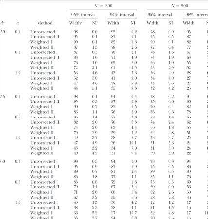
TABLE 2
Effect of QTL position within marker interval, population size, and QTL effect on the confidence intervals for the different bootstrap methods—QTL position central
Nc⫽300 N⫽500
95% interval 90% interval 95% interval 90% interval
da ab Method Widthd NIe Width NI Width NI Width NI
50 0.1 Uncorrected I 98 0.0 95 0.2 98 0.0 95 0.6
Uncorrected II 95 0.1 87 1.1 95 0.5 87 1.4
Weighted I 90 0.1 82 1.3 90 0.1 82 0.7
Weighted II 87 1.3 78 2.6 87 0.4 77 2.0
0.5 Uncorrected I 87 0.5 78 2.1 78 1.6 67 3.6
Uncorrected II 83 1.6 71 4.9 74 1.9 63 7.1
Weighted I 76 1.0 65 2.9 66 1.9 55 4.6
Weighted II 72 2.1 61 5.5 63 2.9 52 7.7
1.0 Uncorrected I 53 4.6 43 7.3 36 2.9 28 6.9
Uncorrected II 52 5.0 41 9.0 34 4.0 27 7.1
Weighted I 47 4.6 38 7.3 34 2.6 27 6.5
Weighted II 44 5.1 35 8.3 32 4.2 25 8.2
55 0.1 Uncorrected I 98 0.1 94 0.4 98 0.2 94 0.7
Uncorrected II 95 0.3 87 1.9 95 0.6 86 2.5
Weighted I 90 0.2 82 1.5 90 0.4 82 0.7
Weighted II 86 1.1 76 2.9 86 0.6 78 3.3
0.5 Uncorrected I 86 1.4 77 3.3 78 1.4 66 3.7
Uncorrected II 82 2.0 70 6.3 74 2.4 62 6.2
Weighted I 74 2.0 63 4.4 66 1.8 55 4.1
Weighted II 70 2.9 59 7.2 62 2.8 51 7.0
1.0 Uncorrected I 49 3.7 38 7.7 33 3.7 25 8.1
Uncorrected II 47 4.9 36 10.1 31 5.3 24 9.2
Weighted I 43 3.2 34 7.0 31 3.0 24 6.8
Weighted II 40 4.2 31 9.4 29 3.9 22 7.8
60 0.1 Uncorrected I 98 0.3 94 1.0 98 0.3 94 1.0
Uncorrected II 95 0.9 87 1.9 95 0.5 86 2.1
Weighted I 89 0.7 81 2.4 89 0.5 80 1.7
Weighted II 86 1.8 77 4.1 85 1.1 76 4.1
0.5 Uncorrected I 83 0.8 72 1.6 73 0.5 60 1.8
Uncorrected II 79 1.4 67 3.4 69 0.9 56 3.8
Weighted I 71 2.0 60 5.4 62 2.6 50 7.7
Weighted II 67 3.2 55 6.6 58 2.8 46 7.3
1.0 Uncorrected I 40 1.5 30 4.2 22 1.2 17 2.2
Uncorrected II 38 2.3 28 4.1 21 1.5 16 3.0
Weighted I 36 5.2 27 10.7 22 4.8 17 10.2
Weighted II 33 3.7 24 6.8 20 2.5 15 4.8
Data were simulated with a 100-cM chromosome and a marker spacing of 20 cM. The number of bootstrap samples was 250 and the number of replicates for each genetic configuration was 1000.
aPosition of the simulated QTL (in centimorgans from the start of the chromosome). bQTL effect, expressed in units of the polygenic standard deviation.
cPopulation size.
dAverage width (in centimorgans) of the confidence interval.
eNoninclusion rate, the rate of the confidence intervals that do not contain the real QTL position.
of the population size fromN⫽300 toN⫽500 led to quently there was the most space for reduction. It was not possible to assign a change of noninclusion rates significantly smaller confidence intervals for all four
bootstrap schemes. This reduction was only marginal to the effect of an increased population size for the uncorrected method II and for the weighted methods fora ⫽ 0.1 but for a ⫽ 0.5 it was between 12 and 14
cM and fora ⫽1.0 it was between 10 and 15 cM. The I and II; it appears that the intervals computed with the uncorrected method I were in general less conservative uncorrected method I was most sensitive for increased
population size as the reduction of the interval width when the population size was increased.
In general, a gain of information, provided by a greater was greatest. This might be due to the fact that intervals
TABLE 3
Effect of an increased marker density on the confidence intervals for the different bootstrap methods
Nc⫽300 N⫽500
95% interval 90% interval 95% interval 90% interval
⌬a db Method Widthd NIe Width NI Width NI Width NI
10 55 Uncorrected I 84 0.5 74 2.7 76 2.1 64 3.6
Uncorrected II 79 1.6 68 5.5 71 3.0 59 7.7
Weighted I 73 1.5 61 4.1 64 2.0 53 5.9
Weighted II 68 3.0 57 6.1 61 3.8 49 8.1
10/5 52.5 Uncorrected I 82 1.1 71 3.2 70 0.4 59 2.3
Uncorrected II 77 1.8 64 5.6 67 1.5 54 5.2
Weighted I 72 1.2 61 3.8 62 1.2 50 4.2
Weighted II 68 2.6 56 6.8 58 2.7 47 6.6
Data were simulated with a 100-cM chromosome and a simulated QTL effect ofa⫽0.5 units of the polygenic standard deviation. The number of bootstrap samples was 250 and the number of replicates for each genetic configuration was 1000.
aMarker spacing (10 ⫽one marker every 10 cM, 10/5⫽four additional markers every 5 cM around the
simulated QTL position).
bPosition of the simulated QTL (in centimorgans from the start of the chromosome). cPopulation size.
dAverage width (in centimorgans) of the confidence interval.
eNoninclusion rate, the rate of the confidence intervals that do not contain the real QTL position.
consistent with other studies concerning QTL bootstrap for all bootstrap schemes;i.e., the increase of the chro-mosome length resulted in larger intervals and, in most confidence intervals (Visscher et al. 1996; Lebreton
andVisscher1998;Wallinget al.1998). The effect of cases, in slightly lower noninclusion rates (Table 4). The absolute difference between the length of the intervals the larger population size was stronger than the effect
of the higher marker density. produced by the four methods increased slightly with a longer chromosome without changing the ranking
Length of chromosome: The length of the
chromo-some had a large impact on the size of the confidence order.
QTL position:The effect of the QTL position can be intervals and a small impact on the noninclusion rates
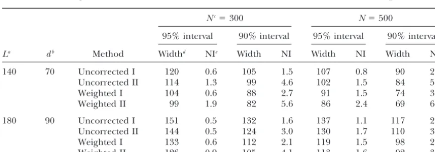
TABLE 4
Effect of the length of the chromosome on the confidence intervals for the different boostrap methods
Nc⫽300 N⫽500
95% interval 90% interval 95% interval 90% interval
La db Method Widthd NIe Width NI Width NI Width NI
140 70 Uncorrected I 120 0.6 105 1.5 107 0.8 90 2.3
Uncorrected II 114 1.3 99 4.6 102 1.5 84 5.4
Weighted I 104 0.6 88 2.7 91 1.5 74 3.9
Weighted II 99 1.9 82 5.6 86 2.4 69 6.2
180 90 Uncorrected I 151 0.5 132 1.6 137 1.1 117 2.8
Uncorrected II 144 0.5 124 3.0 130 1.7 110 3.6
Weighted I 133 0.6 112 2.1 119 1.5 98 2.6
Weighted II 126 0.9 105 4.1 113 1.6 92 3.0
Data were simulated with a marker spacing of 20 cM and a simulated QTL effect of a⫽0.5 units of the polygenic standard deviation. The number of bootstrap samples was 250 and the number of replicates for each genetic configuration was 1000.
aChromosome length (in centimorgans).
bPosition of the simulated QTL (in centimorgans from the start of the chromosome). cPopulation size.
dAverage width (in centimorgans) of the confidence interval.
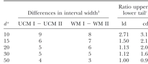
TABLE 5 attributed to two factors: the QTL position within a
marker interval (midway between two markers, closer Effect of the QTL position on the differences between the to one marker, or at the same position as the marker) widths of central and noncentral confidence intervals and the chromosomal QTL position, whether proximal
or central. To avoid any confounding effects these two Ratio upper/
Differences in interval widthb lower tailc
factors were analyzed separately.
It seems that when the QTL is located centrally (posi- da UCM I⫺UCM II WM I⫺WM II ld cd
tion 60 instead of 20, 55 instead of 25, and 50 instead of
10 9 8 2.71 3.18
30; Tables 1 and 2) the computed intervals are smaller,
15 6 7 1.50 2.18
regardless of the method. This is in close agreement
20 5 6 1.13 2.07
withLebretonandVisscher(1998) andWallinget al. 30 5 5 1.12 1.60
(1998) and may be caused by the fact that the mapping 50 4 3 1.00 0.98 procedure tends to estimate the QTL position closer to
Data were simulated with a 100-cM chromosome, a marker the middle of the chromosome, as reported by Hyne
spacing of 20 cM, and a simulated QTL effect ofa⫽0.5 units et al.(1995). Additionally, the noninclusion rates were
of the polygenic standard deviation. The population size was in general lower fora⫽0.1 anda⫽0.5 but higher for 500. The number of bootstrap samples was 250 and the num-a⫽1.0 for all methods. ber of replicates for each genetic configuration was 1000.
aPosition of the simulated QTL (in centimorgans from the
Changing the QTL position within the marker
inter-start of the chromosome). val from midway between two flanking markers toward
bAverage differences of the 90% interval width computed
a marker position (top, middle, and bottom of Tables
by the uncorrected methods I and II (UCM I⫺UCM II) and 1 and 2) resulted in significantly smaller confidence by the weighted methods I and II (WM I⫺WM II). intervals for all four methods. For example, the reduc- cRatio of subtracted upper tail and subtracted lower tail
from linkage distribution (ld) and the corrected distribution tion for the 90% interval fora⫽0.5 andN⫽500 was
(cd) during computation of the 90% confidence interval by between 1 and 2 cM whend was changed from 50 to
the analog HPD method. 55 cM and ⵑ4 cM when d was changed from 55 to
60 cM, regardless of the method. The uncorrected meth-ods I and II produced intervals that were more
conserva-tracted upper and lower tail from the distributions in-tive when the QTL and the marker positions are
identi-creased when the QTL was located closer to the start cal compared to situations with QTL positions midway
of the chromosome (Table 5). The increase of the ratio between two flanking markers. This is consistent with
was greater for the intervals computed from the cor-the findings ofWallinget al.(1998). The noninclusions
rected distribution than for those computed from the were in general increased for the weighted method I when
linkage distribution. When the QTL was midway on the dwas moved toward a marker position whereas no general
chromosome (d⫽50 cM) the ratio became, as expected, dependency could be observed between the QTL position
exactly one or near to one. It is important to note that and the noninclusion rates for the weighted method II.
the computed intervals for d ⫽ 10 cM were slightly Another remarkable topic might be the differences
anticonservative (10.4, 12.5, 12.9, and 13.9% noninclu-between the interval widths from the uncorrected
meth-sions for the 90% intervals computed with uncorrected ods I and II on the one hand and the differences
be-methods I and II and the weighted be-methods I and II, tween the weighted methods I and II on the other hand
respectively; results not shown). when moving the QTL closer to the start of the
chromo-Selection step:In practical QTL mapping experiments some. To investigate the impact of the QTL position on
confidence intervals would be computed only when the these differences in detail, additional simulations with
QTL is declared significant. To investigate whether the N⫽500,a⫽0.5,⌬ ⫽20 cM,L⫽100 cM, and a QTL
rejection of nonsignificant replicates would change the position at d ⫽ 10 or 15 cM were carried out. The
results a selection step for two genetic configurations average 90% interval widths computed with the
uncor-similar toVisscheret al.(1996) was introduced. First, rected method II (weighted method II) were subtracted
according toChurchillandDoerge(1994), threshold from the corresponding intervals computed with the
levels that gave a nominal type I error rate of 10 and 5% uncorrected method I (weighted method I) for the
ge-were calculated by taking the 90th and 95th quantiles of netic configurations described above and the same
con-the test statistic of 10,000 analyzed simulated populations figurations but withd⫽20 and 30 cM (Table 1) andd⫽
with no segregating QTL. Confidence intervals were com-50 cM (Table 2). Additionally, the ratio of the subtracted
puted only for replicates that showed QTL test statistics upper tail and the subtracted lower tail of the linkage
above the threshold. The results show that all computed distribution and the corrected distribution during the
confidence intervals were smaller and less conservative computation of the 90% confidence interval with the
when introducing a selection step (top of Table 2 and analog HPD method were calculated. The results show
Table 6) and when reducing the nominal type I error rate that both the differences between the central and
TABLE 6
Effect of rejection of nonsignificant replicates on the confidence intervals for the different bootstrap methods
Nb⫽300 N⫽500
95% interval 90% interval 95% interval 90% interval
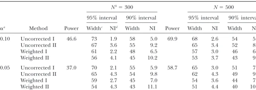
␣a Method Power Widthc NId Width NI Power Width NI Width NI
0.10 Uncorrected I 46.6 73 1.9 58 5.0 69.9 68 2.6 54 5.3
Uncorrected II 67 3.6 55 9.2 65 3.4 52 8.7
Weighted I 61 2.2 48 6.5 57 3.0 46 6.7
Weighted II 56 4.1 45 10.2 53 3.7 43 9.5
0.05 Uncorrected I 37.0 70 2.1 55 5.9 58.7 65 3.0 51 7.2
Uncorrected II 65 4.3 54 9.8 62 4.3 49 9.9
Weighted I 59 2.7 45 7.0 54 3.6 44 7.8
Weighted II 54 4.3 43 11.1 51 4.4 40 10.7
Data were simulated with a marker spacing of 20 cM and a simulated QTL effect of a⫽0.5 units of the polygenic standard deviation. The QTL position was at 50 cM. Confidence intervals were computed only when the population showed a significant QTL. Experimental power was defined as the percentage of replicates that show a test statistic above threshold value corresponding to the nominal type I error rate. The number of bootstrap samples was 250 and the number of replicates for each genetic configuration was 1000.
aNominal type I error rate. bPopulation size.
cAverage width (in centimorgans) of the confidence interval.
dNoninclusion rate, the rate of the confidence intervals that do not contain the real QTL position.
al.(1996). Generally, the change of the nominal error al.2000). However, this method produces intervals that tend to be rather large and conservative, and therefore rate from 10 to 5% reduced the interval width between
1 and 3 cM and increased the noninclusion rate by we proposed three methods (uncorrected method II and weighted methods I and II) to improve this classical
ap-ⵑ1–2%. No differences in sensitivity for the selection
step between the four bootstrap methods could be ob- proach to calculate smaller and less conservative confi-dence intervals and compared these methods within a served.
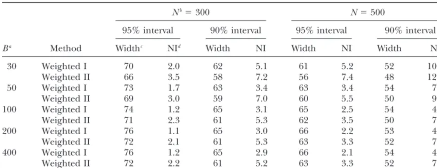
Number of bootstrap samples: In computing confi- simulation study with the classical approach.
Bias of confidence intervals:The bias of confidence dence intervals from the linkage distributionVisscher
et al.(1996) showed that there is only a small impact on intervals for QTL position estimates (biasci) can be
de-fined as the number of bootstrap samples. To examine whether
this holds also for the computation of intervals from the
biasci⫽ NI⫺ (1⫺P),
corrected distribution, the number of bootstrap samples
was varied for two genetic configurations (⌬ ⫽20 cM, where NI is the noninclusion rate. The biasci for the a⫽0.5,L⫽100,d⫽50 cM, andN⫽300, 500, respec- intervals computed with the uncorrected method I was tively). It seems that there is a lower bound for the number in general greatest and was upward except when the of bootstrap samples to generate the corrected distribu- QTL was at the start of the chromosome and signifi-tion for interval computasignifi-tion that is between 100 and cantly increased for this method when the QTL position 200 and dropping it below 100 results in smaller intervals was located at a marker position. This is in agreement with a higher noninclusion rate. Increasing the number with the findings ofVisscheret al.(1996) andWalling
of bootstrap samples above 200 did not change the results et al.(1998). When comparing the uncorrected method (Table 7). Following this, the number of bootstrap sam- I with the weighted method I and the uncorrected ples (250) used in this study is appropriate. method II with the weighted method II, respectively, it follows that the marker correction of the linkage distri-bution leads in general to a reduced bias of the confi-DISCUSSION
dence intervals as the noninclusion rate becomes closer to 1⫺P.Note that this bias was for the weighted method The classical bootstrap method (in this study the
un-corrected method I) for calculating confidence intervals I, and even more, for the weighted method II, slightly downward, but not substantial, when the QTL effect for a QTL position as proposed byVisscheret al.(1996)
seems a suitable and practical approach, and in some was small and the QTL was located at the start of the chromosome but upward for the remaining configura-recent real QTL mapping projects this method was used
to obtain confidence intervals for the QTL position (e.g., tions. Together with the fact that the weighted methods I and II produced significantly smaller confidence
TABLE 7
Effect of number of bootstrap samples on the confidence intervals for the weighted methods I and II
Nb⫽300 N⫽500
95% interval 90% interval 95% interval 90% interval
Ba Method Widthc NId Width NI Width NI Width NI
30 Weighted I 70 2.0 62 5.1 61 5.2 52 10.1
Weighted II 66 3.5 58 7.2 56 7.4 48 12.7
50 Weighted I 73 1.7 63 3.4 63 3.4 54 7.2
Weighted II 69 3.0 59 7.0 60 5.5 50 9.8
100 Weighted I 74 1.2 65 3.1 65 2.5 54 4.9
Weighted II 71 2.3 61 5.3 62 3.5 50 7.8
200 Weighted I 76 1.1 65 3.0 66 2.2 53 4.6
Weighted II 72 2.1 61 5.3 63 3.3 52 7.6
400 Weighted I 76 1.2 65 2.9 66 2.1 54 4.5
Weighted II 72 2.2 61 5.2 63 3.3 52 7.8
Data were simulated with a marker spacing of 20 cM and a simulated QTL effect ofa⫽0.5 units of the polygenic standard deviation. The number of replicates for each genetic configuration was 1000.
aNumber of bootstrap samples. bPopulation size.
cAverage width (in centimorgans) of the confidence interval.
dNoninclusion rate, the rate of the confidence intervals that do not contain the real QTL position.
vals than the uncorrected methods I and II it follows an increased marker density (10 cM) 64% of the esti-mates would be placed at the marker loci. Except for that the described model of characterizing the marker
impact (Equations 1–4) and the marker correction in the marker density and chromosome length it seems that the null distribution is of little variability, since the weighted methods I and II is appropriate to obtain
smaller and less biased bootstrap confidence intervals varying the QTL effect and the population size resulted in almost the same null distribution (not shown). for the location of QTL that appear to be significant.
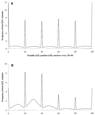
Note that the probability of making a type I error is a The extent of the influence of the markers on the linkage distribution depends on the level of the QTL function of the chosen significance level, which is not
affected by any of the presented methods to compute effect as it is shown in (3). Figure 1B shows an average linkage distribution from all bootstrap samples and all confidence intervals.
Marker correction: Although it may be possible to replicates forN ⫽500, L⫽ 100 cM,⌬ ⫽ 20 cM,a ⫽ 0.5, and for QTL position ofd ⫽30 cM from the start calculate the influence of the markers on the linkage
distribution, in terms of the selection coefficient for of the chromosome. When the QTL effect wasa⫽0.1 (a⫽0.5,a⫽1.0), 53% (32%, 9%) of the best estimates each possible QTL position (each centimorgan in our
study), in an analytical way, in this study it was done were located at the marker loci. The same genetic con-figurations but with a marker density of 10 cM gave empirically by computing the null distribution for each
genetic configuration,i.e., the distribution of the best roughly 10% higher values for the hits per marker locus, regardless of the QTL effect (results not shown), and QTL position estimates when there is no cosegregation
between the QTL and any marker, and, hence, every this confirmed the presence of the marker influence on the linkage distribution as first reported byWalling
estimate indicates a type I error per definition. This was
possible because in the model it is assumed that the et al.(1998). The two higher peaks at 20 and 40 cM are a result of the high value of the product of PQTL and
selection coefficient is the same for the linkage
distribu-tion as for the null distribudistribu-tion. The selecdistribu-tion coefficient selection coefficients at these positions (Equation 3). Both are relatively high because the distance to the for each position was the corresponding frequency of
the best estimate in the null distribution (Equation 6). position with the simulated QTL is only 10 cM and a marker is located at these positions, respectively. It fol-In Figure 1A a null distribution for population size of
N⫽ 500, marker space of 20 cM, chromosome length lows from this and from the empirical results of the simulation (Tables 1 and 2) that the smaller the QTL ofL⫽100 cM, and QTL effect ofa⫽0.5 is presented.
When the QTL is not linked with any marker, the proba- effect (which is unknowna prioriin real mapping experi-ments) and the lower the population size the more bility for each position on the chromosome to achieve
the best estimate is significantly higher at the marker advisable it is to correct for the marker impact expressed in selection coefficients.
loci. Over 45% of the estimates were placed there
Figure1.—Distributions of bootstrap QTL esti-mates along the simulated chromosome. (A) Em-pirical distribution of the QTL estimates when the recombination rate between the QTL and every marker was set to 0.5 (null distribution). (B) Empirical distribution of the QTL estimates when the QTL position was put atd ⫽ 30 cM (linkage distribution). (C) Empirical distribution of the marker-corrected QTL estimates when the QTL position was put atd⫽30 cM (corrected distribution). (D) Empirical distribution of the QTL estimates when the QTL position was put at d⫽20 cM (linkage distribution). (E) Empirical distribution of the marker-corrected QTL esti-mates when the QTL position was put atd⫽20 cM (corrected distribution). A half-sib backcross family consisting ofN⫽500 individuals was simu-lated. The QTL effect wasa⫽0.5 and the markers were put at 0, 20, 40, 60, 80, and 100 cM, respec-tively. Data are from all bootstrap samples and all replicates (250⫻1000 estimates).
the frequency of the best estimate in the linkage distri- with the uncorrected methods I and II. Correcting this average distribution results in Figure 1E. Right from bution by the value of the corresponding selection
coef-ficient (see Equation 4) whereby the number of boot- position 60 cM the frequency of best estimates in this distribution became again nearly equal for all positions. strap samples should be⬎200 to compute a corrected
distribution suitable for calculating confidence intervals Most of the probability mass is put between the markers at the start of the chromosome and position 40, but at (Table 7). Figure 1C shows an average corrected
distri-bution again from all bootstrap samples and all repli- the marker coinciding with the QTL position (20 cM) the frequency is significantly reduced (ⵑ1%). Similar cates forN⫽500,⌬ ⫽20 cM,L⫽100 cM,d⫽30 cM,
anda⫽0.5. The peaks at the marker loci observed in patterns were observed at the positions of the markers flanking the QTL in the average corrected distribution Figure 1, A and B, disappeared and the highest
fre-quency of the best estimate was in the interval of the in Figure 1C (QTL midway between flanking markers). Note that for this genetic configuration the null distribu-markers flanking the QTL. Right from position 60 cM
the frequency became nearly equal for all positions (in- tion follows the distribution presented in Figure 1A rather well and is therefore not shown.
cluding marker positions).
An average linkage distribution for a situation QTL Computing the null distribution:In the simulation the null distributions were derived in a simplified manner by located at a marker position (d⫽20 cM) is presented
in Figure 1D (N⫽500,⌬ ⫽20 cM,L⫽100 cM,a⫽0.5). setting the recombination rate between the QTL and any marker to 0.5. This had the advantage that the The high peak at the QTL position can be attributed to
the relatively high values of PQTL and to the selection required CPU time was minimal, but is not possible
in real QTL mapping experiments. Alternatively, the coefficient at this point. In contrast to Figure 1B, the
accumulation of the effect of a highPQTLvalue and a high permutation approach as proposed byChurchilland Doerge(1994) can be used to compute the null distri-selection coefficient is focused only on one position (20
Figure1.—Continued.
tailored to the experiment. By repeatedly randomly position on the chromosome as described in our model, and so this distribution should be a very similar null shuffling the trait values while keeping the marker data
constant, they uncoupled the phenotype-genotype asso- distribution as obtained in this simulation. To show that the permutation method is suitable to calculate the null ciation, and after applying the QTL-mapping
proce-dure, every estimate would indicate a type I error per distribution we performed a further simulation with 1000 permutations of the phenotypic data for every replicate. definition. There is no reason why this distribution of
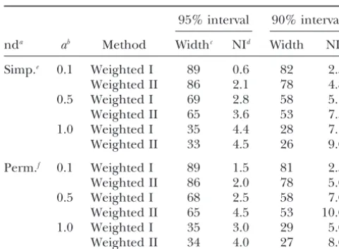
TABLE 8 though different numbers of replicates were chosen. This confirmed the finding of the low variability of the Effect of the method for calculating the null distribution
null distribution as mentioned above. on the confidence intervals for the different
In real QTL mapping experiments the permutation corrected bootstrap methods
method has become a standard to calculate the error 95% interval 90% interval probabilities. Therefore, the null distribution can be derived as a by-product without extra computational
nda ab Method Widthc NId Width NI
work. It is only necessary to retain the position of the
Simp.e 0.1 Weighted I 89 0.6 82 2.5
highest test statistic for each permutation and chromo-Weighted II 86 2.1 78 4.8 some and to ensure that this distribution covers the
0.5 Weighted I 69 2.8 58 5.1
whole chromosome. This is necessary to avoid a division
Weighted II 65 3.6 53 7.3
by zero (Equation 4). This can be done by choosing
1.0 Weighted I 35 4.4 28 7.1
either a sufficiently high number of permutations or,
Weighted II 33 4.5 26 9.0
as in the present study, by adding one estimate to those
Perm.f 0.1 Weighted I 89 1.5 81 2.5
positions not present in the initial distribution of the
Weighted II 86 2.0 78 5.0
estimates from the evaluated permuted data. In the
0.5 Weighted I 68 2.5 58 7.0
simulation, 1000 permutations were shown to be
Weighted II 65 4.5 53 10.0
1.0 Weighted I 35 3.0 29 5.0 enough to compute marker-corrected confidence
inter-Weighted II 34 4.0 27 8.0 vals for a 100-cM chromosome with six informative
markers (Table 8) when adding additional hits. The Data were simulated with a population size ofN⫽500 and
with a marker spacing of 20 cM. The chromosome length was number of permutations carried out to compute thresh-L⫽100 cM and the QTL position wasd⫽30 cM from the old values is in practice usually 10-fold higher.
start of the chromosome. Analog HPD method: The use of the analog HPD
aNull distribution.
method to compute noncentral confidence intervals led
bQTL effect, expressed in units of the polygenic standard
to a reduced width and a reduced conservativeness of deviation.
cAverage width (in centimorgans) of the confidence
in-the intervals not only when in-the QTL was located closer
terval. to one end but also when located in the middle of
dNoninclusion rate, the rate of the confidence intervals that
the chromosome (Table 5). Intuitively one would not do not contain the real QTL position.
expect significant differences between central and
eNull distribution calculated and simplified by setting the
recombination rate between the QTL and each marker to 0.5. noncentral intervals when the QTL is in the middle of The number of bootstrap samples was 250 and the number the chromosome and the markers are located symmetri-of replicates was 1000 for these genetic configurations. cally on the chromosome. The likely explanation is that
fNull distribution calculated by permuting the phenotype
the bootstrap distributions, whether corrected for the data while keeping the genotype data constant. The number
markers or not, are tailed equally only in exceptional of permutations was 1000 for each replicate. The number of
replicates for each genetic configuration was limited to 200. cases, regardless of the position of the QTL (not shown). A prerequisite for the analog HPD method to compute shorter confidence intervals is that the bootstrap distri-data and was calculated for each replicate individually.
bution is not tailed equally (seeappendixandBoxand To avoid a frequency of zero in the null distribution it
Tiao1992). was assumed that each position on the simulated
chro-Conclusions: In summary, it was shown that in the mosome would receive at least one QTL position
computation of bootstrap confidence intervals for esti-mate from the evaluation of the permuted data. The
mated QTL locations it is useful, first, to correct the population size was N ⫽ 500, marker spacing was 20
bootstrap linkage distribution for the marker impact and, cM, the QTL was put atd⫽30 cM, and the QTL effects
second, to calculate noncentral intervals. Therefore, the were a ⫽ 0.1, 0.5, and 1.0, respectively. To save CPU
use of the weighted method II is recommended, which time the total number of replicates for each genetic
combines the properties of the marker correction by configuration was limited to 200. The confidence
inter-the weighted method and inter-the properties of inter-the compu-vals were calculated with the weighted methods I and
tation of noncentral intervals by the analog HPD method. II as described above and the obtained results were
The numerical results of the simulation showed that compared with the corresponding genetic
configura-this method produced the shortest confidence intervals tion in the initial simulation, where the null distribution
while maintaining approximately the noninclusion rate was derived in a simplified manner. The results are
at 1 ⫺ P for a wide range of simulated genetic con-presented in Table 8 and show that there were no
sig-figurations. Provided permutation testing is used in an nificant differences between the two simulated series
al-experiment, this method does not require extra compu-though the null distribution was built out of 1000 estimates
tational work in comparison to the original bootstrap when computed with the permutation method, compared
1998 Mapping quantitative trait loci for milk production and
and the bootstrap approach can be termedpermutation
health of dairy cattle in a large outbred pedigree. Genetics149:
bootstrapping. 1959–1973.
This study has benefited enormously from the critical comments Communicating editor:C. Haley of two anonymous referees. It was supported by the German Cattle
Breeders Federation (ADR) and the German Ministry of Education, Science, Research and Technology (BMBF).
APPENDIX: THE ANALOG HPD METHOD
BoxandTiao(1992) define a HPD region as a region in which the probability density of every point inside is LITERATURE CITED
at least as large as that of any point outside. The analog Box, G. E. P.,andG. C. Tiao,1992 Bayesian Inference in Statistical
HPD method was adapted from the standard HPD to
Analysis.Wiley Classics Library, New York.
Churchill, G. A.,andR. W. Doerge,1994 Empirical threshold compute noncentral confidence intervals from the
dis-values for quantitative trait mapping. Genetics138:963–971. tribution of the best QTL estimate (from the linkage
Conneally, P. M., J. H. Edwards, K. K. Kidd, J. M. Lalouel, N. E.
distribution in the uncorrected method II and from Mortonet al., 1985 Reports of the committee methods of
link-age analysis and reporting. Cytogenet. Cell Genet.40:356–359. the corrected distribution in the weighted method II, Darvasi, A., A. Weinreb, V. Minke, J. I. WellerandM. Soller, respectively). When the distribution was not tailed
1993 Detecting marker-QTL linkage and estimating QTL gene
equally these intervals were noncentral because unequal
effect and map location using a saturated genetic map. Genetics
134:943–951. parts were subtracted from each tail. In contrast to the De Koning, D. J., P. M. Visscher, S. A. KnottandC. S. Haley,1998 standard HPD method it does not make any assumptions
A strategy for QTL detection in half-sib populations. Anim. Sci.
regarding the form of the distribution, whether it is
67:257–268.
Efron, B.,1979 Bootstrap methods: another look at the jackknife. unimodal or even multimodal. If the distribution has
Ann. Stat.7:1–26. the latter form the initial definition of a HPD region
Efron, B.,1982 The Jackknife, the Bootstrap and Other Resampling Plans.
cited above does not hold.
Society for Industrial and Applied Mathematics, Philadelphia.
Efron, B.,andR. B. Tibshirani,1993 An Introduction to the Bootstrap. The 95 and 90% confidence intervals were calculated
Chapman & Hall, New York. iteratively as follows:
Haley, C. S.,andS. A. Knott,1992 A simple regression method for mapping quantitative trait loci in line crosses using flanking
1. Draw a line parallel to thex-axis (the simulated
chro-markers. Heredity69:315–324.
mosome) with an initial low value ofε(the distance Hyne, V., M. J. Kearsey, D. J. PikeandJ. W. Snape,1995 QTL
analysis: unreliability and bias in estimation procedures. Mol. between the line and thex-axis), label the position Breed.1:273–282.
of the x-axis from the lower outstanding intercept Knott, S. A., J. M. ElsenandC. S. Haley,1994 Multiple marker
point between the distribution and the line astoand
mapping of quantitative trait loci in half-sib populations.
Proceed-ings of the 5th World Congress on Genetics Applied to Livestock the corresponding position from the upper outstand-Production. Vol. 21. Guelph, Canada, pp. 33–36.
ing intercept point astu.
Lander, E. S.,andD. Botstein,1989 Mapping Mendelian factors
2. Calculate the sum of the frequencies of the
distribu-underlying quantitative traits using RFLP linkage maps. Genetics
121:185–199. tion left fromtoand right fromtu,
Lebreton, C. M.,andP. M. Visscher,1998 Empirical nonparamet-ric bootstrap strategies in quantitative trait loci mapping:
condi-sum⫽
兺
to
i⫽1
f(i)⫹
兺
L
i⫽tu f(i),
tioning on the genetic model. Genetics148:525–536.
Mangin, B.,andB. Goffinet,1997 Comparison of several confi-dence intervals for QTL location. Heredity78:345–353.
Mangin, B., B. GoffinetandA. Rebai,1994 Constructing confi- wheretoandtuare the positions of thex-axis from the
dence intervals for QTL location. Genetics138:1301–1308. lower and upper intercept points between the
distribu-Martinez, O.,andR. N. Curnow,1992 Estimating the locations
tion and the parallel line, respectively, and L is the
and the sizes of the effects of quantitative trait loci using flanking
markers. Theor. Appl. Genet.85:480–488. length (in centimorgans) of the chromosome. Numerical Algorithms Group,1990 The NAG Fortran Library
Man-ual.Numerical Algorithms Group Ltd., Oxford. 3. Decide three possible cases: Reinsch, N., 1999 A multiple-species, multiple-project database
for genotypes at codominant loci. J. Anim. Breed. Genet.116: Case 1. The sum is smaller than the given error rate
425–435. of 1 ⫺
P. In this case repeat steps 1 and 2 SAS Institute,1992 SAS Language, Version 6, Ed. 1. SAS Institute,
with a marginally increased value of ε, and
Cary, NC.
Van Ooijen, J. W.,1992 Accuracy of mapping quantitative trait loci label the new positions of to and tu subse-in autogamous species. Theor. Appl. Genet.84:803–811. quently as t⬘
oandt⬘u, respectively.
Visscher, P. M., R. ThompsonandC. S. Haley,1996 Confidence
Case 2. The sum is equal to the given error rate of
intervals in QTL mapping by bootstrapping. Genetics 143:
1013–1020. 1 ⫺ P. The lower interval endpoint is the Walling, G. A., P. M. VisscherandC. S. Haley,1998 A comparison position oft
oand the upper interval endpoint
of bootstrap methods to construct confidence intervals in QTL
is the position oftu. The frequencies of both
mapping. Genet. Res.71:171–180.
Walling, G. A., P. M. Visscher, L. Andersson, M. F. Rothschild, interval endpoints are equal. See Figure A1A. L. Wanget al., 2000 Combined analyses of data from quantita- Case 3. The sum is greater than the given error rate tive trait loci mapping studies: chromosome 4 effects on porcine
of 1⫺Pand too much was subtracted from
growth and fatness. Genetics155:1369–1378.
iteration start step 1 again with a lower initial the position oft⬘oand the upper endpoint (ue)
is that point where value ofε. If it is not the first round of
itera-tion this is not caused by a too low value for
ε(a marginally lower value forεwould have
兺
t⬘oi⫽1
f(i)⫹
兺
L
i⫽ue
f(i)⫽1⫺P. resulted in case 2 and not in case 1 in the
previous round of iteration); it is caused by
This formula has to be solved iteratively. How-the form of How-the distribution, which is in this
ever, if ⌬2⬍ ⌬1, then the upper interval
end-case not unimodal. To determine the interval
point is the position of t⬘uand the lower
end-endpoints, two differences (⌬1and⌬2) must
point (indicated by le) is that point where be calculated:
兺
le i⫽1f(i)⫹
兺
L
i⫽t⬘u
f(i)⫽ 1⫺ P. (A1)
⌬1⫽t⬘o⫺ to
⌬2⫽tu⫺ t⬘u.
Again, this formula must be solved iteratively. See also Figure A1B.
If⌬1 ⬍ ⌬2 then the lower interval endpoint is
Figure A1.—Calculating confidence intervals from bootstrap distributions with the analog HPD method. (A) The hypothetical distribution is uni-modal. The lower and upper interval endpoints are built by positions on the simulated chromo-some oft⬘oandt⬘u, respectively. (B) The
hypotheti-cal distribution is not unimodal. The upper inter-val endpoint is the position oft⬘uand the position