On Geometric Control Design for Holonomic and Nonholonomic Mechanical Systems

(1)

OSBORNE, JASON, MATTHEW.On Geometric Control Design for Holonomic and Nonholonomic Mechanical Systems. (Under the direction of Dr. Dmitry Zenkov.) Geometric mechanics as a field of study does not hesitate to draw upon foun-dational geometry for formulation, re-formulation and inspiration. Herein, we take

geometry to mean not only Riemannian and differential geometry but also fibre bun-dle theory. Broadly and simply stated, an overarching and unifying theme for this document is that:

Viewing mechanical systems through a geometric lens opens up an ex-tensive set of tools that can be brought to bear upon energy, mass, and system–conscious control design for constrained mechanical systems.

To demonstrate this thesis we consider the dynamics and control for several mechan-ical systems.

(2)

revolute joint. A Riemannian structure for the double gimbal system is derived from its kinetic energy tensor which is itself constructed from the gimbal mass properties. At this point, the double gimbal system is now in the control domain of our geodesic– based PD control logic. The free and minimal energy motions of the double gimbal (or the double gimbal geodesics) are the natural tendencies of the double gimbal system that take into account its mass distribution. Since double gimbal geodesics are central to our PD control design, we work with, rather than against, the gimbals natural tendencies.

The foundational geometries most often chosen to begin modeling mechanical sys-tems are the tangent and cotangent bundles to a configuration manifold Q, denoted T Q and T⋆_Q _{respectively. That both} _T⋆_Q _and _{T Q} _{are associated bundles to the}

(3)

(4)

Biography

Jason Osborne tried to nominate his first person to write his biography, but he was politely turned down. Despite pleas as to the obvious awkwardness of relaying in-formation as a third person that only the first person can know, his first person was steadfast in the matter.

Jason Osborne was born in Fairbanks, Alaska in 1977; his father Larry was part of an Army meteorological team stationed there to gather high altitude wind data. Despite several attempts by his mother Margie to explain the series of transplantations leading them (and his sister Stacey) to Tennessee, the spacetime gel never quite set for him...

...he recalls long bus rides to school and the delightful satisfaction of shoot-ing BB’s at tin cans from his grandparents porch inx0 =Oklahoma...∆t= t1...

....he remembers wading through creeks, flipping over rocks in search of crawdads and the oppressing humidity (which, to this day and forever after, he despises) in x1 =Lousiana...∆t=t2...

....he recalls long car rides at night accompanied by NPR’s Prairie Home Companion and All Things Considered (which he hated then but would grow up to enjoy very much) and a deliciously cold snocone on the day the space shuttle landed inx2 =Whitesands, New Mexico....∆t =t3...

(5)

fly off, garbage pail kids and his first taste of freedom (walking to school through the woods [despite his mother’s admonitions]) in x3 =Fort Meade, Maryland...∆t=t4...

...he recalls Betty the bus driver (he would come to love riding the bus and would view it as a wonderful time to think and collect his thoughts) and more freedom in the form of skateboards, bicycles, basketball, tennis, wallball and football played with all the neighborhood kids until dark each day throughout their domain around Seminole drive inx4 =Johnson City, Tennessee.

Jason graduated from Science Hill High School where his interest in science (specif-ically biology) was encouraged by Mrs. Bowman. Since his bus arrived to school 30 minutes before the start of the school day, she would arrive to the classroom to find him waiting to ask questions about the previous nights readings on photosynthesis or whatever. To her credit, and a quality that he would find present in each of those professors most influential on him, she would patiently address each question in a way that would encourage more thought on his part.

(6)

Thirty years after his birth, Jason graduated from North Carolina State Uni-versity with a Ph.D. in mathematics. This third person cannot come close to re-laying the wonderful times Jason had at graduate school...the experiences were too broad...##overflow##_{...and the growth too exponential...}##overflow##_{....to be}

cap-tured by a linear net. Suffice it to say that the long days were filled with studying, teaching, basketball, movies, traveling, sculpting, painting, and studying.

(7)

Acknowledgments

Please do not read any intention into any ordering of names or statements below.

Since there are a lot of people to thank and since all of my organizational energies

went into the dissertation itself, I feel justified and liberated to write on the fly.

To say that I am extremely grateful to my many teachers and professors is a gross un-derstatement. Thank you Mrs. Bowman, Mrs. Durham, Mr. Mauldin, Mrs. Moody; Dr. Jeff Knisley, Dr. Don Luttermoser; Dr. Arkady Kheyfets, Dr. Ron Fulp, Dr. Larry Norris, Dr. Dmitry Zenkov.

I would like to single out Drs. Knisley, Fulp, and Norris for their thought and care in laying out a lucid big–mathematical–picture–to–interesting–physical–example curriculum. Each class came to represent a small piece in a large mysterious puzzle that, once started, was impossible for me to put down. Being slow at puzzles, I am truly grateful to you all for your patience and support.

I want to thank all of my committee members for giving me their valuable time. I want to thank my advisor, Dr. Dmitry Zenkov, for his course on mechanics that added extra dimensionality to the mystery puzzle. Exploring these corners has provided many interesting problems and opportunities. For his support at each stage of the whole dissertation process and for the career development opportunities he (through the NSF) supported, I cannot be more thankful. For the headaches I know I caused him as he kindly dragged me into the world of multi–tasking, I am sorry.

(8)

cellphone for making the hours long conference calls and “that” never–ending article possible.

For all sorts of random help too numerous to relay, my deepest thanks go to Brenda Currin, Di Bucklad, Denise Seabrooks, Carolyn Gunton, Charlene Wallace, Seyma Bennett–Shabbir, Frankie Stephenson and Janice Gaddy.

To Ali, Brandon and Chirag thanks for the Cup–A–Joe–India–Garden nights where ideas were let fly.

To the houseoffive (Brian Adams in particular), for the college dorm and roommate experience I never had.

To every coffee shop with free wireless in which I have spent countless hours, thank you.

To Mitch’s limeade, turkey sandwiches, black bean chili, and Lisa, thank you so much for providing a cool (temperature) and unique environment in which to study for qualifying exams.

My deepest gratitude goes to Catherine Daubert for making me aware of the NC State Craft Center; had you not suggested that first class I really have no concept of where I would be today. Thanks to the NC State Craft Center for providing the excellent studio space for me to work in while I recovered my sense of balance after my qualifiers. I would like to express my gratitude to Jock Gault for the excellent figure sculpture classes wherein he let me find my own path (with gentle nudges every once in awhile). To Jim Fatata, I thank you for the use of your studio space and the many helpful pointers.

To Amme Klose, your unedited truthfulness, spontaneity and constant friendship brings to mind

a vinyl blue

folding chair in the sun

(9)

To Susan Mahar, wherever in the world you are now, thank you for more than I can say. In my mind you conjure the only poem (if i by ee cummings) that ever really struck me to the point of remembering

...i say to hell with that i

say that doesn’t matter) but if somebody

or you are beautiful or deep or generous what i say is

whistle that

sing that yell that spell

that out big (bigger than cosmic rays war earthquakes famine...

To Karey Markovich, wherever in the world you are now, attempting to cook noodles on the dash of your car using the sun, experiencing the profound silence of Haleakala and driving along the bumpy north side of Maui are experiences I will never forget. Thank you for your hospitality, friendship and generosity.

To Paddy, Frank, Dr. Griggs and the various incarnations of (the original) LaceEmUp, I would not trade the memories of lunchtime basketball, one–on–one-on–one games of 21 and our two championships for anything, not even for a theorem with my name on it. Thank you all.

To Jill Reese, for the (mis)adventures we have already had and the many more we have yet to experience, I want to say that “You are my biker”.

(10)

List of Tables

3.1 Geometric data for the double gimbal torus. The mass matrix entries mij are substituted into eq. (A.32) to find the Christoffel symbols, Γijk

which are substituted into eq. (A.16) to lead to the functionRijkl. The

Gauss curvature,K is then computed by the above equation. . . 71 3.2 Geodesic information for the double gimbal. For a double gimbal

with inertia data given in the left column, the geodesic types ( par-allel, meridian, bound or asymptotic) are indicated. . . 72

(15)

List of Figures

1.1 Chaplygin Sleigh and Double Gimbal System . . . 5

2.1 The Chaplygin sleigh (top view of Figure 1.1(a)) . . . 18

2.2 The momentum dynamics of the unbalanced sleigh. . . 20

2.3 A generic trajectory of the contact point. . . 21

2.4 Control Primitives for Chaplygin Sleigh. (a) Transition form a circle to the trajectory with desired direction (b) Transition from a generic trajectory to a circle (c) Transition from a straight line to a generic trajectory. . . 26

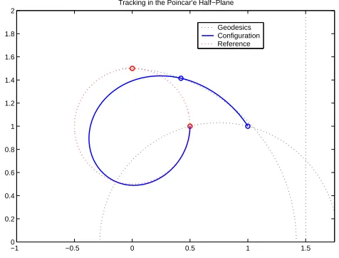
3.1 Tracking a circular trajectory in the Poincar`e Plane . . . 58

(16)

3.3 Some geodesics on the double gimbal torus. The black curves are the gimbal geodesics γ(u) = (θ(u), φ(u)) mapped under T given in (3.12) and plotted on the surface defined by the image of T. The parallel, asymptotic and bound geodesics seen here are typical of any inertias fitting the description of the second line of Table 3.7. In this particular case, the inertias are in the ratio Iz = 2, Jz = 2, Jx = 1, Jy = 4

with initial conditions [θ = 0, φ = π/2,θ˙ = .8164965808,φ˙ = 0],[θ = 0, φ = 0,θ˙ = .6123724355,φ˙ = .3535533910] and [θ = 0, φ = 1,θ˙ = .7794529900,φ˙ = 0] for the parallel, asymptotic and bound geodesics, respectively. A geodesic on the double gimbal torus is a minimal energy

motion (time evolution absent external forces) of the double gimbal system. . . 69 3.4 Asymptotic Motion. The motion of the double gimbal system

(17)

3.5 The flat double gimbal. An example of the ”flat” double gimbal sys-tem is constructed by mounting a uniform, spherically symmetric body (denoted J) to the outer gimbal. Since the ratio Jz/Jx equals 1, the

mass matrix of (3.14) becomes angle independent and thus the “flat” gimbal inherits its flatness from an angle independent kinetic energy metric. The angle independent metric of the flat gimbal has the ef-fect of decoupling the inner and outer gimbal free motions (see Figure 3.7). Since it is geometrically straight forward to analyze, the flat double gimbal gives an intuitive and simple example into not only the behavior but also the control of more difficult (meaning ”non-flat” or coupled) double gimbal systems. . . 70 3.6 Klingenberg result andLokicomputations on the double gimbal torus.

The blue geodesics emanate from a pointpfor a distancei(T2_{) given by} the Klingenberg result which defines the red curve. The green geodesics emanate from point p until they reach the two black rings called the cut locus C(p) as determined by the softwareLoki. For inertia–based tracking control of the double gimbal system, the region described by the red curve is a conservative estimate of the region of local exponen-tial stability. For fixed–point to fixed–point maneuverers, the black rings, are the problematic reference configurations for local exponen-tial stability of our inertia–based PD control logic. . . 70 3.7 Fixed–point to fixed–point tracking on double gimbal torus. The geodesic

segments given in black are the minimal energy motions between two successive double gimbal configurations. That the cut locus is avoided for each point along the geodesics indicates that our inertia–based PD control design is valid and proceeding in an energy efficient manner. . 71

(18)

A.2 Parallel Transport on Euclidean R3 _{and standard S}2_{. a) (left) For} R3 the curve is γ(u) = [x(u), y(u), z(u)] = [sin(u),cos(u), u] is given in black with initial vector V0 = [0,0,1] (time u0 = 1) given in blue and the transported vector Vf = [0,0,1] (time uf = 7) given in green. b)

(middle) For S2 _{the curve} _{σ(u) =}_{S(u, u) is given in black with initial} vector V0 = [1,1] (time u0 = 1) mapped to the curve σ(u) under DS given in blue and the transported vector given in green (timeuf = 3).

c) (right) Parallel transport of initial vector,V0 (in blue) around closed curve (in black) to a final vector,Vf (in green) . . . 135

B.1 Adapted Coordinates on Q from a Local Trivialization of a Local Section137

I.1 Control of moving frame along the geodesic using the control input vectorA = [₋1,₋1,1]. . . 217 I.2 Typical trajectory of particle whose z–velocity is nonholonomically

con-strained by ˙z=yx˙ . . . 219 I.3 The particles motion towards negative infinity can be arrested and we

can return the particle to its starting position. The necessary input data is Cx = −0.1, Cy = −0.1, Cz = 0, xref = yref = zref = 0, IC:

[x0, y0, z0,x0,˙ y0] = [0,˙ 0,0,1,₋1]. . . 220 I.4 The particles motion towards negative infinity can be arrested and we

can redirect the particle in a “perpendicular” and “elevated” direction. The necessary input data is Cx = 0, Cy = −1, Cz = 0, xref = yref =

zref = 0 (left),xref =yref =zref = 0.1t(right), IC: [x0, y0, z0,x˙0,y˙0] = [0,0,0,1,₋1]. . . 220 I.5 Using a cyclic reference point, the particle can be given momentum

and thus move away from equilibrium. The necessary data input data is Cx = −0.1, Cy = −0.1, Cz = 0, yref = zref = 0, xref = sin(t), IC:

(19)

Notation

M(orQ) n-Dimensional (configuration) manifold . . . 31

(qJ ) J= 1..dim(Q) =n Coordinates on Q . . . 31

TqQ Tangent space to Q atq. . . 31

ˆ ΩI n-Symplectic vector valued–two form defined by dθˆI_{. . . 74}

∆_θ_ˆI _{Distribution adapted soldering form . . . 76}

∆⋆ _{(n-m)-dimensional co-distribution on Q . . . 86}

∆ m-dimensional distribution on Q defining system constraints . . . 87

X(M) Set of smooth vector fields on M. . . .105

F(M) Set of smooth real-valued functions on M . . . 105

X, Y Typical elements of TQ or X(Q) . . . 105

S =Q/G Symmetry reduced (shape) manifold . . . 137

(ri₎ _i_{= 1..dim(Q/}_G_{) Coordinates on} _Q/_G_{. . . 137}

G Lie group . . . 138

(sA₎ _A _{= 1}_{. . .}_dim(_G_{) coordinates on}_G_{. . . 138}

LQ Frame bundle of Q . . . 139

u= (q, f) Reference frame on LQ . . . 140

u= (q, e) Arbitrary element of LQ. . . .140

ΠI J Canonical coordinates on LQ . . . 141

u= (q, ∂) Canonical reference frame on LQ . . . 141

∆ Π I J Distribution Adapted Coordinates on LQ . . . 141

T Q Tangent bundle of Q; vector bundle associated to LQ. . . 143

(20)

E(P, V) Vector Bundle associated to P with fiber V . . . 145

[u, v] Equivalence class element of T Q viewed as LQ_⊗Gl(n)Rn . . . 146

T⋆_Q _{Cotangent bundle of Q; Vector bundle associated to} _LQ_{. . . 147}

[u, α] Equivalence class element of T⋆_Q _{viewed as} _LQ_⊗ Gl(n)Rn⋆. . . 147

Tr_s(M) Set of r-contravariant and s-covariant smooth tensor fields on M . . 149

ˆ θI Soldering vector–valued one–form on LQ . . . 156

ϑ Canonical real–valued one–form on T⋆_Q_{. . . 156}

LπQ Vertically adapted frame bundle of Q→π Q/G. . . 168

L∆Q Distribution adapted frame bundle of Q . . . 171

u= (q,F∆) Distribution adapted reference frame on LQ . . . 172

g Lie algebra of G. . . 192

ξ, η Typical Lie algebra elements . . . 193

(21)

Introduction

1.1 Selective Historical Excerpts

A relatively brief venture into the history of late nineteenth and early twentieth century mathematics, specifically the development of Lie groups [17], brought clearly and to the forefront of my attention that many great mathematicians were inspired by the advances in the physics of their time. Indeed, Hermann Weyl wrote (1949, [17, pg. 421])

For myself I can say that the wish to understand what really is the math-ematical substance behind the formal apparatus of relativity theory led me to the study of representations and invariants of groups...

where (general) relativity theory is the theory of gravitation developed by Albert Einstein in 1916. According to ([17, pg. 423]) and the references cited therein, Ein-stein began the 1916 paper by acknowledging a debt to the mathematician Hermann Minkowski:

The generalization of the relativity theory was facilitated through the form that Minkowski had given to the special relativity theory. He was the first mathematician to clearly perceive the formal equivalence of the

(22)

space and time coordinates; this made possible the construction of the [general] theory.

The form of special relativity theory, as mentioned above by Einstein, with roots in James Clerk Maxwell’s electromagnetic theory of light, is based upon the equal treatment of both space and time. In Minkowski’s own words (1907, [17, pg. 339])

Out of the electromagnetic theory of light there recently seems to have come a complete transformation of our representations of space and time which must be of exceptional interest to the mathematician. The mathe-matician is also especially well prepared to pick up the new views because it is a question of acclimatization to conceptual schemes with which he has long been familiar. The physicist meanwhile must rediscover these concepts and must painfully cut way through a primeval forest of obscu-rities.

Embedded in the above quote is the call for mathematicians to look to physics for interesting problems that they are, by their training, well equipped to solve. The necessity of such a statement and why Minkowski would jestingly need to apologize in a letter to David Hilbert for being

. . . thoroughly infected with physics . . .

gains meaning through an understanding of the mathematical atmosphere of the late 19th _{century. As stated by the author in ([17, pg. 334]):}

(23)

That Newtonian (foundational) mechanics was the science of the time for Euler and Lagrange no doubt influenced Hilbert’s feelings that it would be

very desirable that the discussion of the foundations of mechanics be taken up by mathematicians also. (1900, [17, pg. 334])

Given the advice of this great mathematician, one can feel the sense of bewilderment in the anonymous quote from the preface of [24] published in 1992!

Many of the greatest mathematicians—Euler, Gauss, Lagrange, Riemann, Poincare’, Hilbert, Birkoff, Atiyah, Arnold, Smale— were will versed in mechanics and many of the greatest advances in mathematics use ideas from mechanics in a fundamental way. Why is it no longer taught as a basic subject to mathematicians?

On a personal note, it has been my experience that the clear take home message from those historically minded individuals to those not-so historically interested is ubiquitously “learn your history so you are not doomed to repeat it”. Regarding the mathematical study of mechanics, I have at least begun to learn my history for the following document reflects my efforts in the study ofgeometric mechanics.

In the next section we summarize more recent literature which play a central role to our contributions in geometric mechanics, specifically control design of holonomic and nonholonomic mechanical systems.

1.2 Literature Background and Statement of

Con-tributions

This document largely addresses geometric control design for holonomic and non-holonomic mechanical systems and is centrally based upon the following foundational framework:

(24)

B: PD (proportional and derivative) feedback control on manifolds as introduced in Bullo et. al. [9] and further developed in Bullo [6],

C: n-Symplectic geometry (generalized cotangent bundle geometry) and n-symplectic dynamics (generalized Hamiltonian dynamics) as developed in [28].

A zeroth order statement of this documents contributions are as follows:

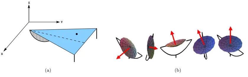
A’: We show that the Chaplygin sleigh, a rigid platform with attached blade (im-posing nonholonomic constraints, see Figure 1.1) can be steered using a moving mass, see Chapter 2 and Osborne and Zenkov [31]. The dynamics of the sleigh are a special case of those derived in [3].

B’: Using geometric constructs (geodesic distance and parallel transport), we spe-cialize the PD control theorem of [6] to a class of Riemannian manifolds, see Chapter 3 and Fuentes, Hicks and Osborne [14] and [15]. We specifically apply our controller to the double gimbal system, a coupled system of rigid bodies (see Figure 1.1).

C’: As an alternative to the tangent bundle (Lagrangian) and cotangent bundle (Hamiltonian or symplectic) formulations of mechanics, we demonstrate the frame bundle (n-symplectic/moving frame) approach to nonholonomic mechan-ical systems with symmetry. An n-symplectic equivalent of the nonholonomic momentum equation of [3] is obtained and the feasibility of momenta based control design is established.

(25)

Z

000000000000000000000 000000000000000000000 000000000000000000000 000000000000000000000 000000000000000000000 000000000000000000000

111111111111111111111 111111111111111111111 111111111111111111111 111111111111111111111 111111111111111111111 111111111111111111111

X

Y

(a) (b)

Figure 1.1: Chaplygin Sleigh and Double Gimbal System

1.2.1 Short Summary of BKMM [3]

The dynamics of nonholonomic mechanical systems with symmetry are obtained in [3] using a constrained form of the Lagrange–d’Alembert principle, i.e. where both velocities and the variations are constrained. Utilizing also Lagrangian reduction techniques the constrained, reduced dynamics become the so called (nonholonomic) momentum equation which can be expressed as

˙

p=_hα(r)p, p_i+_hβ(r)p,r˙_i+_hγ(r) ˙r,r˙_i (1.1)

and theshape equation which can be expressed as

¨

r =f(r,r, p).˙ (1.2)

The shape equation is of Euler-Lagrange type on the reduced space with extra forc-ing terms. Together with the reconstruction equation or group dynamics equation expressed as

˙

g =g(J(r)p₋A(r) ˙r), (1.3)

these three equations are the full system of equations for nonholonomic mechanical systems with symmetry. See [3] for a derivation and the coordinate form of these dynamics or [16] for a coordinate free (bundle and connection oriented) approach.

(26)

and momentum dynamics are coupled, they are both decoupled from the group dy-namics. The momentum equation characterizes a major difference between holonomic and nonholonomic systems. According to Noether’s theorem, for a holonomic system with symmetry, the spatial components of momentum are conserved. On the con-trary, for nonholonomic systems the momenta are, in general, dynamic variables with dynamics governed by a nontrivial momentum equation. The nonholonomic momen-tum equation and its lack of conservation are shown to be important in control, motion generation, and stability analysis of nonholonomic systems (see Bloch et al. [3], Zenkov et al. [41], and references therein).

That the nonholonomic momenta are not, in general, conserved and that the nonholonomic momenta dynamics are coupled to the shape dynamics allows us to restate our first contribution more precisely:

Contribution A’ restated: We design a steering control algorithm for the Chaplygin sleigh using a moving mass. The key to the design lies in certain control primitives that are discovered from an analysis of the momentum equation (2.2) for particular fixed placements of the mass. Assuming fully actuated control over the moving mass (the shape of the system) and utilizing the coupling between shape dynamics and nonholonomic momentum equation we are able to asymptotically steer the sleigh to any desired direction of motion and to any point in the plane.

(27)

1.2.2 Short Summary of Bullo et.

al.

[9] and Bullo and

Murray [6]

By way of two simple and yet illustrative examples we can gain a partial footing into the PD control results of Bullo and thusly to our specialized geometric PD control result.

Simply stated, to render the dynamics of a system in PD (proportional plus deriva-tive) form is to add control forces to the systems free dynamics for which the controlled dynamics take the form of a damped, linear spring. For a point particle of mass m moving in 1D, the free/uncontrolled dynamics aremq¨= 0. Introduction of the control forces 1) the negative gradient of a positive definite quadratic potential 1₂kq2 _about q= 0; the proportional control forces and 2)the damping constant times the velocity cq; the˙ derivative control forces renders the free point particle dynamics of the form mq¨+cq˙+kq= 0. Adjusting or tuning the control parameters k, c, one can make the particles position asymptotically approach q= 0 with zero velocity ˙q= 0.

Extending the 1D damped spring example to mechanical systems with configura-tion manifold Q is the over arching idea behind [9] and [6]. A mechanical system of particular interest to us is the double gimbal system (see Figure 1.1). Simply stated, the double gimbal system is comprised of a base, an outer gimbal attached to the base through a revolute joint, and an inner gimbal attached to the outer gimbal also through a revolute joint. Since this system has two circular degrees of freedom, the spinning angles of both the inner and outer gimbals, the configuration manifold is the torus T2 ₌ _S1_×_S1_{. Equipping the torus with the kinetic energy metric defined by} the mass properties of the inner and outer gimbals, we obtain a Riemannian manifold that we call the double gimbal torus. Control on the double gimbal torus takes two flavors(a)fixed point trackingwhich corresponds to re-orientating a telescope pointed at fixed Star X to fixed Star Y and (b)full tracking which corresponds to a telescope tracking a comet.

(28)

energy curve (a geodesic) connecting the points identified with Star X and Star Y and (2)a dissipation force opposing motion along a geodesic segment which will eventually stop the telescope when pointed at Star Y.

In Bullo et al. [9] the geodesic based PD fixed point tracking controller intuitively described above was introduced and implemented on the two-sphere. In the conclu-sions of Bullo et. al., it is stated that design of Lyapunov functions for tracking on not only the sphere and Lie groups but also a general Riemannian manifold are problems of future interest. Indeed, in Bullo and Murray [6] a general PD feedback control law was formulated for tracking on Riemmanian manifolds. The general feedback forces devised are analogous to those of the damped simple harmonic 1D oscillator example. It should be emphasized at this point that to actually implement the general controller of Bullo and Murray on specific examples requires the explicit formulation of the feedback forces, which themselves are constructed from explicit formulations of a compatible pair of objects called i) the configuration error andii) the transport map. Utilizing canonical cross product Lie algebra structure of R3 ∼_{= so(3), the} configuration and velocity errors are explicitly formulated in [6] for tracking on the two-sphere embedded in R3_.

Contribution B’ restated:

(29)

the software Loki _{[39], we are able to obtain estimates for the stability}

region on the double gimbal torus. With this knowledge we are able to confidently implement the controller.

The details of this contribution along with further supporting references are given in Chapter 3. This chapter was joint work with Dr. Robert Fuentes (then at, Boeing-SVS) and Dr. Gregory Hicks (then at, General Dynamics) and originally appeared in [14] and [15]. This authors work on the project was supported by the Air Force Research Labs (AFRL) Space Scholars program. During this time the author was also supported by NSF grant DMS-0306017 (PI: Dr. D. Zenkov).

1.2.3 Short Summary of LKN [28]

The geometries most often chosen to begin modeling mechanical systems are the tangent and cotangent bundles to a configuration manifold Q, denoted T Qand T⋆_Q

respectively. For example, to obtain dynamics on T⋆_Q _{one needs only a geometric}

object, a real-valued one form, ϑ called the canonical form and a physical object, a real-valued function, f called an observable or Hamiltonian function. Specifically, given the canonical real-valued one-form, ϑ on T⋆_M _{and corresponding canonical}

non-degenerate real-valued two form Ω =dϑ onT⋆_M _{given in canonical coordinates}

(qi_{, p}j_{) by}

Ω =dpi∧dqi (ϑ=pidqi) (1.4)

one can use the structure equation

df =₋Xf Ω (1.5)

to uniquely determine a global Hamiltonian vector field Xf given a globally defined

Hamiltonian function f : T⋆_M _→ _R_{. The integral curve equations of the global}

Hamiltonian vector field are exactly Hamilton’s equations.

(30)

bun-dle of linear frames) of a configuration manifold Q, denoted LQ seems to, at least initially, indicate that LQ is also a natural geometric model of mechanical systems (see Appendix B for LQdetails and Appendix C for associated bundle details). The appropriateness of LQ to the study of mechanical systems is strengthened by the discovery of the generalized symplectic (Hamiltonian) structure on LQin [28]. Using the n-symplectic structure of LQ, this reference establishes the generalized momenta dynamics for arbitrary rank observables.

For example, following [28], one obtains dynamics of mechanical systems on the frame bundle by first lifting a rank-2 observable, the kinetic energy metric g, a (0,2) tensor field on Q, to anRn_⊗Rn_{-valued tensorial function ˆ}_g _on_LQ _{and then solving} then-symplectic structure equation, a generalization of the structure equation onT⋆_Q,

dˆgij =₋2 ˆX_ˆ_g(i Ωˆj) (1.6)

for n-vector fields [ ˆXi

ˆ

g]. Here ˆΩ = dθˆwhere ˆθ is an Rn-valued generalization of the

canonical form θ on T⋆_Q _{called the} _{soldering form}_{. A critical difference in the}

n-symplectic versus the n-symplectic setting is that solutions [Xi

ˆ

g] are equivalence classes

of vector fields rather than a unique vector field. Equivalence here is characterized by ann-symplectic gauge freedom in the choice of a torsion free connection which, when specified, defines a unique solution vector field.

It is of general interest to the author to establish the applicability of n-symplectic geometry to mechanical systems and control. To the author’s knowledge, no one has considered this approach. It is both interesting and encouraging to note that linear connections, the frame bundle and the distribution adapted frame bundle (used below) make an appearance in [21], a paper whose application of affine connections and distributions is to derive the nonholonomic momentum equation. To our reading and understanding, n-symplectic geometry played no role in the derivation.

(31)

of mechanical systems perspective in mind has not been addressed.

Contribution C’ restated: For a distribution ∆ modeling a mechanical sys-tems nonholonomic constraints, weadaptthe soldering form ˆθ, the kinetic energy observable and the frame bundle to the distribution to obtain a distribution adapted structure equation

d∆g

ij

=₋2X∆ (i

ˆ

g

∆ Ω

j)

(1.7)

specific solutions to which lead to constrained momenta dynamics. Some of the momenta dynamics are the nonholonomic momentum equation of [3]. That the n-symplectic theory allows for the introduction of potentials which appear at the generalized momenta level indicate the feasibility of potential shaping and momenta based control design for nonholonomic mechanical systems. We illustrate the above n-symplectic approach using two examples, the vertical rolling hoop and a nonholonomic constrained particle.

(32)

1.3 On the Structure of this Document

There are many appendices for this document that offer extra details and relevant background material for the readers’ convenience. For Chapter 3, which utilizes a significant amount of geometry in developing a PD control logic on Riemmanian manifolds, we have added

• Appendix A which collects a detailed account of the requisite Riemmanian geometry objects and

• Appendix D which gives a detailed account of a fibre bundle needed to correctly formulate a configuration error functionfrom our PD control design.

For Chapter 4, which utilizes n-symplectic (frame bundle,LQ) geometry to formulate the dynamics for constrained mechanical systems, we have added several appendices.

• Appendix B defines the frame bundle and its fibre bundle structure.

(33)

• Appendix G, addresses the canonical formulation of generalized Hamiltonian mechanics on the frame bundle. Appendix F defines the (constraint) distribu-tion adapted frame bundle,L∆Q. The canonical dynamics and L∆Qare key to formulating the constrained n-symplectic dynamics.

• We have also added Appendix H which summarizes the nonholonomic momen-tum equation of BKMM [3] which will be compared to the generalized momenta dynamics on L∆Q.

(34)

Chapter 2 The Moving Mass Chaplygin Sleigh

In this chapter we design a steering control algorithm for the Chaplygin sleigh with a moving mass. Our strategy is to only use the controlled dynamics to initiate short-time transitions between the various uncontrolled modes of the system in order to achieve the desired direction of motion.

2.1 Introduction

The objective of this chapter is to use a moving mass to control the direction of motion of the Chaplygin sleigh—a rigid body on a horizontal plane constrained by a blade. The blade limits the velocity of the body-plane contact point to a direction fixed in the body. This constraint isnonholonomic as it imposes a velocity restriction on the system which is not derivable from a position constraint. Rand and Ramani [33] and Ruina [36] point out that blade constraints similar to this have been used to model an underwater missile with fins.

In recent years much work has been done in using geometric structures to both formulate the equations and to address aspects of control of constrained mechanical systems. We summarize some such works. For a more complete list of references on the dynamics and control of nonholonomic systems see [4].

In the seminal paper by Bloch, Krishnaprasad, Marsden, and Murray [3] (hereafter

(35)

referred to as BKMM), nonholonomic mechanical systems with symmetry are studied. For a system with symmetry, it is natural to split the configuration variables into the

group variables g which describe the overall position (attitude) of the system and the

shape variablesr which describe the positions of the system’s components relative to each other. In the case of the Chaplygin sleigh with a moving mass, the variable g is the element of the group of Euclidean transformations of the 2-dimensional plane and the variable r is the position of the moving mass relative to the contact point of the body and the plane.

The dynamics of a nonholonomic system with symmetry are governed by the system of equations

¨

r =f(r,r, p) +˙ u, (2.1) ˙

p=_hα(r)p, p_i+_hβ(r)p,r˙_i+_hγ(r) ˙r,r˙_i, (2.2) ˙

g =g(J(r)p₋A(r) ˙r), (2.3)

wherepis thenonholonomic momentum, which in general is no longer conserved, and urepresents control forces. We emphasize that the controls appear only in the shape equation. Note that equations (2.1) and (2.2) decouple from the the group dynamics (2.3). See [3] for details and formulae that define the various coefficients in equations (2.1)–(2.3). Equations (2.1), (2.2), and (2.3) are referred to as the shape equation,

momentum equation, and reconstruction equation, respectively.

Utilizing the perturbation methods of [19] to study equations (2.1)–(2.3), Os-trowski [32] determines relations between the cyclic control inputs u(t), resultant

momentum generation, and ultimately, motion. These integral relations were critical in designing momentum generating and steering algorithms.

In Lewis and Murray [23], a symmetric product is introduced and used to for-mulate sufficient conditions for various types of configuration controllability ofsimple

(36)

Simple mechanical control systems with constraintsare treated in Lewis [22]. The symmetric product was shown to address configuration controllability questions in this constraint setting also.

In Bullo, Leonard, and Lewis [7], simple mechanical control systems on a Lie group G are investigated. Here the dynamics of interest are of the form

˙

p=_hα p, p_i+uaFa, (2.4)

˙

g =g(Jp), (2.5)

where ua _{are the control inputs and} _F

a are the directions in which they act.

Imple-menting the perturbation approach of [19] and using the symmetric product technique, Bullo, Leonard, and Lewis [7] design steering control algorithms for equations (2.5) and (2.4).

The physical system of particular interest to us is the Chaplygin sleigh with a fully actuated moving mass. The dynamics of this system are of the form (2.1)–(2.3) (details are given in Section 2.2).

Unlike Ostrowski, in this paper we are not concerned with motion generation. We assume that the Chaplygin sleigh is already in motion and concentrate onsteeringthe system using the movable mass. Since the mass is fully actuated, we can assign its position relative to the sleigh as a function of time. Therefore, the dynamics reduce to equations (2.2) and (2.3), where the moving mass positionrrelative to the contact point is interpreted as the control parameter. We emphasize that the dependence of the right-hand sides of (2.2) and (2.3) on r is inherently nonlinear, and thus the control design of Bullo, Leonard, and Lewis [7] is not applicable.

The perturbation control techniques and associated algorithm design of Ostrowski [32] and Bullo, Leonard, and Lewis [7] mentioned above are extremely useful and have a wide range of application. However, it is our philosophy that the dynamics of the

(37)

Our control philosophy can be outlined as follows: We first study the variety of trajectories of equations (2.2) and (2.3) in the uncontrolledsetting (i.e.,constant r). We then use thecontrolleddynamics (i.e.,equations (2.2) and (2.3) with non-constant r) to switch between the various types of uncontrolled dynamics which then lead to the goal configuration. This approach proved to be useful in various situations (see, e.g., [5]). We emphasize that the transfer is very short in duration and hence the system remains uncontrolled for most of the steering procedure.

On a technical note, we assume that, except for the short time that the actuators must implement the change in shape configuration, they are at rest. That is, the actuators are engineered to maintain the constancy of rwhen inactive. For example, in the Chaplygin sleigh, we can view the mass as sliding on a rod where the friction between the rod and sliding mass, not the actuator, is applied to keep the mass fixed. The exposition is organized as follows: In Section 2.2 we summarize the properties of the uncontrolled dynamics of the Chaplygin sleigh. In particular, we list all possible types of trajectories of the contact point of the sleigh on the plane. In Section 2.3 we study “control primitives” which implement the transitions between the uncontrolled trajectories of the sleigh. These control primitives, when applied in the proper order, result in the desired reorientation of the system. Simulations are presented in Section 2.4.

2.2 The Dynamics of the Chaplygin Sleigh

2.2.1 The Configuration Variables

The Chaplygin sleigh is a rigid body sliding on a horizontal plane. The body is supported at three points, two of which slide freely without friction while the third is a knife edge, a constraint that allows no motion orthogonal to this edge. This mechanical system was introduced and studied in 1911 by Chaplygin [11] (although the work was actually finished in 1906).

(38)

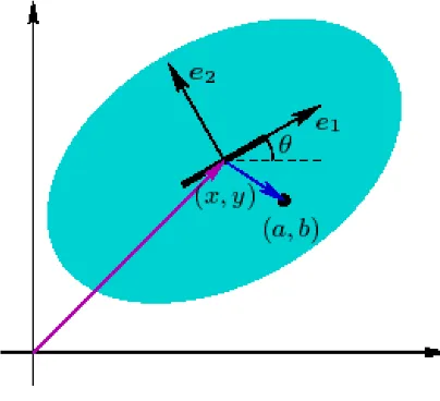
two-dimensional plane which we parameterize with coordinates (θ, x, y). As Figure 2.1 indicates,θ and (x, y) are the angular orientation of the blade (shown as the bold segment in the Figure) and position of the contact point of the blade on the plane, respectively. We view the sleigh as a platform whose center of mass is at the contact point. The mass and moment of inertia of the platform relative to the contact point areM andI, respectively. There is also a point massmpositioned at (a, b) relative to the platform, see Figure 2.1. In the classical Chaplygin sleigh this mass is motionless relative to the platform; in Section 2.3 we will control its position in order to steer the sleigh on the plane.

Figure 2.1: The Chaplygin sleigh (top view of Figure 1.1(a))

The constraint imposed by the blade reads

−x˙sinθ+ ˙ysinθ = 0. (2.6)

(39)

2.2.2 The Momentum Dynamics and Reconstruction

Let Ω1 _{be the angular velocity of the platform and Ω}2_{, Ω}3 _{be the components of} linear velocity of the contact point along and orthogonal to the blade, respectively. Constraint (2.6) implies Ω3 _{= 0.}

Denote the nonholonomic momentum by (p1, p2). The components p1 and p2 satisfy the equations

Ω1 = (M +m)p1+mbp2 (M +m)(I+ma2_{) +}_{M mb}2, Ω2 = mbp1 + (I+ma

2₊_mb2₎_p2 (M +m)(I+ma2_{) +}_{M mb}2,

see [3] and [42] for details and definitions. If b = 0, the components p1 and p2 equal the angular momentum of the sleigh relative to the contact point, and the projection of the linear momentum along the direction of the blade, respectively.

The dynamics of the Chaplygin sleigh is governed by the momentum equations

˙

p1 =₋maΩ1Ω2, p2˙ =ma(Ω1)2, (2.7)

coupled with the reconstruction equations

˙

θ = Ω1, x˙ = Ω2cosθ, y˙ = Ω2sinθ, (2.8)

(see, e.g., [42]). This representation of the equations of motion allows one to first solve (2.7) and then find the trajectory of the sleigh by integrating equations (2.8). For the details on the derivation of these equations see BKMM [3] and Zenkov and Bloch [42].

The dynamics of the Chaplygin sleigh depends drastically on the value of a. This dependence is critical in the design of our control algorithm in Section 2.3.

(40)

In both cases the contact point is moving at a constant rate. The existence of circular trajectories is very important for our steering control algorithm.

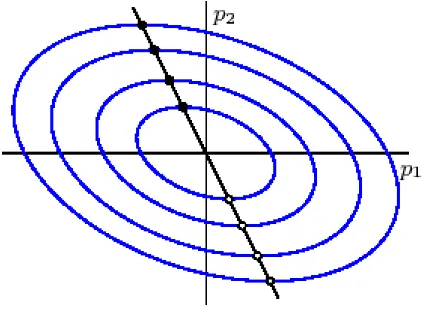
If a₆= 0, the trajectories in the momentum plane are either equilibria situated on the line (M +m)p1 +mbp2 = 0, or elliptic arcs, as shown in Figure 2.2. Assuming a >0, the equilibria located in the upper half plane are asymptotically stable (filled dots in Figure 2.2) whereas the equilibria in the lower half plane are unstable (empty dots). The elliptic arcs form heteroclinic connections between the pairs of equilibria. The trajectories of the contact point that correspond to the momentum equilibria are

Figure 2.2: The momentum dynamics of the unbalanced sleigh.

straight lines in the xy-plane. They are stable if the mass m precedes the contact point and unstable otherwise.

(41)

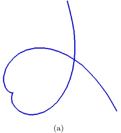
(a)

Figure 2.3: A generic trajectory of the contact point.

2.3 Controllability of the Chaplygin Sleigh with a

Moving Mass

2.3.1 The Reduced Controlled Dynamics

We now allow the point mass to change its position relative to the rigid body. That is, the quantities (a, b) are now dynamic variables. Assuming that the mass degrees of freedom are fully actuated, the system’s dynamics are given by equations (2.2) and (2.3), where r = (a, b) is viewed as the control parameter. Recall that the controller is active only when ˙a2_{+ ˙}_b2 ₆_{= 0—see the discussion of the physical implementation of} controllers in the Introduction.

In order to write equations (2.2) and (2.3) for the Chaplygin sleigh with a moving mass explicitly, let

ξ1= (M +m)(p1−mab) +˙ mb(p2+Ma)˙ (M +m)(I+ma2_{) +}_{M mb}2 , ξ2= m[b(p1−mab)˙ −(I+ma

2_{) ˙}_{a] + [I}₊_m(a2₊_b2_)]p 2 (M+m)(I+ma2_{) +}_{M mb}2 , and define η by

(42)

The momentum dynamics (2.2) for the Chaplygin sleigh with a moving mass is com-puted to be

˙

p1 =₋mηξ2, p2˙ =mηξ1. (2.9) Observe that for (a, b) = const, equations (2.9) reduce to (2.7).

After solving equations (2.9), the group configuration variables (θ, x, y) are ob-tained from the reconstruction equations

˙

θ=ξ1, x˙ =ξ2cosθ, y˙ =ξ2sinθ.

2.3.2 Controllability of Asymptotic Directions

Recall that if (p1, p2) is constant andp2 6= 0, there are three types of motions for the uncontrolled ( ˙a2_{+ ˙}_b2 _{= 0) dynamics:}

1. If a ₆= 0 and (M +m)p1 +mbp2 ₆= 0, then the system’s trajectory is a curve that approaches straight-line motions ast _{→ ±∞}(see Figure 2.3).

2. If a = 0 and (M +m)p1 +mbp2 ₆= 0, then the system moves along a circle in the xy-plane at a constant rate.

3. If (M+m)p1+mbp2 = 0, the system moves along a straight line in thexy-plane at a constant speed.

(43)

Theorem 2.3.1 Assume that the initial motion of the system is circular, i.e., a= 0, b= const, and (M+m)p1+mbp2 ₆= 0. Then there exist a continuously-differentiable function a(t) and constants A, T1, and T2 with properties

• a(t) = 0 when t _≤T1 and a(t) = A when t_≥T2,

• a(t) is increasing when T1 < t < T2,

such that the trajectory of the system with a = a(t), b = const asymptotically approaches a straight line motion with a given direction in the xy-plane.

Without loss of generality assume that θ = 0 at t = 0. Choose positive constants A and T and consider a continuously-differentiable function f(t) such thatf(t) = 0 for t _≤ 0, f(t) = A for t _≥ T and f(t) is increasing on 0 < t < T. The actual shape of f(t) on the interval 0< t < T is not important. For instance, one can define f(t) as

FA,T(t) =

         

        

0 if t_≤0 2A

T2 t

2 _{if 0}_{< t}

≤T /2

A₋ 2A

T2 (t−T)

2 _if _{T /2}_{< t}

≤T

A if t > T

(this will be our default choice).

Seta =f(t). At the end oftransition interval0< t < T the value ofabecomesA. According to the classification of motions given above, the trajectory of the system for t > T is either of type 1 or type 3. Let φ be the angle between the asymptotic direction of this trajectory as t _{→ ∞} (or the trajectory itself if it is a straight line) and the positive direction of the x-axis. Let ψ be the angle between the desired (asymptotic) direction of motion and the positive direction of thex-axis.

(44)

one corresponding to a = f(t) by rotation about the center of the initial circular trajectory by the angle ψ₋φ. Therefore, the asymptotic direction of the trajectory forms the angleψ with the positive direction of the x-axis.

Theorem 2.3.2 Assume that the system is moving along a trajectory of type 1, i.e., a=A₆= 0 and (M+m)p1+mbp2 ₆= 0.2 _{Then there exist a continuously-differentiable} function a(t) and constants T1 and T2 with properties

• a(t) = A when t_≤T1 and a(t) = 0 when t_≥T2,

• a(t) is decreasing when T1 < t < T2,

such that the trajectory of the system with a =a(t), b = const becomes a circle for t > T2.

Choose the values T1, T2 and set T = T2 ₋T1, a(t) = A₋f(t₋T1), where f(t) is the function introduced in Theorem 2.3.1. Then at the end of the transition period the value of a equals 0. Therefore, the trajectory of the system for t > T2 is either a circle, or a straight line. Adjusting the initial and terminal momentsT1 and T2 of the transition period if necessary, it is possible to have (M+m)p1+mbp2 6= 0. Therefore, the trajectory becomes circular for t > T2.

Theorem 2.3.3 Assume that the system is moving along a straight line, i.e., b = B1 = const and (M +m)p1 +mbp2 = 0. Assume that a = A >0. Then there exist a continuously-differentiable function b(t) and constants B2 6= B1, T1, and T2 with properties

• b(t) =B1 when t_≤T1 and b(t) = B2 when t_≥T2,

• b(t) is monotonic when T1 < t < T2,

(45)

Define b(t) by the formula B1 +FB2−B1,T2−T1(t). By adjusting the values of T1, T2, and B2, it is possible to satisfy the condition (M +m)p1(T2) +mb(T2)p2(T2) ₆= 0. Since the value ofa has not changed, the trajectory of the system becomes type 1 for t > T2.

Remark: The statement of the last theorem can be extended to the case of an initial straight line motion witha = 0. One just needs to change the value ofa from 0 to A and then apply the algorithm of Theorem 2.3.3.

The reorientation algorithm can now be stated in the following steps:

1. Check if the trajectory of the sleigh is a straight line. If no, go to step 2. If yes, use Theorem 2.3.3 to transfer the sleigh to a generic trajectory and then go to step 2.

2. Check if the trajectory is circular. If yes, go to step 3. If no, use the control from Theorem 2.3.2 to transfer the sleigh to a circular trajectory and then go to step 3.

3. Using Theorem 2.3.1, exit the circular trajectory at an appropriate moment.

Remark: By Theorem 2.3.1, any point outside a circular trajectory in the plane belongs to an “exit” trajectory. It is now evident that the above three reorientation algorithm steps can be used to steer the Chaplygin sleigh through any point in the plane.

2.4 Simulations

In this section we illustrate the control primitives obtained in Theorems 2.3.1–2.3.3. We assume that the numerical values of the parameters of the system are I = 10, M = 2, and m= 1. In all simulations the initial value of b is set to 0.

(46)

(a) (b)

(c)

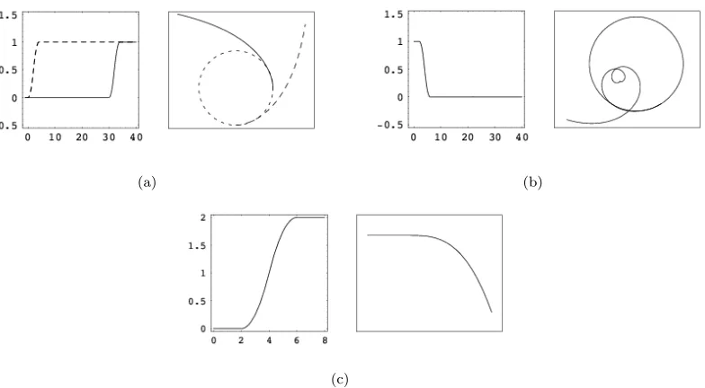
Figure 2.4: Control Primitives for Chaplygin Sleigh. (a) Transition form a circle to the trajectory with desired direction (b) Transition from a generic trajectory to a circle (c) Transition from a straight line to a generic trajectory.

If a = f(t), the system’s trajectory leaves the circle along the dashed curve in Figure 2.4 (a). The trajectory corresponding to a = a(t) = f(t ₋30) is the solid curve in Figure 2.4 (a).

Figure 2.4 (b) illustrates the control input that steers the system from a generic trajectory to a circular one. The initial value ofais 1, anda(t) is set to 1₋F1,4(t−2).

Figure 2.4 (c) illustrates the transfer from a straight line to a generic trajectory. The initial value of a is 0.1 andb(t) equals F2,4(t).

2.5 Conclusions

In this chapter we have developed a dynamical system approach to controlling the asymptotic dynamics of the Chaplygin sleigh. The key feature of our algorithm is the use of the controlled dynamics only for switching to and from circular trajectories. As a consequence, the controller remains unpowered most of the time.

(47)

(48)

Chapter 3 Geodesic Based

Proportional–Derivative (PD)

Control on Riemannian Manifolds

In this chapter a geodesic-based formulation of geometric PD tracking control for fully actuated mechanical systems is derived from the Riemannian metric. The re-gion of stability is determined directly from the size of the injectivity radius and, for a restricted set of control problems, the locus of cut points about a desired ref-erence point in the manifold. Exponential stability is proven for controlled motion along a geodesic, yielding a particularly simple, yet elegant, methodology for control design. This chapter concludes with the geometry of the double gimbal system, a particular mechanical system on which the geodesic–based, PD control design can be implemented.

3.1 Introduction

The applicability of differential geometry and topology to the discipline of theoretical mechanics has been clear for some time [1]. Hence it is not a surprising development for one to conceive the notion that a more complete understanding of the control of

(49)

mechanical systems, or simply, machines, may also reside within these frameworks. It so happens that many recent advances in control theory were obtained using the machinery of differential geometry and topology. Specifically regarding the theory of control design, it has clearly been demonstrated ( [9, 10, 8] ) that Riemannian geometry can be utilized to naturally approach a variety of control design problems and to obtain a proper perspective on commonly used control logic. Of particular interest to us is the notion of the geodesic spring introduced by Bullo, Murray, and Sarti in [9]. We expound upon this idea as it is the foundation of the control approach we shall take up herein.

Essentially, the philosophy of control system design is to create in the closed loop a well understood mechanical analogy. In more cases than not, the mass–spring– damper or the proportional derivative (PD) system is that to which the analogue system is compared. This is fitting, as its one of the few systems we understand quite well. The awkward part of this philosophy, in the context of mechanical systems, is the manner in which it is most often realized. By and large, typical control designs are brought to fruition and their subsequent analyses are carried out in Rn_{. In some} sense working in Rn _{is quite a natural thing to do and is easy enough to fall into;} for it is typical to measure by some means the states of the physical system at hand, which then, either directly or indirectly, provide ordinates orn-tuples of real numbers from which a controls engineer elicits an input command. However, the configuration manifolds of ideal machines are typically not Rn_{. As a result, the intrinsic nature of} the machines one desires to understand and control is disregarded in typical control design.

In [9] a geodesic based, PD, set–point controller was introduced and “imple-mented” on the two-sphere. In the conclusions of this paper it was stated that the geometric design of controllers for tracking on, not only the sphere and Lie groups, but also a general Riemannian manifold, was a problem of future interest.

(50)

the tracking problem on an arbitrary Riemannian manifold. This platform was hinged upon two mappings that generalized the notions of configuration error and velocity error. The latter object is constructed by means of a transport map that is “compat-ible” with the configuration error mapping. It should be emphasized that to actually specify the controller of [10] for specific machines requires the explicit presentation of both the configuration error and compatible transport mappings. Utilizing the alge-braic structure of a Lie group, Bullo and Murray were able to construct a compatible pair and thus able to employ their controller on systems which evolve on SO(3) and SE(3).

Since the geodesic spring paradigm of [9] appears to have been the impetus for [10], it seems natural and highly desirable to return to an intrinsic geometric setting for tracking on Riemannian manifolds. Indeed, that is the purpose of this paper. That is, we are particularly interested in demonstrating herein, how a machine’s intrinsic geometry (i.e. the geometry induced by the machine’s kinetic energy tensor) can be exploited within the a generic framework similar to that of [10] in order to general-ize [9]. In the intrinsic geometry setting there is an obvious choice of configuration error and transport map. Namely, they are the quadratic function of intrinsic distance and parallel transport along geodesic paths. However, control design based upon im-plicit geometry is technically difficult due to the non-trivial nature of Riemannian geometries. Nevertheless, we show that control is feasible on an ”appropriate region” of the configuration manifold.

(51)

section, it is explicitly argued that our control approach is a geodesic mass–spring– damper. In Section 3.5 we discuss our injectivity radius assumption and provide some examples.

3.2 Background Material

3.2.1 Some Conceptual and Notational Overhead

It is presumed that the reader has a knowledge of manifolds, bundles, and associated objects. We state here the notations associated to said notions that we shall use.

Q: A smooth connected manifold. Throughout this writing we shall make reference to pairs of points taken from Q. We will consistently use r and q to denote these points.

(Uα, φα): An indexed coordinate chart compatible with the atlases comprising the

differentiable structure of Q.

qi: The ith coordinate function xi ◦φα : Q → Rn : q 7→ (q1(q), . . . , qn(q))

associated to a chart (Uα, φα).

F: If f is a mapping between manifolds, the local representation thereof.

fx(y): Iffis a function ofQ×Qor any other product, then we use this convention

to denote the restriction f(x, y)_|xfixed. Similarly, fy(x)

∆

=f(x, y)_|yfixed.

TqQ: The tangent space toQ at the pointq ∈Q.

(52)

T∗

qQ: The cotangent space to Q at the point q∈Q.

ωq: An element of Tq∗Q.

(E, π, M): A fibre bundle with total space E, base space M, and projection π. We will often refer to the bundle by the total space.

T Q: The tangent bundle of Q.

v: An element ofT Q.

qi, vj: The coordinate functions associated to a chart (Uα, φα) ofT Qthat reflects

a local trivialization this bundle.

(~q, ~v) If we desire to make use of coordinate vectors to describe the image of the qi and vk collectively, we will use this notation.

X(Q): The set of smooth vector fields on Q. Typical representatives of this set will be denoted X, Y, . . . ,etc. We use Yr to indicate that the field Y has

been evaluated at a particular pointr andY(r) to denote a functional de-pendence upon a variable pointr. The same conventions will be observed for tensor fields in general.

3.2.2 Basic Intrinsic Geometry

(53)

Let Qdenote a Riemannian manifold with metric tensor g. The metric structure is sufficient enough to describe a geometry on Q, for it emits the notion of lines and angles as well as length and angle measures. We will only briefly describe the lines of the geometry and the metric.

We focus first on the ruler. The restriction of a smooth curve σ : R _→ _Q _to the compact interval [a, b] shall be called a segment connecting pointsr =σ(a) and q =σ(b). Designating u as the curve “parameter” or coordinate on R_{, the length of} a segment is given by the line integral of its speed:

lσ_{(r, q) =}

Z b

a

s

g

µ

dσ du,

dσ du

¶

du .

If S(r, q) denotes the set of all segments connecting r and q then the Riemannian manifold’s intrinsic distance is defined as

dist(r, q) = inf

σ∈S(r, q)l

σ_{(r, q)}_.

The intrinsic distance of a Riemannian manifold is a metric and its induced topology corresponds to that of the configuration manifold (a quite important fact indeed).

Now let us describe the lines of the geometry. The metric structure induces the Levi-Civita or Riemannian connection _∇, which itself effects a covariant derivative

D

du of vector fields on smooth curves. This covariant derivative then identifies the zero

acceleration curves γ or the geodesics of the manifold (lines of the geometry). That is, Dγ_du′ = 0. We denote the parameterized geodesic with velocityv atu= 0 byγ(u, v) and we simply useγ(u) when the initial data is of little concern. Thus, components of the geodesic induced by a selection of chart satisfy the following second order system of ordinary differential equations (ODEs)

D du

dγk

du = d2_γk

du2 + Γ

k ij

dγi

du dγj

(54)

where Γk

ij denote the Christoffel symbols and summation over repeated indices is

implied. The classic existence and uniqueness theorems from the qualitative theory of ODEs ensures a flow box for this system.

3.2.3 The Exponential Map and Related Geometric Notions

Now we focus on the primary analytic tool associated to the Riemannian geome-tries, the exponential mapping exp : TQ_→ Q. This mapping allows us to gather the geodesic spray of points r inQ (all of the lines emanating from r) and is defined by

exp(v) =γ(1, v)

for v sufficiently small.

For a fixed r_∈Q, we also make use of the restriction exp_r: TrQ→Q. The

homo-geneity property of geodesics ensures us that, for the given point r, the exponential mapping is defined on a sufficiently small neighborhood of 0_∈ TrQ. Further, letting

Bε(0) be a ball centered at the origin of Rn of radius ε, we have

Proposition 3.2.1 Given r_∈Q, _∃ε >0_∋exp_r: Bε(0) →Q is a diffeomorphism of

Bε(0) onto an open subset of Q.

If exp_r is a diffeomorphism of a neighborhood V of the origin in TrQ, exprV = N

is called a normal neighborhood of r in Q. If Bε(0) is such that Bε(0) ⊆ V, we call

Bε(r) = exprBε(0) the normal ball (or geodesic ball) with center r and radius ε.

Using this proposition, the exponential mapping allows us to create several special charts. By selecting an ordered orthonormal basis for TrQand inducing a coordinate

system for this linear space w.r.t. this basis, we create by means of the local diffeo-mophism expr a system of coordinates on the image of the maximal normal

neighbor-hood of r. Such a system of coordinates is called a normal coordinate system. Radial lines in this coordinate system get mapped onto the image (trace) of geodesics and (lγ₎2_{(r, q) =} _q2

(55)

the same manner, defining polar coordinates on tangent space we obtain the geodesic polar coordinate system in which the arclength actually plays the role of a coordinate. Making use of these tools and other results the following proposition may be established:

Proposition 3.2.2 Let r_∈N, N a normal neighborhood of r, andB _⊆N a normal ball of center r. Let γ : [0,1] _→ B be a geodesic segment with γ(0) = r. If σ : [0,1]_→Q is any piecewise differentiable curve joining γ(0) to γ(1), then lγ _≤_lσ _and if equality holds then γ([0,1]) = σ([0,1]).

Thus, geodesics are locally minimizing curves. That is, for q in a sufficiently small neighborhood, specifically, in a normal neighborhood of a point r_∈Q,

dist(r, q) =lγ(r, q) (3.1)

where γ is the unique (arc–length parameterized) geodesic connecting r to q. In fact, as we will illustrate at a later juncture, this relation is, under conditions to be discussed, smooth. We shall utilize these facts extensively and equation (3.1) is the crux of the intrinsic view of the geodesic spring paradigm. Consequently, we have need of knowing at what point this state of affairs ceases to persist.

Of course, this relation fails if a member fails to be defined. In an incomplete manifold, γ may not extend indefinitely and the spray of r may not cover Q. In this situation the right member becomes undefined for certain q and the relation must end. Thus, it may ease one’s path to consider taking up the assumption that Q be geodesically complete. Under this assumption one may invoke the Hopf–Rinow theorem. This theorem asserts that the completeness assumption is equivalent to, amongst other things, the following:

1. exp_r is defined on all of TrQ.

2. The closed and bounded sets of Q are compact.

On Geometric Control Design for Holonomic and Nonholonomic Mechanical Systems

Biography

Acknowledgments

Table of Contents

List of Tables

List of Figures

Notation

Introduction

1.1

Selective Historical Excerpts

1.2

Literature Background and Statement of

Con-tributions

1.2.1

Short Summary of BKMM [3]

1.2.2

Short Summary of Bullo et.

al.

[9] and Bullo and

Murray [6]

1.2.3

Short Summary of LKN [28]

1.3

On the Structure of this Document

Chapter 2

The Moving Mass Chaplygin Sleigh

2.1

Introduction

2.2

The Dynamics of the Chaplygin Sleigh

2.2.1

The Configuration Variables

2.2.2

The Momentum Dynamics and Reconstruction

2.3

Controllability of the Chaplygin Sleigh with a

Moving Mass

2.3.1

The Reduced Controlled Dynamics

2.3.2

Controllability of Asymptotic Directions

2.4

Simulations

2.5

Conclusions

Chapter 3

Geodesic Based

Proportional–Derivative (PD)

Control on Riemannian Manifolds

3.1

Introduction

3.2

Background Material

3.2.1

Some Conceptual and Notational Overhead

3.2.2

Basic Intrinsic Geometry

3.2.3

The Exponential Map and Related Geometric Notions