Nonlinear Sliding Control for Nonlinear Uncertain Systems

(1)

ISSN(Online) : 2319-8753 ISSN (Print) : 2347-6710

I

nternational

J

ournal of

I

nnovative

R

esearch in

S

cience,

E

ngineering and

T

echnology

(An ISO 3297: 2007 Certified Organization)

Vol. 5, Issue 10, October 2016

Nonlinear Sliding Control for Nonlinear

Uncertain Systems

B.Shanmugam1, Dr.K.Balagrurunathan2

Professor, Dept. of EEE, ST. Peter’s University, Avadi, Chennai, India Advisor, ST. Peter’s University, Avadi, Chennai, India

ABSTRACT: This paper focuses mainly on the classical variable structure control (VSC), also known as sliding mode

control (SMC) theory briefly In section.2 the paper briefly introduces the classical principle of sliding mode control method. Standard sliding modes provide for finite-time convergence, precise keeping of the constraint and robustness with respect to internal and external disturbances. In section 3 the importance of existence of sliding mode and its stability in the sense of Lyapunov is explained. In section 4 the procedure of designing linear sliding surface for nonlinear uncertain systems are dealt to familiarize with Sliding Mode Control. In section 5 the procedure of designing nonlinear sliding surface for nonlinear uncertain systems are derived and highlighted. This drawback is high frequency oscillations which inevitably appear in any real system is usually called chattering. This is a highly undesirable phenomenon, because it causes serious wear and tear on the actuator components. Therefore, to eliminate chattering, in section 6 Boundary Layer method is proposed and explained. Conclusions are stated

KEYWORDS: Variable Structure Control, Sliding Mode Control,

I. INTRODUCTION

Variable Structure Control (VSC) or Sliding Mode Control (SMC) was proposed in the early 1950s (Utkin, 1965), (Emelyanov, 1967), (Itkis, 1976), (Utkin, 1977),(Utkin, 1978). Over the past several decades, increasing attention has been drawn to VSC or SMC and hitherto, significant approaches have been developed world widely (Young, 1977). SMC is one of the well-known robust control design methods which only require the upper bounds of the parametric uncertainties and disturbances. Due to the simplicity and superb robustness of SMC, numerous successful applications have been carried out to a wide variety of engineering systems, such as electric drives, robotic manipulators, etc (Slotine and Sastry, 1983). In terms of Filippov’s work (Filippov, 1964), (Filippov, 1988), in which the author derived a formal justification which is one possible technique for determining the system motion in a sliding mode, the properties and the definition of the sliding mode have been well presented in detail in (Utkin, 1978) and (Utkin, 1992). A standard SMC controller is designed in two stages. One is the sliding manifold or switching surface. The essential feature of the sliding mode control is the choice of a switching surface of the state space according to the desired dynamical specifications of the closed-loop system. The plant dynamics restricted to this surface or manifold represent the controlled system’s behavior. The other is the discontinuous control law which is designed to steer the trajectories onto the sliding manifold in finite time and to keep the subsequent motion on it. In the ideal case, the resulting motion is called sliding mode. The main advantages of the sliding mode control are:

The resulting systems have their insensitivities or robustness against a large class of perturbations or model uncertainties, which enter the system in the same channel as control inputs;

(2)

I

nternational

J

ournal of

I

nnovative

R

esearch in

S

cience,

E

ngineering and

T

echnology

II. SLIDING-MODE CONTROL THEORY

This work deals with a special class of systems called “variable structure systems” (VSSs). They are of great importance in systems and control theory. As described by Utkin (1977) the basic concept of VSCs is that the system is allowed to change structure at any instant. The design problem in VSCs is therefore to find the parameters in each of the system structures and to design the switching logic which decides when the structure of the system should change. One of the key features of Variable Structure Systems is that the resulting system can show properties not present in any of the separate system structures. The motion described by these trajectories is known as sliding mode.

The response of a system with sliding mode control can basically be divided into two parts

1. The reaching phase: When s ≠ 0, the system is said to be in the reaching phase. The trajectories in the phase plane will in this phase move toward the surface S.

2. The sliding phase: Once the system reaches S the trajectories will move along the surface described by S until it reaches the equilibrium point.

III. EXISTENCE OF A SLIDING MODE

Existence of a sliding mode (Itkis, 1976; Utkin, 1977, 1992; Edwards and Spurgeon, 1998) requires stability of the state trajectory to the sliding surface s (x) = σ(x) = 0 at least in a neighborhood of {x│σ(x) = 0}, i.e., the system state must approach the surface at least asymptotically. The largest such neighborhood is called the region of attraction. From a geometrical point of view, the tangent vector or time derivative of the state vector must point toward the sliding surface in the region of attraction (Itkis, 1976; Utkin,1992) (see Fig. 2.2). For a rigorous mathematical discussion of the existence of sliding modes see Itkis (1976); White and Silson (1984); Filippov(1988); Utkin (1992).

The existence problem can be seen as a generalized stability problem; hence the second method of Lyapunov provides a natural setting for analysis. Specifically, stability to the switching surface requires to choose a generalized Lyapunov function V (t; x) which is positive definite and has a negative time derivative in the region of attraction.

Theorem3.1 For the (n-m)-dimensional domain D to be the domain of a sliding mode, it is sufficient that in some n -

dimensional domain Ω ∈ D, there exists a function V (t, x, σ) continuously differentiable with respect to all of its arguments, satisfying the following conditions:

1. V (t; x; σ) is positive definite with respect to σ , i.e., V (t; x; σ) > 0, with σ ≠ 0 and arbitrary t, x, and V (t; x; 0) = 0; and on the sphere ║σ║ = ρ, for all x ∈ Ω and any t the relations:

‖ ‖ V (t, x, ) = , > 0 (3.1)

‖ ‖ V (t, x, ) = , > 0 (3.2)

hold, where h , and H , depend on ρ (h ≠ 0 if ρ ≠ 0).

2. The total time derivative of V (t, x, σ) for the system (4.1) has a negative supremum for all x ∈ Ω except for x on the switching surface where the control

inputs are undefined, and hence the derivative of V (t; x; σ) does not exist. Proof: See Utkin (1977).

The structure of the function V (t, x,σ) determines the ease with which one computes the actual feedback gains implementing a sliding mode control design. Unfortunately, there are no standard methods to find Lyapunov functions for arbitrary nonlinear systems. Note that, for all single input systems a suitable Lyapunov function is

V(x, t) = (x)

which clearly is globally positive definite. In sliding mode control, σ̇ will depend on the control and hence if switched feedback gains can be chosen so that

̇(t, x, ) = < 0 (3.3)

(3)

I

nternational

J

ournal of

I

nnovative

R

esearch in

S

cience,

E

ngineering and

T

echnology

Condition (2.7) is often replaced by the so-called η- reachability condition (Utkin, 1977, 1992; Edwards and Spurgeon, 1998)

̇(t, x. ) = <− │ │ (3.4)

which ensures finite time convergence to σ(x) = 0, since by integration of (3.4) one has

| [ ( )]|−| ( )| ≤ −

showing that the time required to reach the surface, starting from the initial condition σ[x(0)] is bounded by

= │ [ ( )]│

The feedback gains which would implement an associated sliding mode control design are straightforward to compute in this case (Utkin, 1977; Slotine and Li, 1991; Sira-Ramirez, 1992; Zinober, 1994; Edwards and Spurgeon, 1998; Young et al., 1999).

IV. LINEAR SLIDING SURFACE DESIGN

Let us consider an example to explain the steps of designing Linear Sliding Line for the control of the second-order nonlinear plant. The set of the following equations has been chosen to describe the second-order nonlinear plant: ẋ = x

ẋ = bcos(k, x ) + u

(or)ẋ = f(x , x , t) + u (4.1) with initial conditions, x (0) = x and x (0) = x

where |b| < 1, k > 0 are the constant parameters of the plant, x1, x2 are state variables (error and its derivative)

and u is the control signal and the disturbance term f (x1, x2, t) = ( , ) , which may comprise dry and

viscous friction as well as any other unknown resistance forces, is assumed to be bounded, i.e.,

| ( , , )| ≤ L > 0 .

The problem is to design a feedback control law u = u (x1, x2) that drives the mass to the origin asymptotically. In other

words, the control u = u (x1, x2) is supposed to drive the state variables to zero: i.e., →∞ , = 0 and the definition

of the sliding surface which is the track to be mapped by the system trajectory while converging towards the origin. In case of the considered second-order plant the switching surface is reduced to the switching line and defined by the differential equation (4.2):

s = c + ̇ (4.2) where c is the positive constant slope of the switching line s = 0. Then the control signal u is assumed as shown in the equation (4.3):

Since ( ) = ̇ ( ), a general solution of Eq. (4.2) and its derivative is given by

( ) = (0) (− )

( ) = ̇ =− (0) (− ) (4.3)

both ( ) and ( ) converge to zero asymptotically. Note, no effect of the disturbance

f (x1, x2, t) on the state compensated dynamics is observed. How these compensated dynamics could be achieved? First,

we introduce a new variable in the state space of the system in Eq. (4.1):

= ( , ) = + , c > 0 (4.4)

In order to achieve asymptotic convergence of the state variables x1, x2 to zero, i.e., →∞ , = 0 with a given

convergence rate as in Eq. (4.3), in the presence of the bounded disturbance

f (x1, x2, t), we have to drive the variable s in Eq. (4.4) to zero in finite time by means of the control u. This task can be

achieved by applying Lyapunov function techniques to the s -dynamics that are derived using Eqs. (4.1) and (4.4):

̇= + ( , , ) + , ( ) = (4.5)

For the s - dynamics (4.5) a candidate Lyapunov function is introduced taking the form

V = (4.6)

In order to provide the asymptotic stability of Eq. (4.5) about the equilibrium point = 0, the following conditions must be satisfied:

(4)

I

nternational

J

ournal of

I

nnovative

R

esearch in

S

cience,

E

ngineering and

T

echnology

(b) | |→∞ = ∞

Condition (b) is obviously satisfied by V in Eq. (4.6). In order to achieve finite-time convergence (global finite-time stability), condition (a) can be modified to be

̇ = ̇ ≤ − , > 0 (4.7)

Indeed, separating variables and integrating inequality (4.7) over the time interval 0 ≤ ≤ , we obtain

( )≤ − + ( ) (4.8)

Consequently, V (t) reaches zero in a finite time tr that is bounded by

≤ ( ) (4.9)

Therefore, a control u that is computed to satisfy Eq. (4.7) will drive the variable s to zero in finite time and will keep it at zero thereafter. The derivative of V is computed as

̇ ₌_̇₌ ₍ ₊ ( , , ) +

(4.10) Assuming u =− + v and substituting it into Eq. (4.10) we obtain

̇ = s ( ( , , ) + ) = s ( , , ) + ≤ | | + (4.11)

Selecting v =− sign (s) where

sign (s) =

−

> 0

< 0 (4.12)

and sign (0) ∈[−1, 1] (4.13) with > 0 and substituting it into Eq. (4.11) we obtain

̇ ≤ | | + | | =−| |( − ) (4.14)

Taking into account Eq. (4.5), condition (4.7) can be rewritten as

̇ ≤ − = ̇= −

√ | | > 0

(4.15) Combining Esq. (4.14) and (4.15) we obtain

̇ ≤ −| |( − ) =−

√ | | (4.16)

Finally, the control gain is computed as = +

√ (4.17)

Consequently a control law u that drives to zero in finite time (2.28) is

u = − − ( ) (4.18)

Remark 2.1. It is obvious that ̇ must be a function of control u in order to successfully design the controller in Eq.

(4.7) or (4.18). This observation must be taken into account while designing the variable given in Eq. (4.4).

Remark 2.2. The first component of the control gain Eq. (4.17) is designed to compensate for the bounded disturbance

f (x1, x2, t) while the second term

√ is responsible for determining the sliding surface reaching time given by Eq. (4.9).

The larger is the , the shorter, the reaching time.

Now it is time to make definitions that interpret the variable (4.4), the desired compensated dynamics (4.1), and the control function (4.18) in a new paradigm.

Definition 1.1. The variable (4.4) is called a sliding variable

Definition 1.2. Equations (4.1) and (4.4) rewritten in a form:

(5)

I

nternational

J

ournal of

I

nnovative

R

esearch in

S

cience,

E

ngineering and

T

echnology

corresponds to a straight line in the state space of the system (4.1) and are referred to as a sliding surface. Condition (4.7) is equivalent to s ̇ ≤ −

√ | | and is often termed the reachability condition. Meeting the reachability or

existence condition (4.7) means that the trajectory of the system in Eq. (4.1) is driven towards the sliding surface (4.2) and remains on it thereafter.

Definition 1.3. The control u = u (x1, x2) in Eq. (4.18) that drives the state variables x1, x2 to the sliding surface

(4.4) in finite time , and keeps them on the surface thereafter in the presence of the bounded disturbance f (x1, x2, t), is called a sliding mode controller and an ideal sliding mode is said to be taking place in the system

(4.1) for all t > tr (ref Fig 2.2) .

Fig.2.2. Real Sliding-Mode Control with chattering of the plant described by (4.1)

V. NONLINEAR SLIDING SURFACE DESIGN

Filippov's method is one possible technique for determining the system motion in sliding mode as outlined in the previous section. In particular, computation of represents the "average" velocity ̇ of the state trajectory restricted to the switching surface. A more straightforward technique easily applicable to multi-input systems is the equivalent control method, as proposed in Utkin (1977, 1992) and in Drazenovic (1969).

It has been proved that the equivalent control method produces the same solution of the Filippov method if the controlled system is affine in the control input while the two solutions may differ in more general cases.

The method of equivalent control can be used to determine the system motion restricted to the switching surface (x) = 0. The analytical nature of this method makes it a powerful tool for both analysis and design purposes.

Let a single input nonlinear system be defined as

̇ = f (x,t) + b(x,t) u(t) (5.1)

Here, x (t) is the state vector of order n, u(t) is the control input and x is the output state of the interest. The other states in the state vector are the higher order derivatives of x up to the (n-1)-th order. f ( x ,t) and b ( x ,t) are generally nonlinear functions of time and states. The function f (x) is not exactly known, but the extent of the imprecision on f (x) is upper bounded by a known, continuous function of x.

The control problem is to get the state x to track a specific time-varying state in the presence of model imprecision on f (x) and b (x). A time varying surface s (t) is defined in the state space R(n) by equating the variable s (x; t) , defined below, to zero.

s (x, t) = ( + )n-1 (t) (5.2)

(6)

I

nternational

J

ournal of

I

nnovative

R

esearch in

S

cience,

E

ngineering and

T

echnology

we only need to differentiate s once for the input u to appear. Furthermore, bounds on s can be directly translated into bounds on the tracking error vector , and therefore the scalar s represents a true measure of tracking performance. The corresponding transformations of performance measures assuming (0) =0 is:

∀ t ≥ 0, │s (t)│≤ ⇒ ∀ t ≥0,

│ (i)(t) │≤(2 ) i =0... n-1 (5.3)

where = / (Slotine and Li 1990 ). In this way, an n-th-order tracking problem can be replaced by a 1st-order stabilization problem.

The simplified, 1st-order problem of keeping the scalar s at zero can now be achieved by choosing the control law u of (5.1) such that outside of S(t)

= − │ │ (5.4)

where is a strictly positive constant. Condition (5.4) states that the squared “distance” to the surface, as measured by s2, decreases along all system trajectories. Thus, it constrains trajectories to point towards the surface s(t). In particular, once on the surface, the system trajectories remain on the surface. In other words, satisfying this sliding condition makes the surface an invariant set (a set for which any

trajectory starting from an initial condition within the set remains in the set for all future and past times). Furthermore (5.4) also implies that some disturbances or dynamic uncertainties can be tolerated while still keeping the surface an invariant set.

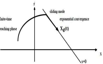
Figure 5.1: Graphical interpretation of equations (5.2) and (5.4) (n=2)

Finally, satisfying (5.2) guarantees that if x (t=0) is actually off (t=0), the surface S(t) will be reached in a finite time smaller than │s (t = 0)│ / . Assume for instance that s (t=0) > 0, and let be the time required to hit the surface s = 0. Integrating (5.4) between t=0 and leads to

[0 – s (t = 0)] = [s (t = ) – s (t=0)] ≤ - η (t -0) which implies that

t ≤ ( )

The similar result starting with s(t=0) > 0 can be obtained as t ≤| ( )|

Starting from any initial condition, the state trajectory reaches the time-varying surface in a finite time smaller than

| ( )|

, and then slides along the surface towards x (t) exponentially, with a time-constant equal to 1 / η .

(7)

I

nternational

J

ournal of

I

nnovative

R

esearch in

S

cience,

E

ngineering and

T

echnology

VI. CONTROLLER DESIGN

The controller design procedure consists of two steps. First, a feedback control law u is selected to verify sliding condition (5.4). However, in order to account for the presence of modeling imprecision and of disturbances, the control law has to be discontinuous across s (t). Since the implementation of the associated control switching is imperfect, this leads to chattering (see figure 5.2), chattering is undesirable in practice, since it involves high control activity and may excite high frequency dynamics neglected in the course of modeling. Thus, in a second step, the discontinuous control law u is suitably smoothed to achieve an optimal trade-off between control bandwidth and tracking precision. The first step achieves robustness for parametric uncertainty; the second step achieves robustness to high frequency unmodeled dynamics. This section discusses the first step.

Consider a simple second order system

ẍ(t) = f (x, t) + u (t) (5.5)

where f (x, t) is generally nonlinear and/or time varying and is estimated as f( x , t ), u(t) is the control input, and x(t) is the state to be controlled so that it follows a desired trajectory x ( t ) . The estimation error on f(x, t) is assumed to be bounded by some known function F = F(x, t), so that

│ (x, t) – f(x, t) │ ≤ F(x, t) (5.6)

we define a sliding variable according to (5.2)

s (t) = ( + ) (t) = ̇(t) + (t) (5.7)

Differentiation of the sliding variable yields

ṡ(t) = ẍ(t) - ẍd (t) + γẋ(t) (5.8)

Substituting Equation (4.5) in Equation (4.8), we have ̇(t) = f (x, t) + u (t) - ̈d (t) + ̇(t)

(5.9) The approximation of control law u(t) to achieve ṡ(t) = 0 is

(t) = (x, t) + ̈d (t) - ̇(t)

(5.10)

u (t) can interpreted as the best estimate of the equivalent control.

To account for the uncertainty in f (x, t) while satisfying the sliding condition

( ( ) ) ≤− │ ( )│, >0 (5.11)

take the control law as:

u(t) = u(t) – k(x, t) sign(s(t)) (5.12) By choosing k(x, t) large enough, such as

k (x, t ) F(x ,t )

ensures the satisfaction of condition (5.11), since

( ( ) ) = ̇(t) s (t) = (f(x, t) - (x, ))

s(t) – K(x, t)│s (t)│ ≤ − │ ( )│

(5.13)

Hence, by using (5.12), we ensure the system trajectory will take finite time to reach the surface s (t), after which the errors will exponentially go to zero.

From this basic example, we can see the main advantages of transforming the original tracking problem into a simple 1st-order stabilization problem in s.

Now consider the second order system in the form of

̈(t) = f (x, t) + b(x, t) u(t ) (5.14)

where b(x, t) is bounded as 0 ≤b (x, t) ≤ b(x, t) ≤b (x, t)

The control gain b(x, t) and its bound can be time varying or state dependent. Since the control input is multiplied by the control gain in the dynamics, the geometric mean of the lower and upper bound of the gain is a reasonable estimate: b(x, t) = b (x, t)b (x, t)

(8)

I

nternational

J

ournal of

I

nnovative

R

esearch in

S

cience,

E

ngineering and

T

echnology

β ≤ ≤β , where β = (β /β )1/2

since the control law will be designed to be robust to the bounded multiplicative uncertainty,

is called the gain margin of the design.

It can be proved that the control law

u (t) = ( , ) [ (t) – k(x, t)sign(s(t))]

(5.15) with

k (x, t ) ( x, t)( F( x, t) ) ((x, t ) 1)│ ( )│

satisfies the sliding condition.

The control law for higher order system can be deducted based on similar approach

VII. CHATTERING REDUCTION

An ideal sliding mode exists only when the state trajectory x (t) of the controlled plant agrees with the desired trajectory on s(x) = σ(x) = 0 at every t t1 for some t1 . This may require infinitely fast switching. In real systems, a switched controller has imperfections which limit switching to a finite frequency. The representative point then oscillates within a neighborhood of the switching surface. This oscillation, called chattering, is illustrated on figure 5.2.

Figure 5.2: Chattering as a result of imperfect control switching (Resource: Slotine and Li 1991)

Control laws which satisfying sliding condition (5.4) and lead to “perfect” tracking in the face of model uncertainty, are discontinuous across the surface s (t), thus causing control chattering. Chattering is undesirable, since it involves extremely high control activity, and furthermore may excite high-frequency dynamics neglected in the course of modeling. Chattering must be reduced (eliminated) for the controller to perform properly. This can be achieved by smoothing out the control discontinuity in a thin boundary layer neighboring the switching surface

B (t ) = {x,│ s( x; t)│≤ } > 0 (5.16)

where is the boundary layer thickness, and



(Ref. Eqn.5.3) is the boundary layer width. In other words,

outside of B(t), we choose control law as before which guarantees that the boundary layer is attractive, hence invariant; all trajectories starting inside B(t=0) remain inside B(t) for all t 0 ; and then u is interpolated inside B(t). For example, sign(s) in (5.12) can be replaced by s / ϕ inside B (t).

This approach leads to tracking to within a guaranteed precision (rather than perfect tracking), and more generally

guarantees that for all trajectories starting inside B(t=0)

t 0,│ ( )( )│( ) i=0.. n-1 (5.17)

VIII. CONCLUSION

Due to its robustness properties, sliding mode controller can solve two major design difficulties involved in the design of a braking control algorithm:

(9)

I

nternational

J

ournal of

I

nnovative

R

esearch in

S

cience,

E

ngineering and

T

echnology

2. the performance of the system depends strongly on the knowledge of the tire/road surface condition;

For the class of systems to which it applies, sliding controller design provides a systematic approach to the problem of maintaining stability and consistent performance in the face of modeling imprecision.

REFERENCES

1.A. Levant. Sliding mode control. International Journal of Control, 58(6):1247–1263, 1993.

2. Slotine J. J. E., “Sliding controller design for nonlinear systems”, International Journal of Control, Vol. 40, pp. 421-434, 1984.

3. A. J. Fossard T. Floquet. Sliding Mode Control in Engineering, chapter Introduction: An Overview of Classical Sliding Mode Control, pages 1–27. Marcel Dekker, Inc., 2002

4.S.V.Emelyanov,.BinaryAutomatic Control Systems, Translated from the Russian, Mir Pub. 1987

5. V.I.Utkin, Sliding modes and their application in variable structure systems, Translated from the Russian Mir Pub. 1978, 4.Bartolini, D.; Ferrara, A. & Usai, E. (1998). Chattering avoidance by second-order sliding

mode control. IEEE Trans. on Automatic Contr. Vol., 43, 241–246

5.DeCarlo, R S.; Żak S. & Mathews G. (1988). Variable structure control of nonlinearmultivariable systems: a tutorial. Proceedings of the IEEE. Vol., 76, 212–232

6.Edwards C. & Spurgeon, S. K. (1998). Sliding mode control: theory and applications. Taylor and Francis Eds

7.Hung, J. Y.; Gao W. & Hung, J. C. (1993). Variable structure control: a survey. IEEE Trans. On Ind. Electron. Vol., 40, 2–22 8.Levant, A. (1993).Sliding order and sliding accuracy in sliding mode control. Int. J. of Contr. Vol., 58, 1247–1263

9.Utkin, V. & Shi, J. (1996). Integral sliding mode in systems operating under uncertainty 10.B.Shanmugam, Dr.K.Balagrurunathan, Sliding mode theory and application