A building block model for quantitative genetics.

(1)

Copyright 0 1989 by the Genetics Society of America

A

Building Block Model

for

Quantitative Genetics

Hidenori Tachida and C. Clark Cockerham

Department of Statistics, North Carolina State University, Raleigh, North Carolina 27695-8203

Manuscript received July 16, 1988 Accepted for publication December 6, 1988

ABSTRACT

We introduce a quantitative genetic model for multiple alleles which permits the parameterization of the degree, 8, of dominance of favorable or unfavorable alleles. We assume gene effects to be random from some distribution and independent of the 9 ' s . We then fit the usual least-squares population genetic model of additive and dominance effects in an infinite equilibrium population to

determine the five genetic components-additive variance uf, dominance variance uz, variance of homozygous dominance effects d2, covartance of additive and homozygous dominance effects d l , and the square of the inbreeding depression h-required to treat finite populations and large populations that have been through a bottleneck or in which

-

there is inbreeding. The effects of dominance can be summarized as functions of the average, 8, and the variance, a&. An important distinction arises between symmetrical and nonsymmetrical distributions of gene effects. With symmetrical distributions d l = -d2/2 which is always negative, and the contribution of dominance to uz is equal to d2/2. With nonsymmetrical distributions there is an additional contribution X to uz and - X / 2 to d l , the sign of X being determined by and the skew of the distribution. Some numerical evaluations are presented for the normal and exponential distributions of gene effects, illustrating the effects of the number of alleles and of the variation in allelic frequencies. Random additive by additive (a*a) epistatic effects contribute to uf and to the a*a variance, &, the relative contributions depending on the number of alleles and the variation in allelic frequencies. There are plausible situations where the contribution

to a: can be larger than that to

&.

When the number of alleles is large and there is little variation in allelic frequencies most of the variance is u&. The effects of the genetic components on the additive variance within finite populations are discussed briefly.

T

0 facilitate t h e analysis of quantitative variation for a single locus in finite populations with drift (COCKERHAM 1984) and with drift, migration and extinction (TACHIDA and COCKERHAM 1987), it is necessary to define five genetic components. The same is true for large populations that have been

through a bottleneck or large populations when there is inbreeding (COCKERHAM a n d MATZINGER 1985) or partial inbreeding (WRIGHT and COCKERHAM 1985).

Defined for an infinite random mating population, these five components-additive variance, a:; dominance variance, u:; covariance of additive and homozygous dominance effects, d l ; variance of homozygous dominance effects, dB; square of the inbreeding

depression, i-were first given by HARRIS (1964). T h e total variance in the infinite population is a:

+

CT;,

but the other three components are required to treat the quantitative variation within finite populations or with inbreeding. While the five components suffice to accommodate multiple alleles with general allele frequencies and a general model of additive and dominance effects, the complexities of the compo-

nents are not easily deciphered, and practically noth- ing is known about the size of some of the components in natural or domesticated populations. O n e particu- larly bothersome component is dl which can be negative. Even with just two alleles, the number of genetic

Genetics 121: 839-844 (April, 1989)

components is reduced only to four except in the very restrictive situation of two equally frequent alleles, when there are just the additive and dominance variance components.

With only two alleles it is easy to quantify dominance in terms of dominance or partial dominance of the favorable or unfavorable allele. With multiple alleles there is a dominance parameter for each pair

of alleles and no model appears to have been published which allows us t o speak of the average degree of

dominance or of the variation in dominance.

We introduce a model which has these features and utilize it to analyze the effects of number of alleles, variation in allele frequencies, average dominance and variance of dominance on the five genetic components. We augment the model to include additive by additive ( a * a ) effects to study the effects of number of alleles and variance among allele frequencies o n the additive and (a*a) variances. Effects in each cate- gory are assumed to be randomly drawn from some

distribution and to be independent between categories and independent of gene frequencies.

MODELS A N D VARIANCES

We express the genotypic value, G , of a n individual for a particular locus with alleles A, a n d A, as

G . . = X , + X - + g . . Y . .

(2)

where Y,, =

q,

=

1 X,

-

Xj

I,

and call this the biological building block or 58 model. Dominance is portrayed by 9: no dominance, 9 = 0; dominance of the larger X , 9 = 1 ; dominance of the smaller X, 9 = -1, and so on. I n any case Gii = 2X,. T h e x’s and 9 ’ s in the 39

model represent the biological effects of the genes and genotypes on phenotype as would be determined by classical genetic experiments. These effects do not vary among populations. The main feature here is that we have extended the two-allele model to include multiple alleles and maintained the classical interpretation of dominance. T h e two-allele model further simplifies because we can orient X1

>

X 2

G I I G I , G 2 2

G i - XI - X2

x,

-

x,

9JI2(XI - X,) -(X1 - X,)

u = X ] - X ? , U au -U

= a

which can be manipulated into the model of COM-

STOCK and ROBINSON (1948) by subtracting out the mean of the two homozygotes, and 9 and a have the same dominance interpretation. With multiple alleles the orientation of the X’s is taken care of by absolute differences.

We now consider the usual least-squares model of gene effects for an infinite population in Hardy-Wein- berg equilibrium with arbitrary gene frequencies,

PI

for the ith allele, and call this the population, or

9

model

where p is the mean, a denotes an additive effect and d is the dominance effect. T h e mean and effects in this model are population specific, dependent upon gene frequencies. T h e a’s are average effects in the population such that the variance of the remainders, d’s, is a minimum. This is the correct framework for expressing the covariances of relatives, studying the effects of gene frequencies and interpreting the effects of selection.

T o relate the two models, the mean and effects in the 9 m o d e l are expressed in terms of those for the

.@ model

/A = PkP/Gk/ = 2 P k X k i- P k P l ~ k l Y k l

k l k k#/

a, =

c

p/c,

-

II = Xt

-

pix,

+

C

P@tlYiI

/ 1 I f 1

-

cc

p k p @ k / Y k l k#/

d . . II = G . . ‘I

-

a;

-

~j

-

p = 9qY,,

-

p 1 9 i / Y t l - p/9JlY,/

/#r

+

cc

f l k f l l 9 k l Y k l k#/

d,, = G,, - 2 U , - p = - 2

2 p@1/Y2/

+

cc

pkp@k[Yk/.

/#I k#/

Note that we have taken account of the fact that all

Yii

=

0.

We next formulate various quantitative genetic components for the 9 model in the usual manner

(COCKERHAM 1984) and take their expectations, de- noted by

%

as a means of defining these parametric components: additive variance, a: = 2

%‘ei

pia:; dominance variance, a; =

gcicj

pipjd:; covariance of ai

and dl*, dl =

%’Xi

p,a,di,; variance of d,,’s, dB =

%e,

p,d:

-

[59(cI

p,dil)]*; inbreeding depression, h =

%’ei

P,diz; and

k

= W(Ci pldIi)’. Ordinarily, the components are defined with the omission of the expectations. However, we want to study the effects of parameters for the Bmodel, with specific distributions of X’s and 9 ’ s , on the parametric components of the P m o d e l , which is accomplished by taking expectations.

We assume the X ’ s to be random from some distribution with mean zero and variance a:. N o generality is lost by assuming a mean of zero and a: is just an arbitrary scalar. The shape of the distribution is important. In the following expectations, different sub- scripts denote distinct alleles. L9Xp = ,:a 59Yg =

&

a,, %‘Xiye = va:, g Y q Y , k = wa:, and gY,,Ykl = aa:. The

parameters a , v and w depend on the distribution of

X . When the distribution of X is symmetrical, v = 0. If the distribution of X is normal, a = 4/7r = 1.27 and

w = 1/3

+

2 h / 7 r = 1.44, while if the distribution is uniform a = 4/3 = 1.33 and w = 1.4. For the exponential distribution,f(X) = a,’ exp[-a;’(X

+

a,)], X

2

-

ax, LY = 1, u = 0.5, w = 413 = 1.33. There are no appreciable differences among the distributions for w ,

small differences for cx but of course major differences between symmetry and nonsymmetry.

We consider the 9 s to be random variables with mean

9

and variance a$ and the values of

3

and a$

to be at our disposal for study. However, since we are generally concerned with 9 in the range (- 1, l), a

3

of 1 or -1 would imply a& = 0 and there can be an increase in

u&

as

3

approaches 0. In terms of expectations 2?9,j =

3

and 99; =

g2

+

a&. We further assume the 9 s to be independent of the X’s and both to be independent of the gene frequencies.

A shorthand notation for moments of gene frequencies is useful, q, =

p.i

( j = 2, 3, 4). With these functions and the above expectations the various genetic components for the 9 model can be expressed in terms of the moments of the X and B variables. For example, the inbreeding depression, h =

%‘El

P,d,, =

-!&9cC1z1

prp1911YII

= -(1 - q 2 ) 3

&

ax since the

p,

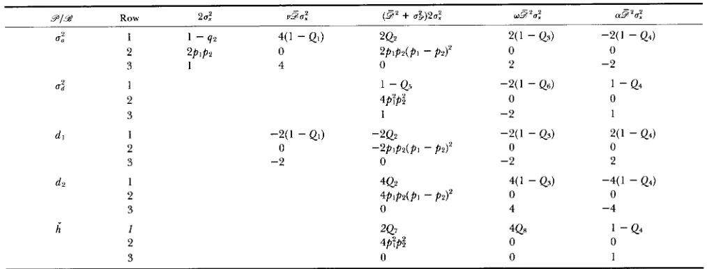
9 and Y values are independent. I n Table 1 the genetic components of the 9 m o d e l are expressed as functions of components for the 9 model, in row 1 for number of alleles and gene frequencies general, in row 2 for two alleles and in row 3 for an infinite number of alleles. For example, in Table 1 , af (row

A n alternative expression for 4 2 , q 2 = (1

+

c 2 ) / k ,

where c is the coefficient of variation of the p’s and

k

(3)

Building Block Model

TABLE 1

Coefficients of components for model g i n genetic components for model 9

84 1

U2 1

2 3

d l 1

2 3

de 1

2

3

i I

2

3

-2(1 - 41)

0

-2

2Q7

4p:p;

0

4% 1 - Q 4

0 0

0 1

Row 1 -in terms of q2 and Q's for gene frequencies general. Row 2"in terms of gene frequencies, PI and p 2 , for two alleles. Row 3"in

terms of integers for an infinite allele model. Definitions of Q's:

41

= 3q2 - 2qs; Q2 = q*

-

2qz - qs

+

2q4; Q3 = 7qp

-

4q% - 1093

+

894; Q4 = 6qn

-

3g': - 8q3

+

6q4; @ = 3q2

-

2q%

-

2qs

+

294; Q 6 = 5q2

-

2q2

-

6 q s

+

4q4; e7= q? - 44; @ = 4 2

-

4% - 2qs

+

2q4.

is the number of alleles, has previously been found useful (COCKERHAM and TACHIDA 1987). Then the coefficient 1

-

q 2 in Table 1 can be seen to decrease

as c increases and to increase as the number of alleles increases, being one for k infinite with some restriction on c. Unfortunately, the evaluation of the Q's in Table 1 is complex except for the cases of two or an infinite number of alleles. For an infinite number of alleles, all q's and consequently all Q's are taken to be zero.

With two alleles, only two components, 2a: and

(g2

+

&)2a,2, of the @model are involved since there is only one 9 , Y u term. In this case

3 ' +

a& represents the average value of 9; for a pair of alleles. Also,

note for 2 alleles that the distribution of X is immaterial as long as u: is finite. In terms of c the translation of the coefficients is 2p1p2 = (1

-

c2)/2 and 4 p l p 2 ( p l

-

p2)' = c'(1

-

c'). The term c'( 1

-

c') has a maximum

of 1 /4 when c 2 = 1/2 for gene frequencies (2 f &)/

4.

There is considerable simplification for an infinite number of alleles, when all the q's are zero, as shown in Table 1. Except for a few peculiarities we have the coefficients bounded by the values for 2 and a~ alleles, with a monotonic change from one to the other. Exceptions can be seen by considering all k alleles to have equal frequencies. For this situation q2 = k - ' , q3

= k-', q4 = and letting

hi

= k

-

i, 1

-

q2 = klk", 1

-

Ql = klk2k-', = Q~ = klk2k-3, I

-

Q~ =

klk2k4k-3,

1

-

Q~ = K M ~ K - ~ , 1

-

Q~ = k l ( k 2 k

+

2)k-3, 1

-

Q~ =

k l k ; K 3 and Q 7 = k l k P 3 . Then, 1

-

Qs for example is zero for k = 2 , negative for k = 3, zero for k = 4 and for higher k increases monotonically to one.

T h e number of alleles also affects the variance of

means. For example,

h'

=

8(Ct

pi&,)'

and h = 8

Cr pi&,.

With two alleles there is only one 9v and

L@$

=

z2

+

&.

Consequently,

i

=

4p:pz(Z2

+

a&)2a: repre-

senting the results as an average for pairs of alleles. With the infinite allele model, the mean as an average over the infinite number of alleles has no variance and

It should be stressed that the total variance in the infinite random mating population is simply af

+

CT;.

T h e three additional components are required to express the variance and covariances of relatives when there is drift and inbreeding.

We next extend the @model to include additive by additive ( m a ) effects for two loci. T h e genotypic value is now indexed in addition for alleles B k and Bl at the

second locus

i

= (8h)' = a z 2 u ; .

Gjj,,l =

x,

+

xj

+

LajjYjj

+

x;

+

x ;

+

9 ; , Y b

+

z;,

+

zi,

+

zj,

+

Zjl.

T h e primed values for the B locus have the same characteristics of independence as for the A locus but may be from different distributions with different variances. For simplicity we show only the new terms by making use of the "includes" sign 3

Gjj.,i 3 Z i k

+

Z i l

+

zj,

+

Z j l .

T h e Z's represent joint effects of pairs of A and B genes in this 53' model. We assume the Z's to be independently distributed with mean zero and variance a: and that the Z ' s are independent of the X ' s and 9 ' s for each locus.

In our population,

9

model we write the a*a effects as

Glj,kl 3 (aa)ik

+

(aa)il

+

(aa)jh

+

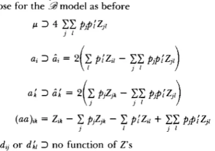
(aa)$.

(4)

We next express effects in the 9 m o d e l in terms of those for the

B

model as before

P 3 4

cc

pjpEzJ1

j l

1

d,, or d ; 3 no function of 2's

where primes are used to denote frequencies or effects at the B locus and 6's denote the a*a function of the 2's in the additive effects. We evaluate these functions in terms of expectations as before.

Cipi6,

= 0 , C k

pi6L

= 0 ,

Xi

C k pipi(aa)ik = 0 , get

pi6:

= 4 c k @;)'(I

-

Ci

p : ) d

= 4q;(l

-

q 2 ) d , 9 C k

PL(6i)*

= 4q2(1

-

qG)az, 2 d u = g x i C k ptp;(aa)t = (1

-

Ci

p? -

C k

(pi)*

+

cz

p f

C k ( p i ) 2 ) a I = ( 1

-

q2)(1

-

q 6 ) d . There are

two additive effects at each locus with the same variance and four a*a effects with the same variance, so that ai 3 8q;(l

-

q2)a:, ai, 3 8q2(1

-

q4)a: and a& =

4a& = 4( 1

-

q 2 ) ( 1

-

q;)az. In the total additive

variance, ai

+

a:,, the contribution of a*a effects is S ( q 2

+

q.i

-

2q2q;)a:. The contribution decreases with more alleles and is zero for infinite alleles at both loci. In contrast a& generally increases with the number of alleles and is :;4 with infinite alleles at both loci.

NUMERICAL ANALYSIS

On the surface we appear to have gained little by introducing the B model of biological effects for a single locus since it contains five components and there are five components for the 9 m o d e l of genetic effects with a fairly complicated translation from one set of components to the other (Table 1). The number of components for the Bmodel reduces to four when the X ' s are symmetrically distributed. In this case the contribution of dominance to the genetic components involves

3'

and a&. Some of the genetic components are now functionally related. Since d2 is the variance among homozygous dominance effects, dB 2 0 and is

a monotonically increasing function of both

3'

and

a&. From the general formulations in Table 1 we see

that d l = - d 2 / 2 and that

if

-

V , = d 2 / 2 where V , is the additive variance without dominance. Conse- quently, d l is negative, d l I 0, for symmetrical distri-

butions of allelic effects. Some numerical evaluations will illustrate these and other features.

Coefficients of a: for the genetic components are evaluated numerically for various numbers of alleles and gene frequencies in conjunction with two combinations of

3

and a& in Table 2 with X normally distributed. We chose case 1:

3

= 0, a& = 1/3,

representing a uniform distribution of 9 between the limits ( - 1 , 1 ) to illustrate the effects of variation in 9,

and case 2 :

3

= 1, a& = 0, representing complete dominance of the favorable allele, to illustrate the effects of dominance. In case 2 the results are the same for

3

= -1. Also in this case the results for any

31

other than 1 or -1 are readily found by multiply- ing the coefficients for all genetic components except

ai by 9:.

A comparison of case 1 with case 2 , shown in Table 2 , is somewhat arbitrary because

3

can be adjusted to make the two cases similar except for

h'.

It appears, however, that

3

can have considerably larger effects than a$ on the components involving dominance. With

9

= 0 there is no inbreeding depression and

h'

is generally of no consequence.

The effects of number and variation in frequencies of alleles on Vu is well known, the coefficient being 2 [ 1 - ( 1

+

c 2 ) / k ] . There is an increase as k increases and the variation decreases. T h e reduction can be drastic as for allele frequency arrays P2 and Pq in

Table 2 when the variation is extreme. The increase in a: due to dominance is d 2 / 2 . With equal frequencies, dB is larger for intermediate k's in case 1 but increases with k in case 2 , and generally increases with variation in allelic frequencies. Of course dl = -d2/2 follows the same pattern in reverse.

The effects of k and variation in p's on h' in case 2

and a: in case 1 have the same pattern as for V,; the coefficients increase with k and decrease with variation in allelic frequencies. With complete dominance the ratio &a: decreases as k increases.

As can be seen in Table 1, when v # 0 for nonsymmetrical distributions there is another contribution % = 4( 1

-

Q1)v3a: which affects and d l . T h e total dominance contribution to a: is %

+

d2/2 and now dl

= -%/2

-

d 2 / 2 . We evaluate numerically the coefficients of

(

T

:

of the components with the exponential distribution ( a = 1 , v = 1 / 2 , w = 4/3) in Table 3 with

a& = 0 for

3

= 1 and

3

= -1 in combination with

the k's and allele frequencies in Table 2 except that the results for k = 2 , which are the same as in Table 2 , are omitted. Since the coefficients of a:, dB and h'

are the same for

3

= 1 and

3

= - 1 , only one set of values is given.

While there are some differences, the effects of number and variation in $lele frequencies on the coefficients of as, dB and h are similar for the two

distributions.

It is for

&

and d l that the skewed distribution has a large effect, increasing a: when

3

= 1 and decreas- ing af when 3 = -1. T h e increase or decrease becomes larger as k increases. There are no differences when k = 2 . The same comments apply to d l except

in reverse. When

9

= - 1 , dl is positive except for extreme variation in allele frequencies, P2 and P4. T h e

(5)

Building Block Model

TABLE 2

Coefficients of u t for the genetic components for various combinations of k, p's, 3 and u$ with X normally distributed (a = 4/r, Y = 0, w = 1/3

+

2&/r)

843

Case 1: & = 0 , u& = 113 Case 2: 3 = 1, a& = 0

k P ' S VO' 0: 03 dl dp

x

d 0; d l dp

x

m 2.00 2.00 0.67 0.00 0.00 0.00 2.33 0.40 -0.33 0.65 1.27

4 0.25 1.50 1.63 0.31 -0.13 0.25 0.06 1.64 0.52 -0.14 0.27 0.85

4 Psb 1.43 1.52 0.27 -0.12 0.24 0.07 1.55 0.49 -0.15 0.30 0.76

4 P4b 0.74 0.88 0.08 -0.14 0.27 0.03 1.09 0.17 -0.35 0.70 0.23

2 0.5 1.00 1.00 0.17 0.00 0.00 0.17 1.00 0.50 0.00 0.00 0.50

2 0.1, 0.9 0.36 0.44 0.02 -0.08 0.15 0.02 0.59 0.06 -0.23 0.46 0.06

V , is the additive variance with all 9 ' s = 0.

' P I = (0.02, 0.04, 0.06, 0.08, 0.1, 0.1, 0.12, 0.14, 0.16, 0.18); PJ = (0.1, 0.2, 0.3, 0.4); Pp = (0.01, 0.01, 0.01, 0.01, 0.02, 0.02, 0.02, 0.02, 0.1,'0.78); P4 = (0.02, 0.1, 0.1, 0.78).

TABLE 3

Coefficients of u: for the genetic components for various combinations of k, p's and 9 with u& = 0 and X following the

exponential distribution (a = 1, Y = 1/2, w = 4/3)

G = 1 9 - = - 1

a =

1 , - 1

k p's V.,' d d l 0.' d l d ds

x

m 2.00 4.67 -1.67 0.67 0.33 0.33 1.33 1.00

10 0.1 1.80 3.67 - 1 . 1 5 0.79 0.29 0.44 0.86 0.92 10 PIb 1.75 3.47 -1.06 0.82 0.27 0.46 0.79 0.90 10 P: 0.76 1.35 -0.50 0.99 -0.32 0.15 0.81 0.21 4 0.25 1.50 2.44 -0.56 0.94 0.19 0.53 0.38 0.78 4 Psb 1.40 2.19 -0.49 0.99 0.11 0.51 0.37 0.71 4 Pqb 0.74 1.23 -0.42 0.96 -0.29 0.17 0.71 0.22

a V , is the additive variance with all 9 ' s = 0.

P I , P 2 , Pa and P4 are the same as in Table 2.

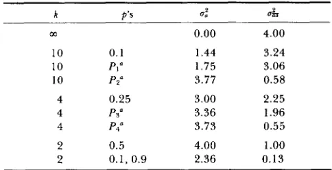
T h e results for a*a effects are simple in comparison to those for dominance effects and involve only 4''s.

T h e a*a variance, a& = 4(1

-

q 2 ) ( 1

-

qi)u:, increases as k and k' increase and decreases as allelic frequency variation for given k and k' increase. T h e coefficient is actually the product of the two coefficients,

2( 1

-

q 2 ) and 2( 1

-

qi), for V , and VL without domi-

nance. Consequently, the coefficient decreases as k and k' increase and increases generally as allelic frequency variation increases. Some values of the coefficients are tabulated in Table 4 for various combinations of k and p's which are the same at both loci.

There are several plausible situations in Table 4

where the a*a variance in is larger than a&. When k is large and the variance of allelic frequencies small, most of the variance is us.

DISCUSSION

Without dominance in the Bmodel the gene effects may be arbitrary. Then, for a specific set of gene frequencies, the additive variance in an infinite population is u: = 2C, p , ( X ,

-

a'.

The assumption of

TABLE 4

Coefficients of u: in u: and uk for various combinations of k

and p's which are the same at both loci

k P ' S d a&

m 0.00 4.00

10 0.1 1.44 3.24

10 PI" 1.75 3.06

10 PZY 3.77 0.58

4 0.25 3.00 2.25

4 Ps" 3.36 1.96

4 P4O 3.73 0.55

2 0.5 4.00 1

.oo

2 0.1, 0.9 2.36 0.13

a P I , Pz, Pa and P q are the same as in Table 2.

random x ' s from some distribution facilitates the treatment of the effects of the number of alleles and of variation in allelic frequencies in terms of u,2 = 2(1

-

q2)& (COCKERHAM and TACHIDA 1987). T h e distribution of X is immaterial except in the sense that

a: may differ among distributions.

T h e introduction of dominance into the 39 model, while cumbersome, involving absolute differences of gene effects, does permit interpretation of the degree of dominance of the favorable allele and extends this interpretation to multiple alleles regardless of any assumptions about the 9 ' s . The assumption of random 9 ' s from some distribution with mean

3

and variance

u&

allows the study of the effects of

3

and

u& on the genetic components in conjunction with

k

and p's. While the formulation will accommodate overdominance,

9 >

1, or underdominance, 3

<

-1, we have confined our attention to dominance within the limits 1 and -1 for complete dominance since there is little or no evidence for dominance outside this range. A possible distribution for 9 is the uniform. This would limit the variance of 9 to u&

(6)

With dominance, the distribution of X becomes important, the main distinction being between skewed and symmetrical distributions. For symmetrical distributions v = 0. We chose the exponential distribution to illustrate the effects of extreme asymmetry. Ac- tually, little is known about the distribution of allelic effects for quantitative characters. Also, we have in- terpreted favorableness of an allele in terms of having a larger X , a feature that can be reversed by a reversal of scale if necessary. A reversal of skewness, however, reverses the sign of v and the contribution of vga,‘ to

if

and dl for the same

3.

We have given equal status to positive and negative values in the treatment of

3.

In practice

9

is probably not negative. There is generally an inbreeding depression in strict outbreeders and little to no inbreeding depression in strict inbreeders for quantitative characters.

All effects and genetic components for the 9 model have been defined for the infinite random mating population. T h e total variance in this population is

ii

+

6::

+

&

summed over loci and ignoring higher order epistatic effects. If our interest were just in this population we could have confined our attention to the effects of the distribution of X’s and 2’s in conjunction with

9,

&

and gene frequencies on these

three components. We have included the other components, d l , d2 and

i,

involving dominance, so that

the results can be extended to include populations or relatives with drift or inbreeding. For example, the additive variance, a;., in finite populations (COCKER-

HAM 1984) for a single locus was shown to be

if.

= (1

-

8 ) ~ :

+

2(8

-

y

-

2 A

+

2 6 ) d

+

4(8

-

y) dl

+

2(y - 6) d2

+

2(7 - A ) i

where 8, 7 , 6, and A are the identity by descent measures for two, three, and four genes and two gene pairs, respectively, dependent on the drift status of the populations. T h e coefficients are all positive. Of interest is the loss in additive variance,

~ 2 .

- ol, with drift. Assuming

9 > 0 and

X either symmetrically distributed or skewed to the right, d l is negative and

contributes to the loss. Also, OCT: represents a loss but the other components represent gains (although often insignificant ones).

T h e inclusion of a*a epistatic effects had much simpler consequences than that of dominance effects.

T h e assumption of random effects again allowed an analysis of u& and the a*a variance in a? in terms of

k

and the allelic frequencies.

In finite populations there is also a contribution of u& to .:a in the sum over loci within finite populations

(GOODNIGHT 1988; COCKERHAM and TACHIDA 1988). This contribution is 4(8

-

L)o& where is the joint descent measure for two genes at each locus on four distinct gametes. In comparing a: and

2.

we have to take additional account of the loss of a*a variance in

ii

according to (1 - 8) and the gain due to

4(8

-

i)&

and of the relative values of

d‘

and d .

Then, we can make quantitative comparisons between the additive variance in finite populations and that in the original population. T h e same procedure can be utilized for comparing the dominance and a*a variance of the two populations.

More important, it is the complete set of genetic components for the P m o d e l that is required to pre- dict the immediate or permanent response to selection for various populations.

BRUCE S. WEIR and MICHAEL TURELLI and two anonymous review,ers provided helpful comments on the presentation of these results. Paper No. 1 1726 of the Journal Series of the North Carolina A,pricultural Research Service, Raleigh, North Carolina 27695- 7643. This investigation was supported in part by National Insti- tutes of Health Grant GM 11546 from the National Institute of

General Medical Sciences.

L I T E R A T U R E CITED

COCKERHAM, C. C., 1984 Covariances of relatives for quantitative characters with drift, pp. 195-208 in Human Population Ce-

netics: The Pittsburgh Symposium, edited by A . CHAKRAVARTI. Van Nostrand Reinhold, New York.

COCKERHAM, <:. C., and D. F. MATLINGER, 1985 Selection response based on selfed progenies. Crop Sci., 25: 483-488. COCKERHAM, C . C., and 1-1. TACHIDA, 1987 Evolution and main-

tenance of quantitative genetic variation by mutations. Proc. Natl. Acad. Sci. USA 84: 6205-6209.

COCKERHAM, C . C., and H. TACHIDA, 1988 Permanency of response to selection for quantitative characters in finite populations. Proc. Nati. Acad. Sci. USA 85: 1563-1565.

COMSTOCK, R. E., and H. F . ROBINSON, 1948 T h e components of genetic variance in populations of biparental progenies and their use in estimati:lg the average degree of dominance. Biometrics 4: 254-266.

COODNIGHT, C. J . , 1988 Epistasis and the effect of founder events on the additive genetic variance. Evolution 42: 441-454. HARRIS, D. L., 1964 Genotypic covariances between inbred rela-

tives. Genetics 50: 13 19-1 348.

TACHIDA, H., and C. C. COCKERHAM, 1987 Quantitative genetic variation in an ecological setting. Theor. Popul. Biol. 32: 393- 429.

WRIGHT, A . J., and C. C . COCKERHAM, 1985 Selection with partial selfing. I. Mass selection. Genetics 109: 585-597.