Abstract
ANANTARAMAN, ARAVINDH VENKATASESHADRI
Reducing Frequency in Real-Time Systems via Speculation and Fall-Back Recovery (Under the direction of Dr. Eric Rotenberg)
In real-time systems, safe operation requires that tasks complete before their deadlines. Static worst-case timing analysis is used to derive an upper bound on the number of cycles for a task, and this is the basis for a safe frequency that ensures timely completion in any scenario. Unfortunately, it is difficult to tightly bound the number of cycles for a complex task executing on a complex pipeline, and so the safe frequency tends to be over-inflated. Power efficiency is sacrificed for safety.
The situation only worsens as advanced microarchitectural techniques are deployed in embedded systems. High-performance microarchitectural techniques such as caching, branch prediction, and pipelining decrease typical execution times. At the same time, it is difficult to tightly bound the worst-case execution time of complex tasks on highly dynamic substrates. As a result, the gap between worst-case execution time and typical execution time is expected to increase.
to a higher recovery frequency that ensures the overall deadline is met in spite of the interim misprediction.
The primary contribution of this thesis is the development of two new frequency speculation algorithms. A drawback of the original frequency speculation algorithm is that a sub-task misprediction is detected only after completing the sub-task. The misprediction can be detected earlier through the use of a watchdog timer that expires at the checkpoint unless the sub-task completes in time to advance it to the next checkpoint. Early detection is superior because recovery can be initiated earlier, in the middle of the mispredicted sub-task. This introduces extra slack that can be used to lower the speculative frequency even further.
Reducing Frequency in Real-Time Systems via Speculation and Fall-Back Recovery
by
Aravindh Venkataseshadri Anantaraman
A thesis submitted to the graduate faculty of
North Carolina State University
In partial fulfillment of the requirements of the degree of
Master of Science
COMPUTER ENGINEERING
Raleigh
2003
Approved by
________________________________
Dr. Eric Rotenberg, Chair of the Advisory Committee
__________________________ _____________________________
Dr. Gregory T. Byrd Dr. Alexander G. Dean
________________________________
BIOGRAPHY
Aravindh Venkataseshadri Anantaraman was born on 29th October 1979 in the
Union Territory of Pondicherry, India. In 2001, he graduated with a B.E (Honors) degree in Electrical and Electronics Engineering from the Birla Institute of Technology and Science (BITS), Pilani, Rajasthan, India. He was an intern with Motorola GSM design center at Bangalore, India between July and December 2000.
Acknowledgements
First, I would like to thank my parents Anantaraman and Rukmani for their support. I cannot describe in words my gratitude for them for all they have done for me.
I would like to thank my graduate advisor, Dr. Eric Rotenberg, for having given me the opportunity to work under him. He is a fantastic teacher and I have learned a lot from him about computer architecture and about research. His enthusiasm and energy have influenced me a lot. He has shown tremendous confidence in me and I am indebted to him. His way of expressing things clearly and without ambiguity continues to amaze me. His writing style is the best that I have seen and I have tried my best to write this thesis to meet his high standards.
Sincere appreciation is due to Dr. Frank Mueller for his guidance and his valuable suggestions during the course of this project. I would also like to specially thank him for permission to use the static timing analyzer tool developed by him.
I also thank Dr. Gregory Byrd, Dr. Alexander Dean, and Dr. Frank Mueller for having agreed to be on my thesis committee and for their valuable comments after reviewing my thesis.
I would like to thank my colleague on this project Kiran Seth. It was a great experience working with him. He was fully responsible for fixing the static timing analyzer tool used in this thesis.
I would also like to thank the other members of my research group - Zach Purser, Karthik Sundaramoorthy, and Jinson Koppanallil - for having helped me out on various occasions. Zach’s critical comments have been very thought-provoking and have helped me to look at this research from different perspectives. Special acknowledgements are due to Steve Lipa and David Winick for their help while at 301 EGRC.
My friend Vishwanath Sundararaman has been a great help. He is a great source of inspiration to me. He has helped me out in crunch times and I am thankful to him for his support.
I am deeply indebted to Lashminarayan Venkatesan and Udayakumar Shanmugam for their help in various ways.
Friends who have helped me in numerous ways include Uma Raghuraman, Prasanna Venkatesh, Balaji Sundar, Anand Natarajan, Karthik Subramanian, Narayanan Chandrasekar, Geethapriya Thamilarasu, Anupama Balasubramanian, Anand Parthasarathy, Visvanathan Hariharan, Mohamed Sheik Nainar, Jaikumaran Cancheevaram, Srivatsan Ravindran, Sajjan Raghavan, Pradeep Mahadevan, Karthikeyan Santhanagopalan, Manukaran Karunakaran, Arianathan Rajagopal, Patrick Hamilton, Yogesh Ramados, Subhashini Sivagnanam, Anita Nagarajan…the list is endless. I thank them all for their support.
I would like to take this opportunity to thank my friends from high school Varadarajan Sridharan, Denis Joe David, and Namassivayam Sandrasse. They have been a constant source of support to me.
TABLE OF CONTENTS
LIST OF FIGURES ... vii
LIST OF TABLES... xi
LIST OF EQUATIONS ... xii
Chapter 1 Introduction ... 1
1.1 Contributions ... 5
1.2 Thesis Organization ... 7
Chapter 2 Related Work... 8
Chapter 3 Frequency Speculation Algorithms... 11
3.1 Frequency Speculation Overview... 12
3.2 Terminology... 17
3.3 Frequency Speculation Algorithms ... 19
3.3.1 No speculation ... 20
3.3.2 Original frequency speculation algorithm... 20
3.3.3 Early-detection logical re-execution algorithm... 24
3.3.4 Early-detection continuous-execution algorithm... 26
Chapter 4 System Requirements and Design... 33
4.1 Hardware Support ... 33
4.1.1 Watchdog counter ... 34
4.1.2 Multiple frequency/voltage settings... 34
4.1.3 Hardware registers ... 35
4.1.3.1 Profiling register ... 35
4.1.3.2 Frequency registers ... 36
4.2 Off-line Software Support ... 36
4.2.1 Static worst-case timing analysis ... 36
4.2.2 Sub-task selection ... 40
4.3 Run-Time Software Support... 41
4.3.1 Run-time system component... 42
4.3.1.1 Setting PETs... 42
4.3.1.2 Recomputing frequencies... 46
4.3.1.3 Pre-computing checkpoint information ... 46
4.3.2 Management of hardware registers ... 48
4.3.2.1 Management of the watchdog counter... 49
4.3.2.2 Management of profiling counter ... 49
4.3.2.3 Management of the frequency registers... 50
Chapter 5 Experimental Framework... 51
5.1 Simulator Description... 51
5.2 Power Modeling... 52
5.3 Benchmarks ... 53
Chapter 6 Results ... 54
6.1.2 Varying PETs through on-line profiling ... 60
6.1.3 Effect of WCET analysis ... 64
6.2 Power Results ... 68
6.3 Effects of Sub-task Selection... 72
Chapter 7 Summary and Future Work... 75
Bibliography ... 79
LIST OF FIGURES
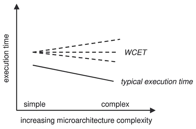
Figure 1-1. Effect of microarchitectural techniques on actual and worst-case execution
times... 4
Figure 3-1. Timing of a task with no mispredictions... 13
Figure 3-2. Timing of a task with one misprediction and late-detection. ... 14
Figure 3-3. Timing of a task with one misprediction and early-detection... 14
Figure 3-4. Advantage of early detection over late detection... 16
Figure 3-5. Timing of a real-time task in a system implementing the original frequency speculation algorithm... 21
Figure 3-6. Timing of a real-time task executed on a system implementing the early-detection logical re-execution algorithm... 24
Figure 3-7. Timing of a real-time task executed on a system implementing the early-detection and continuous-execution algorithm. ... 28
Figure 3-8. Timeline of the mispredicted sub-task in the early-detection continuous-execution scheme. ... 29
Figure 4-1. Overview of the timing tool[6][19][18][17][16][7]. ... 37
Figure 4-2. Run-time software support showing light-weight code snippets and run-time system. ... 42
Figure 4-3. Setting PET on the basis of a target misprediction rate. ... 45
Figure 4-4. Maintenance of watchdog counter by code snippets within a task. ... 49
Figure 6-1. (a) Speculative and (b) recovery frequencies generated by different frequency speculation algorithms for decreasing deadlines for ‘adpcm’.... 57
Figure 6-2. (a) Speculative and (b) recovery frequencies generated by different frequency speculation algorithms for decreasing deadlines for ‘cnt’.... 57
Figure 6-3. (a) Speculative and (b) recovery frequencies generated by different frequency speculation algorithms for decreasing deadlines for ‘fft’.... 57
Figure 6-4. (a) Speculative and (b) recovery frequencies generated by different frequency speculation algorithms for decreasing deadlines for ‘lms’.... 58
Figure 6-6. (a) Speculative and (b) recovery frequencies generated by different frequency speculation algorithms for decreasing deadlines for ‘srt’.... 58 Figure 6-7. Worst-case, speculative, and recovery frequencies generated by the original frequency speculation algorithm for decreasing deadlines for ‘adpcm’.... 59 Figure 6-8. Worst-case, speculative, and recovery frequencies generated by the
early-detection re-execution algorithm for decreasing deadlines for ‘adpcm’.... 59 Figure 6-9. Worst-case, speculative, and recovery frequencies generated by the
Figure 6-20. Power savings for different frequency speculation algorithms for a tight deadline, assuming (a) perfect clock gating and (b) perfect clock gating with standby power... 69 Figure 6-21. Energy savings for different frequency speculation algorithms for a tight deadline, assuming (a) perfect clock gating and (b) perfect clock gating with standby power... 69 Figure 6-22. Savings in power for different frequency speculation algorithms for a loose deadline assuming (a) perfect clock gating and (b) perfect clock gating with standby power... 70 Figure 6-23. Savings in energy for different frequency speculation algorithms for a loose deadline assuming (a) perfect clock gating and (b) perfect clock gating with standby power... 70 Figure 6-24. Power savings for different frequency speculation algorithms for a tight deadline, assuming (a) perfect clock gating and (b) perfect clock gating with standby power, with 20 mispredictions out of 200 task executions... 71 Figure 6-25. Energy savings for different frequency speculation algorithms for a tight deadline, assuming (a) perfect clock gating and (b) perfect clock gating with standby power, with 20 mispredictions out of 200 task executions... 72 Figure 6-26. (a) Speculative and (b) recovery frequencies generated by the original frequency speculation algorithm for various sub-task selection methods, for ‘adpcm ’. ... 74 Figure 6-27. (a) Speculative and (b) recovery frequencies generated by the
early-detection re-execution algorithm for various sub-task selection methods, for ‘adpcm ’. ... 74 Figure 6-28. (a) Speculative and (b) recovery frequencies generated by early-detection continuous-execution algorithm for various sub-task selection methods, for ‘adpcm ’. ... 74
Figure A-1. Worst-case frequency, speculative, and recovery frequencies generated by the original frequency speculation algorithm for varying deadlines, for ‘cnt’.... 81 Figure A-2. Worst-case frequency, speculative, and recovery frequencies generated by the early-detection re-execution algorithm for varying deadlines, for ‘cnt’.... 81 Figure A-3. Worst-case frequency, speculative, and recovery frequencies generated by the early-detection continuous-execution algorithm for decreasing deadlines, for
LIST OF TABLES
Table 4-1. Frequency (MHz)/voltage (V) settings... 35
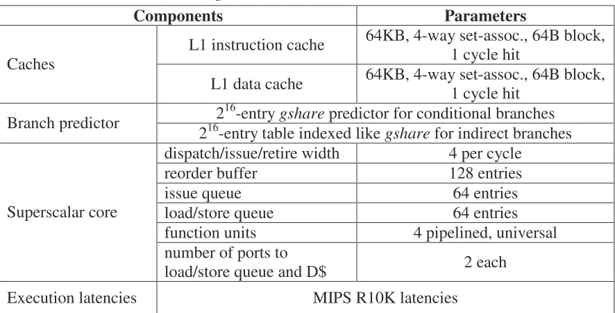
Table 5-1. Microarchitecture configuration... 51
Table 5-2. Frequency (Mhz) /memory latency (cycles) ... 52
LIST OF EQUATIONS
Equation 3-1. Computing the worst-case frequency... 20
Equation 3-2. Mathematical representation of the original frequency speculation model. ... 22
Equation 3-3. Mathematical representation of the early-detection logical re-execution algorithm. ... 25
Equation 3-4. Simplified form of Equation 3-3... 26
Equation 3-5. Mathematical equivalent of the early-detection continuous-execution algorithm. ... 28
Equation 3-6. Number of cycles of the mispredicted sub-task at the recovery frequency. ... 30
Equation 3-7. Number of cycles that remain and must be completed at the recovery frequency... 30
Equation 3-8... 30
Equation 3-9... 30
Equation 3-10... 31
Equation 3-11. Mathematical representation of the early-detection continuous-execution algorithm. ... 31
Equation 3-12. Simplified form of Equation 3-11... 31
Equation 4-1. Checkpoint for sub-task i computed using the forward checkpointing method... 46
Equation 4-2. Checkpoint for sub-task i using the backward checkpointing method, assuming early-detection logical re-execution algorithm. ... 47
Chapter 1 Introduction
In hard real-time systems, it is critical to ensure that a task always finishes before its deadline. Missing a deadline could have potentially hazardous effects. To guarantee safety, designers of real-time systems estimate an upper bound on the number of cycles needed for the task. The upper bound should be safe, i.e., it should always be greater than the actual execution time even in the worst possible scenario.
Static worst-case timing analysis is a means for automatically deriving a safe upper bound for the execution time. Static timing analysis performs a traversal of all possible execution paths of a program and identifies the longest execution path. More importantly, static timing analysis accounts for both program uncertainty (path uncertainty due to input dependencies, statically unknown addresses, etc.) and also microarchitectural uncertainty, (pipelining, caching, dynamic branch prediction, etc.). Unfortunately, due to the complexity of the analysis and the constraint of ensuring a safe bound, the analysis is very conservative and the upper bound on the execution cycles is typically over-inflated.
To ensure safety, the minimum clock frequency needed by the system depends on the worst-case number of cycles for a task and the task deadline.
deadline cycles case
-worst
Ideally, the worst-case number of cycles should be close to the typical number of cycles, so that the frequency is close to the frequency needed in practice. Over-inflation of the worst-case bound leads to a correspondingly over-inflated frequency.
Static frequency speculation, proposed by Rotenberg [22], is a method by which a task is executed at a low speculative frequency, derived using typical execution times. Progress of the speculative task is periodically gauged. If the task is making satisfactory progress, the system continues executing the task at the speculative frequency. Otherwise, it is assumed that continued execution of the task at the speculative frequency could potentially lead to the task missing its deadline. To avoid this, the system falls back to a higher but safe recovery frequency. The recovery frequency is derived using the worst-case execution times (WCET) obtained from worst-worst-case analysis.
Reducing the system frequency by running at a low speculative frequency most of the time has benefits. Probably the most important and direct benefit is savings in power. Power is directly proportional to processor voltage and frequency by the fundamental relation P α fV2. Clocking the processor at a lower frequency means that circuits are permitted to run slower. Lowering supply voltage is a way of slowing down circuits. This technique of reducing frequency and hence voltage is called dynamic voltage scaling (DVS) [21]. Frequency speculation, coupled with DVS, results in cubic reductions in power. In addition, DVS contributes to savings in energy since energy varies directly as the square of voltage (E α V2). Thus, frequency speculation, in conjunction with DVS,
enables significant savings in power and energy.
execution time and actual execution time. Figure 1-1 illustrates this trend qualitatively. Increasing microarchitectural complexity is shown on the X-axis and execution time on the Y-axis. While it is true that typical execution time scales down as microarchitectural complexity increases, the statically-derivable worst-case execution time may decrease at a slower rate, stay roughly the same, or even increase. However, irrespective of the scaling of WCET, reduction in actual execution time (brought about by the above mentioned microarchitectural techniques) will most likely increase the gap between worst-case execution time and typical execution time as shown in the figure. Since frequency speculation efficiently reconciles this gap, it is especially important that frequency speculation be employed in future embedded processors.
WCET
typical execution time
increasing microarchitecture complexity
ex
ec
ut
io
n
tim
e
simple complex
WCET
typical execution time
increasing microarchitecture complexity
ex
ec
ut
io
n
tim
e
simple complex
1.1 Contributions
The contributions of this thesis are as follows.
• Two new static frequency speculation algorithms have been proposed in this thesis that significantly outperform the original static frequency speculation algorithm [22]. The mathematical models for these algorithms have been derived. The key innovation is detecting mispredictions early, by means of a watchdog timer, namely at the checkpoint instead of at sub-task completion. This modification further decouples the speculative frequency from the worst-case execution time.
• Hardware and software requirements for static frequency speculation have been identified and described in detail.
• Sub-task selection is essential for implementing the proposed frequency speculation algorithms. Rotenberg’s initial published work implemented sub-task selection by concatenating sixteen FFT programs to form the hard-real time task, each FFT program representing a sub-task [22]. This thesis takes a step forward and performs actual sub-task selection for six real-time benchmarks, albeit manually.
known initially, the initial predicted execution time is set to be equal to the worst-case execution time. Since the actual execution times may vary over time, the predicted execution times have to be updated periodically to reflect the actual execution times. Rotenberg proposed using off-line simulation to predict the execution times [22]. A key contribution of this thesis is an on-line method for profiling the actual execution times of the sub-tasks, and periodically updating the predicted execution times based on a target misprediction rate.
• A simulation framework, with the necessary hardware and software support for frequency speculation, has been developed during the course of this thesis. This environment accurately models a real-time system employing frequency speculation, including the processor, the run-time system, and sub-task delineated tasks.
1.2 Thesis Organization
Chapter 2 Related Work
This thesis is closely related to the work of Rotenberg [22] and is as an extension of that research. My work shares key aspects with the original work, including (1) exploiting the large gap between actual execution times and WCET, (2) dividing the task into smaller sub-tasks to gauge the progress, and (3) implementing static speculation, in which the speculative and recovery frequencies are computed in advance and remain fixed during the execution of the task. However, some new techniques have been developed that are unique to this thesis. One such technique is early misprediction detection, in which a misprediction is detected as early as the checkpoint via a watchdog timer, unlike the earlier method in which a misprediction is detected only at the end of the sub-task. Sub-task selection has been done manually for six real-time benchmarks and this has helped establish that it is indeed possible to do sub-task selection. In the earlier work, off-line simulations were used to estimate the predicted execution times, whereas this thesis uses an on-line profiling mechanism implemented in the real-time system. The earlier work presented savings in terms of frequency, whereas here, power and energy savings are reported using the Wattch [3] power models adapted for a contemporary superscalar microarchitecture.
speculative and recovery frequencies for a task as a whole and they do not change during the lifetime of the task.
Using our static frequency speculation approach, there are at most two frequency switches during a real-time task. The first frequency switch is at the beginning of the task, when the system sets the processor frequency to the speculative frequency computed for that task. If there is a misprediction, a second switch occurs when the system falls back to the recovery frequency. A dynamic speculation scheme, like the one proposed by Mossé et al [15], may yield greater power savings by tracking small changes in the frequency demands of the task. However, the overhead of continuously monitoring the available slack, recomputing the frequency accordingly, and switching frequencies often, can be significant (especially in systems where the frequency-switching overhead is significant).
Much research has been done in using dynamic voltage/frequency scaling to reduce power consumption in general purpose computers [8][9][14][26]. The general idea is to adjust frequency to reduce power consumption by predicting future processor utilization, while maintaining performance.
Chapter 3 Frequency Speculation Algorithms
Safe planning in real-time systems requires having upper bounds for the execution times of tasks. The worst-case execution time (WCET) is statically derived either manually by the designer or automatically by a timing analyzer integrated with the compiler. Correct worst-case timing analysis ensures that WCET is never underestimated. At the same time, overestimation of WCET is minimized as much as possible. However, as microarchitectural complexity increases, WCET may become increasingly exaggerated due to analysis complexity. Since WCET is used as a basis for computing the lower frequency bound of the real-time system, the frequency needed to guarantee a safe system is also highly inflated.
Static frequency speculation has been shown to significantly reduce frequency while maintaining system safety.
3.1 Frequency Speculation Overview
As previously mentioned, the hard real-time task is divided into smaller portions called sub-tasks. The process of splitting up the task into sub-tasks is called sub-task selection. Sub-task selection can be performed manually by the programmer or automatically by the compiler.
Each sub-task has its own interim deadline, called a checkpoint. A sub-task is expected to complete before its checkpoint at the speculative frequency. Continued safe progress of the task as a whole is confirmed by successfully completing a sub-task before its checkpoint. Note that checkpoints are soft deadlines and their purpose is only to gauge progress at the speculative frequency. Hence, a checkpoint can be missed without compromising overall safety. Recovery ensures that the overall task deadline will still be met in spite of missing a checkpoint.
Missed checkpoints are detected by means of a hardware watchdog timer. The setting of the checkpoints and the operation of the watchdog timer will be described in detail in Chapter 4.
the recovery frequency. How the mispredicted sub-task itself is handled depends on the frequency speculation algorithm, as we explain below. The mispredicted sub-task is special in that it is unfinished when the watchdog timer expires.
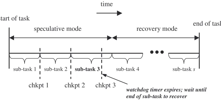
Figure 3-1 shows the timing of a task in which all the sub-tasks are correctly predicted (and hence has no mispredictions). The entire task is run at the speculative frequency since there are no mispredictions. Figure 3-2 and Figure 3-3 show the timing of a task in which one of the sub-tasks is mispredicted. There is a key difference in the method for detecting the misprediction, as illustrated in the two figures. In the late-detection model (Figure 3-2), the value in the watchdog timer is examined on the completion of the sub-task. If the value is zero (expired), it means that the actual execution time of the sub-task is more than its predicted execution time. Thus, a misprediction must have occurred, so remaining sub-tasks are executed at the recovery frequency.
speculative mode time
chkpt 2 chkpt 3 chkpt 4
sub-task 1 sub-task 2 sub-task 3 sub-task 4 sub-task s
start of task end of task
chkpt 1
sub-task 1
speculative mode recovery mode
chkpt 1 chkpt 2 chkpt 3 watchdog timer expires; wait until
end of sub-task to recover
sub-task 2 sub-task 3 sub-task 4 sub-task s
start of task
end of task time
Figure 3-2. Timing of a task with one misprediction and late-detection.
sub-task 3
speculative mode recovery mode
chkpt 1 chkpt 2 chkpt 3 watchdog timer expires; start
recovery immediately
sub-task 1 sub-task 2 sub-task 4 sub-task s
start of task
end of task time
Figure 3-3. Timing of a task with one misprediction and early-detection.
of the mispredicted sub-task at the recovery frequency. In the early detection method (Figure 3-3), the watchdog timer raises an interrupt as soon as it expires (actual execution time exceeds predicted execution time).
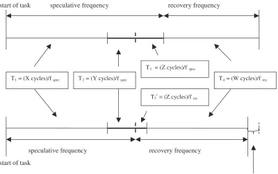
Figure 3-4 shows the advantage of early detection over late detection. Two identical tasks with the same mispredicted sub-task (highlighted) are shown. The first case employs late detection, while the second employs early detection. The correctly predicted sub-tasks (prior to the mispredicted sub-task) and the subsequent sub-tasks (after the mispredicted sub-task) are not explicitly delineated. The amount of work in the correctly predicted sub-tasks (say X cycles) is the same in both cases. For the same frequency fspec,the time spent is equal to X/fspec (shown as T1 in the figure) for both cases.
Similarly, the amount of work for the sub-tasks after the mispredicted sub-task (say W cycles) is the same in both cases and hence the amount of time needed for the remaining sub-tasks is W/frec (shown as T4 in the figure) for both cases, for the same recovery
frequency frec. Consider now the amount of time needed for the mispredicted sub-task.
The amount of work completed before the checkpoint (say Y cycles) is the same since both cases have the same speculative frequency. The time taken is Y/fspec (shown as T2 in
the figure). Let Z be the amount of work (in cycles) remaining after the checkpoint. In the first case, the remaining work (Z cycles) is executed at the speculative frequency (T3 =
Z/fspec), whereas in the second case, the unfinished work is executed at the higher
recovery frequency (T3′ = Z/frec). The portion of the mispredicted sub-task after the
the early detection method than for the late detection method as shown in the figure, assuming the same {fspec, frec} pair. The extra slack in the timeline generated by initiating
recovery earlier can be utilized to lower the speculative frequency, in case of early detection.
T1 = (X cycles)/fspec T2 = (Y cycles)/fspec
T3 = (Z cycles)/fspec
T3′ = (Z cycles)/f rec
T4 = (W cycles)/frec
start of task
start of task speculative frequency recovery frequency
speculative frequency recovery frequency
slack gained by running unfinished portion of mispredicted sub-task at recovery frequency
Figure 3-4. Advantage of early detection over late detection.
pessimistic since it assumes no work is completed by the mispredicted sub-task at the speculative frequency (before the misprediction is detected). Nevertheless, as long as the time spent by the mispredicted sub-task until the checkpoint plus the time needed to logically re-execute the sub-task (at the high recovery frequency assuming worst-case conditions) is less than the time needed to execute the entire sub-task at the low speculative frequency assuming worst-case conditions, the early-detection logical re-execution method will outperform late-detection. As we will show, this is often the case.
However, the penalty of logical re-execution is significant and reduces potential frequency savings due to early-detection. To overcome this, a tighter bound for the unfinished work and hence the time needed to complete the unfinished work at the recovery frequency is derived using a more sophisticated analysis. This tighter method, called early-detection continuous-execution, effectively addresses the problems of both late-detection and early-detection with logical re-execution.
3.2 Terminology
The notation that will be used throughout this thesis (to describe the characteristics of the system that uses frequency speculation) is described in this section.
• The total number of sub-tasks in the hard real-time task is denoted by the letter s.
• Frequency is denoted by the letter f.
• fwc denotes the minimum frequency at which the processor should be run such
• fspec represents the speculative frequency as determined by the frequency
speculation algorithm. Typically fspec is much lower than fwc. A system running at
the speculative frequency (fspec) is expected to meet the deadline, but not
guaranteed to do so. Therefore, progress must be continuously gauged and a recovery mechanism deployed as needed.
• frec represents the recovery frequency as determined by the frequency speculation
algorithm. The recovery frequency is the minimum frequency at which the remainder of the task must be executed to ensure that the overall deadline is met in case a sub-task is mispredicted.
• i, j, and k denote individual sub-tasks that constitute the overall task.
• Static worst-case timing analysis is performed by a static timing analyzer on a per sub-task basis. The worst-case execution time of a sub-task is denoted by WCETi,f, where the subscript i denotes the sub-task and the subscript f denotes the
frequency at which WCET is estimated.
• The predicted execution time of a sub-task i at frequency f is denoted by PETi,f.
• The actual execution times of a sub-task i at frequency f is denoted by AETi,f.
Actual execution time is not known until run-time and is not used directly in the analysis that generates the speculative and recovery frequencies.
WCETi,f and PETi,f are the two key inputs for the frequency speculation algorithms
3.3 Frequency Speculation Algorithms
In this section, we describe the various static frequency speculation algorithms used to derive the speculative and recovery frequencies. The speculative and recovery frequencies are derived before the task executes and kept the same for the duration of the task. In this sense, frequency speculation is “static”. However, a run-time software component periodically re-applies the frequency speculation algorithm to update the speculative and recovery frequencies, based on more recent history of actual execution times. (This approach is described in detail in Section 4.3.)
Before describing the frequency speculation algorithms, we define the input parameters needed for the analysis:
• Task deadline.
• Number of sub-tasks.
• Frequency range supported by the microprocessor.
• PETi,f: Predicted execution times for each of the sub-tasks at all supported
frequencies.
• WCETi,f: Worst case execution times for each of the sub-tasks at all supported
frequencies.
overhead depends upon the number of steps between the starting and ending frequencies.
3.3.1 No speculation
The worst-case frequency fwc is derived without speculation, i.e., using only
worst-case execution times.
=
≤
s
1 i
f
i,
deadline
WCET
wcEquation 3-1. Computing the worst-case frequency.
The worst-case frequency fwc for a task, given a deadline, is computed using
Equation 3-1. WCETi,f for all the sub-tasks are substituted into Equation 3-1 starting from
the lowest available frequency and progressively increasing the frequency until the inequality is satisfied. Starting at the lowest frequency and proceeding upwards ensures that we arrive at the minimum value for fwc. It is to be noted that the worst-case frequency
fwc is not needed for frequency speculation purposes. However, it is calculated to provide
a basis for comparison.
3.3.2 Original frequency speculation algorithm
continues to execute the next sub-task at the speculative frequency. However, if a checkpoint is missed (actual execution time exceeds predicted execution time), then that sub-task is said to be mispredicted. On a misprediction, recovery is initiated. All subsequent sub-tasks are executed at the recovery frequency. Note that misprediction detection is late, i.e., a misprediction is detected on completion of the sub-task.
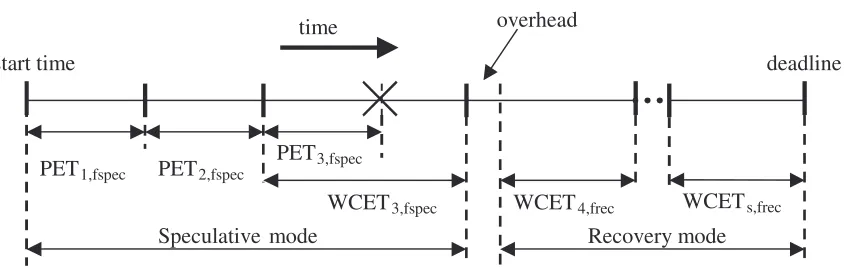
Figure 3-5 shows the timing of a task, complete with sub-tasks and checkpoints. Each speculative sub-task is expected to complete before its checkpoint, meaning its actual execution time should not exceed PETi,fspec. At the end of each speculative
task, the system checks if the task completed before its checkpoint. The third sub-task, marked with a cross, represents a misspredicted sub-task in Figure 3-5. The misprediction is detected at the end of the third sub-task. After a fixed switching overhead, the system falls back to the recovery mode and all the sub-tasks that follow the mispredicted sub-task are run in recovery mode.
time start time
PET1,fspec PET2,fspec
WCET3,fspec WCET4,frec WCETs,frec
Speculative mode Recovery mode
deadline
PET3,fspec
overhead
At the end of the task, the system returns to some other speculative frequency to begin execution of the next task. There is a second switching overhead incurred in this transition from the recovery to the speculative frequency. If the task had no mispredictions, then the frequency is changed from the current speculative frequency to the speculative frequency for the next task.
Equation 3-2 is the mathematical implementation of the original static frequency speculation algorithm. The first term on the left-hand side represents an upper bound on the cumulative execution time of all the correctly predicted sub-tasks, the sum of their PETs at the speculative frequency. The second term is an upper bound on the time taken by the mispredicted sub-task, which is assumed to be the worst-case execution time of that sub-task at the speculative frequency. It is to be noted that the actual execution time of a sub-task, AETi,fspec, is unknown until run-time. If the sub-task completes before its
checkpoint, it means that AETi,fspec is less than or equal to PETi,fspec. However, in the case
of a misprediction, AETi,fspec is greater than PETi,fspec but less than WCETi,fspec. In the
worst case, AETi,fspec would be equal to WCETi,fspec. Hence, for the purpose of safe
analysis, we use WCET at the speculative frequency for the execution time of a mispredicted sub-task.
deadline
WCET
overhead
WCET
PET
1 i1 j
s
1 i k
f k, f
i, f
j, spec
+
spec+
+
rec≤
−
= =+
The third term in Equation 3-2 is the fixed overhead that is incurred when switching from the speculative to the recovery frequency.
To ensure a safe system, the worst-case scenario is assumed for all the remaining sub-tasks that are executed at the recovery frequency. Note that while WCET is assumed for both the mispredicted sub-task (WCETi,fspec) and subsequent sub-tasks (WCETi,frec),
the mispredicted sub-task is executed at the speculative frequency whereas the subsequent sub-tasks are executed at the recovery frequency. The last term in Equation 3-2 accounts for the cumulative execution time of the remaining sub-tasks assuming WCET at the recovery frequency.
The sum of the four terms on the left-hand side of Equation 3-2 must be less than or equal to the deadline specified for the real-time task to ensure a safe system.
Since any one of the s sub-tasks could be the mispredicted sub-task, Equation 3-2 actually represents s inequalities. It is essential that Equation 3-2 be satisfied for all the s sub-tasks to ensure that the deadline will be safely met. The lowest supported frequency is chosen as the starting value for the speculative frequency, and the lowest frec that
satisfies the inequality in Equation 3-2 assuming the first sub-task is mispredicted is determined. It is then checked if this {fspec, frec} pair satisfies the inequality assuming the
second sub-task was mispredicted, and so on for all the s sub-tasks. If there is a sub-task for which there is no frec to satisfy the inequality, the fspec is incremented to the next
an frec for one of them (for that fspec). This process continues until a minimum {fspec, frec}
pair is found that satisfies all s inequalities.
3.3.3 Early-detection logical re-execution algorithm
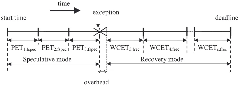
As mentioned in Section 3.1, the late-detection method is not very efficient. The early-detection method was introduced to overcome the deficiencies of the late-detection method. This section describes the early-detection logical re-execution algorithm, which uses the WCET of the entire mispredicted sub-task to conservatively bound the work remaining in a sub-task after a misprediction is detected.
Figure 3-6 illustrates the timing of a task employing the logical re-execution algorithm. The first two sub-tasks are correctly predicted. The third sub-task, denoted by a cross, is mispredicted and the misprediction is detected at its checkpoint. The figure shows the entire mispredicted sub-task to be re-executed (logically). All the remaining sub-tasks are executed at the recovery frequency assuming worst-case execution times.
Speculative mode Recovery mode
start time deadline
PET1,fspec PET2,fspec PET3,fspec WCET3,frec WCET4,frec WCETs,frec
exception time
overhead
Equation 3-3 is the mathematical model for the logical re-execution algorithm. The first term of the inequality represents the cumulative execution time of all the correctly predicted sub-tasks. The second term represents the predicted execution time of the mispredicted sub-task at the speculative frequency. This is the amount of time that elapses before the watchdog timer raises an exception. The third term represents the overhead incurred in switching from the speculative to the recovery frequency. The fourth term very conservatively bounds the remaining time needed by the unfinished, mispredicted sub-task, at the recovery frequency. The simplest way to bound the remaining time is to use the WCET of the entire sub-task; hence it seems like the sub-task is “re-executed” (in fact, it continues normally, i.e., re-execution is apparent only in the mathematical expression). The fifth expression is the sum of the worst-case execution times of the sub-tasks after the mispredicted sub-task while running at the recovery frequency. The sum of these five terms should be less than or equal to the deadline to ensure safe operation.
deadline
WCET
WCET
overhead
PET
PET
1 i
1 j
s
1 i k
f k, f
i, f
i, f
j, spec
+
spec+
+
rec+
rec≤
−
= =+
Equation 3-3. Mathematical representation of the early-detection logical re-execution algorithm.
The mispredicted sub-task is assumed to be logically re-executed at the recovery frequency only for the purposes of analysis. In reality, the mispredicted sub-task is not re-executed from the beginning of the sub-task. Only the unfinished portion of the mispredicted sub-task is actually executed at the recovery frequency. For the purpose of analysis, it is safe to assume that the worst-case execution time of the entire sub-task at the recovery frequency (WCETi,frec) is a safe upper bound for the execution time of any
part of that sub-task assuming worst-case conditions. This algorithm is pessimistic in the sense that it assumes no useful work was done by the mispredicted sub-task at the speculative frequency.
Equation 3-3 can be simplified by merging the PET and WCET terms of the mispredicted sub-task with the corresponding summation terms as shown in Equation 3-4.
deadline
WCET
overhead
PET
i
j
s
i k
f k, f
j, spec
+
+
rec≤
=1 =
Equation 3-4. Simplified form of Equation 3-3.
3.3.4 Early-detection continuous-execution algorithm
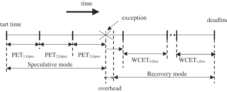
of the mispredicted sub-task, thereby introducing more slack in the schedule and reducing the speculative frequency further.
In this algorithm, an exception is raised when a misprediction is detected and the unfinished portion of the mispredicted sub-task is executed at the recovery frequency. The early-detection continuous-execution algorithm estimates the amount of work that has been completed at the speculative frequency, and from this computes a tight bound for the amount of time needed to complete the unfinished portion of the mispredicted sub-task at the recovery frequency. The remaining sub-tasks are executed at the recovery frequency as in the previous algorithms.
Speculative mode
Recovery mode PET1,fspec PET2,fspec PET3,fspec
WCET4,frec WCETs,frec
start time deadline
time
overhead
exception
Figure 3-7. Timing of a real-time task executed on a system implementing the early-detection and continuous-execution algorithm.
Equation 3-5 is the overall equation that implements the early-detection and continuous-execution algorithm. The first term is the sum of the predicted execution times of the correctly predicted sub-tasks at the speculative frequency. The second term is the amount of time spent by the mispredicted sub-task at the speculative frequency before the exception is triggered. The third term denotes the amount of time that is needed to complete the unfinished portion of the mispredicted sub-task at the recovery frequency. The fourth term denotes the overhead incurred in switching from the speculative to the recovery frequency. The fifth term denotes the sum of the worst-case execution times of the sub-tasks following the mispredicted sub-task, executed at the recovery frequency.
deadline
WCET
overhead
task
sub
ed
mispredict
complete
to
left
time
PET
PET
s 1 i k f k, 1 i 1 j f i, f j, rec spec spec≤
+
+
−
+
+
+ = − =A
BSpeculative mode Recovery mode
start time PETi,fspec deadline
cycles A,WC,fspec < cycles A,WC,frec cycles B,WC,frec
cyclesi,WC,frec
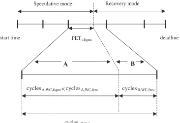
Figure 3-8. Timeline of the mispredicted sub-task in the early-detection continuous-execution scheme.
Figure 3-8 highlights the timeline of the mispredicted sub-task i. Because it was mispredicted, we must assume the worst-case scenario (WC) occurred. Hence, we bound the number of cycles for the entire sub-task using cyclesi,WC,f. Note that the number of
cycles depends on frequency only due to memory effects: the number of cycles to access main memory increases with frequency. The mispredicted sub-task i is partially executed at fspec and partially executed at frec. Since memory cycles increases with frequency, we
We divide the sub-task into two smaller components, A and B. A is the component completed before the misprediction and B is the component left to be done. The upper bound on the number of cycles derived above can be broken down as follows.
cyclesi,WC,frec = cyclesA,WC,frec + cyclesB,WC,frec
Equation 3-6. Number of cycles of the mispredicted sub-task at the recovery frequency.
Since we are interested in bounding the time for B, the unfinished portion, Equation 3-6 is re-arranged as follows.
cyclesB,WC,frec = cyclesi,WC,frec – cyclesA,WC,frec
Equation 3-7. Number of cycles that remain and must be completed at the recovery frequency.
Of course, A is executed at the speculative frequency, not the recovery frequency. We know that cyclesA,WC,fspec < cyclesA,WC,frec because memory cycles increase with
higher frequency. Since the term for A in Equation 3-7 is subtracted from the total number of cycles, it is safe to use a smaller term for A – doing so only increases the number of cycles assumed for B, the unfinished portion. So, Equation 3-7 can be safely re-expressed as follows.
cyclesB,WC,frec ≤ cyclesi,WC,frec – cyclesA,WC,fspec
Equation 3-8.
Now, the number of cycles spent on A is simply the product of the frequency at which A was executed, fspec, and the time spent executing A. The time spent executing A
is the predicted execution time of sub-task i, PETi,fspec. So we get the following
expression.
cyclesA,WC,fspec = PETi,fspec * fspec
Substituting Equation 3-9 into Equation 3-8, we get the following expression. cyclesB,WC,frec≤ cyclesi,WC,frec– PETi,fspec * fspec
Equation 3-10.
The B term can be converted from cycles to time (which is what we want – a bound on the remaining time) by dividing it by the recovery frequency. The right-hand side of Equation 3-10 is also scaled by the reciprocal of the recovery frequency to preserve the inequality.
(cyclesB,WC,frec/frec) ≤ (cyclesi,WC,frec/frec) – (PETi,fspec * fspec /frec)
Equation 3-10 can be re-expressed as follows.
Time left = cylesB,WC,frec/frec = WCETi,frec– (fspec/frec) PETi,fspec
Substituting the above expression into Equation 3-5, we get the final expression for the early detection and continuous execution algorithm as:
deadline WCET overhead PET f f WCET PET PET 1 i 1 j s 1 i k f k, f i, rec spec f i, f i, f
j,spec spec rec spec rec
≤ + + − + + − = =+
Equation 3-11. Mathematical representation of the early-detection continuous-execution algorithm.
By merging the PET term of the mispredicted sub-task into the corresponding summation term, Equation 3-11 can be re-expressed as:
deadline
WCET
PET
f
f
WCET
overhead
PET
i 1 j s 1 i k f k, f i, rec spec f i, fj, spec rec spec rec
≤
+
−
+
+
= =+Similar to the previous algorithms, Equation 3-12 has to be satisfied for all s sub-tasks, since any one of the s sub-tasks could be the mispredicted sub-task. The minimum {fspec, frec} pair that satisfies the above inequality for all s sub-tasks is determined
Chapter 4 System Requirements and Design
To implement frequency speculation in a real-time system, both software and hardware support are needed. Hardware support includes a watchdog counter, a cycle counter for measuring actual execution times of sub-tasks, and two registers that control the speculative and recovery frequency settings. Software support consists of off-line and run-time components. Off-line software support includes static worst-case timing analysis and sub-task selection. Run-time software support consists of management of hardware registers/counters at sub-task boundaries, and periodically re-calculating frequencies and checkpoints, according to the frequency speculation algorithm.
This chapter describes in detail both the hardware and software requirements and their implementation. Section 4.1 describes the hardware support. The off-line and run-time software support are discussed in Section 4.2 and Section 4.3, respectively.
4.1 Hardware Support
4.1.1 Watchdog counter
The processor provides a watchdog counter. It is memory-mapped and hence accessible by software. An initial value can be stored into the watchdog counter via a store instruction. The watchdog counter contents can be read via a load instruction.
The processor decrements the watchdog counter by one every cycle. If it reaches zero, an exception is raised unless watchdog exceptions are disabled by the run-time software.
The watchdog counter is managed by software to detect missed checkpoints. Derivation of watchdog increment values is explained in Section 4.3.1.3.3 while management of the watchdog counter is described in Section 4.3.2.1.
4.1.2 Multiple frequency/voltage settings
A real-time system employing frequency speculation should be equipped with multiple frequency/voltage settings. Processors such as the Transmeta Crusoe, Intel® PXA25x series, and Intel® PXA26x series are good examples of processors with multiple voltage settings [28].
Table 4-1. Frequency (MHz)/voltage (V) settings.
100/0.7 200/0.82 300/0.95 400/1.07 500/1.19 600/1.31 700/1.43 800/1.56 900/1.68 1000/1.8
125/0.73 225/0.85 325/0.98 425/1.1 525/1.22 625/1.34 725/1.46 825/1.59 925/1.71
150/0.76 250/0.89 350/1.01 450/1.13 550/1.25 650/1.37 750/1.5 850/1.62 950/1.74
175/0.79 275/0.92 375/1.04 475/1.16 575/1.28 675/1.41 775/1.53 875/1.65 975/1.77
4.1.3 Hardware registers
This section describes additional hardware resources such as memory-mapped registers, apart from the watchdog counter, that are required to implement the frequency speculation algorithms. Specifically, the processor has to provide three extra memory-mapped registers. One of these three registers is referred to as the profiling register and the other two registers are called frequency registers.
4.1.3.1 Profiling register
The profiling register provides a means to measure the actual execution time of a task. Accumulated profile information is later used in selecting the PET of a sub-task.
4.1.3.2 Frequency registers
The frequency registers are memory-mapped registers. Unlike the watchdog counter and the profiling register, these registers are not incremented or decremented by the hardware. These just contain the current and recovery frequency settings for the current task.
A store to the current frequency register causes the processor to switch to the specified frequency setting. It is assumed that the frequency/voltage combinations are preset in the processor and hence knowledge about the frequency is sufficient to determine the corresponding voltage setting.
A watchdog exception indicates a sub-task was mispredicted. In this case, the processor automatically copies the contents of the recovery frequency register into the current frequency register and therefore switches to that frequency. Note that watchdog exceptions are only enabled for the early-detection schemes. For the late-detection scheme, software must explicitly set the processor frequency to the recovery frequency using the current frequency register.
4.2 Off-line Software Support
4.2.1 Static worst-case timing analysis
properties of the task and can potentially be affected by the input data set. The second is variability due to hardware complexity, such as the pipeline, caches, and branch predictors.
Timing analysis can be performed either dynamically or statically. Dynamic timing analysis is based on simulation. This involves identifying the input data set that causes the longest path to be traversed. A brute force method of trying all possible input combinations to determine the worst-case input may not be practical. Moreover, there is no guarantee that this worst-case input would also induce worst-case behavior in terms of pipeline effects. That is, the program could exhibit worse timing behavior with a different
set of inputs,because of interactions with hardware.
On the other hand, static timing analysis is guaranteed to derive a safe upper bound for the execution time of a task, also called worst-case execution time (WCET).
Figure 4-1. Overview of the timing tool[6][19][18][17][16][7].
program values or variables. The worst-case behavior of architectural components along all execution paths is determined and a bound for the worst-case execution time in cycles is computed [2][6][7][16][17][18][20][24][25].
Figure 4-1 shows the organization of the timing tool used to statically bound WCET for an application. The complete working of the timing tool is beyond the scope of this thesis. A brief synopsis of its various components follows.
The application is compiled using the PISA gcc compiler [4]. Control flow information and references to memory are extracted from the assembly code. It is impossible to bound WCET for unbounded loops. Hence it is essential to provide the upper bound for the number of iterations for each loop.
Using the concept of abstract cache state [2][16], a static cache simulator generates one of four cache categorizations for each memory reference (always miss, always hit, first miss, first hit) to be used by the timing analyzer. The data cache however is not complete at this time. Hence, additional cycles have been padded onto WCET to account for actual data cache misses, obtained via simulation.
resulting WCET may be too pessimistic, although with no tools currently capable of analyzing complex pipelines, this aspect cannot be assessed. To study the effect of tighter WCET, we also decrease WCET without underestimating actual execution times in practice.
The simplified pipeline model is a six-stage, scalar, in-order pipeline. Fetch, decode, register read, execute, memory access, and write-back form the pipeline stages. Only one instruction is fetched per cycle by the fetch unit. Static branch prediction is used. Forward branches are predicted not-taken, while backward branches are predicted taken. The instruction cache and the branch target buffer are merged to simplify analysis, that is, decoded branch targets are stored with the branches in the instruction cache. Instruction fetch is stalled in the case of an indirect branch, i.e., indirect branches are not predicted.
The next component of the timing tool is the timing analyzer. Using the supplied control flow information and loop bounds, cache categorizations from the static cache simulator, and the pipeline specification above, the timing analyzer bounds the timing for each path, then loops, and then functions. Thus the timing analyzer starts with the innermost loops and proceeds outwards until it reaches the outermost level. This hierarchical approach is particularly useful to us since it provides a straightforward means to query WCET for regions of the program. Thus, WCET for a specific sub-task can be easily obtained.
The tool has been used as is from its developers [6][19][18][17][16][7]. No work has been done on the tool as part of this thesis.
4.2.2 Sub-task selection
Sub-task selection is the process of dividing a real-time task into smaller parts. Sub-task selection can be done manually by the programmer or automatically by the compiler (or the static timing analyzer).
Sub-task selection has been done manually for six real-time benchmarks. Certain rules of thumb have been followed while manually selecting sub-tasks.
1. A sufficient number of sub-tasks are selected from the real-time task. 2. Sub-tasks are balanced in terms of execution cycles.
4. A key requirement is that the sub-tasks execute in a linear sequence (complex sub-task graphs are not permitted). The frequency speculation algorithms assume sub-tasks are concatenated to form the task.
Most real-time benchmarks used in this thesis are simple in structure and lend themselves easily to sub-task selection. In particular, sub-task selection has been done by peeling off chunks of iterations from the outermost loop.
4.3 Run-Time Software Support
This section describes run-time software support for frequency speculation. Run-time support can be further divided into two components. The first component is part of the run-time system (for example, the operating system) and hence separate from the task itself. This component periodically selects new PETs on the basis of latest profile information (actual execution times of sub-tasks), re-applies the frequency speculation algorithm to compute new speculative and recovery frequencies, and pre-computes new checkpoint information.
The second component is light-weight, as it is part of the real-time task itself. This component consists of code snippets inserted at sub-task boundaries. The snippets manage the various hardware registers (watchdog counter, profiling register, and frequency registers).
manage the hardware registers. After n executions of task A, the run-time system component selects new PETs and re-computes the speculative and recovery frequencies and the checkpoints. Note that the run-time system component is not a part of task A and is executed between executions of A.
Figure 4-2. Run-time software support showing light-weight code snippets and run-time system.
4.3.1 Run-time system component
This section describes in detail the run-time system components, which includes setting new PETs, re-computing frequencies, and pre-computing the checkpoint information.
4.3.1.1 Setting PETs
Frequency speculation algorithms take advantage of the gap between WCET and PET. Experiments show that the reduction in frequency is directly correlated to the disparity between WCET and PET. A tight estimate for the predicted executed time increases the gap between PET and WCET, thereby increasing the frequency savings. task A (1) task A (2) task A (n) task A (n+1)
time
Light-weight code snippets at sub-task boundaries manage hardware registers, e.g., record actual execution times, set watchdog
A key point is that PETs, as the name suggests, are just predictions of the execution times. The frequency speculation technique ensures safe operation even if the predicted execution times are exceeded during actual execution of the program. Hence, predicted execution times do not need to be safe bounds for execution times, and can be optimistic.
PETs that are too high, that is, which are close to WCET itself, are bad because they lead to high speculative and recovery frequencies. However, if the PETs are too low, the likelihood of mispredicting increases, reducing the power-savings potential of frequency speculation.
Predictions of sub-task execution times are made on the basis of prior actual execution times of the sub-tasks on the target processor. In prior work [22], off-line simulation was used to collect execution times of the sub-tasks and these were used as a basis for PETs. However, off-line simulation is inflexible.
new speculative and recovery frequencies. With new frequencies, the checkpoints and the watchdog increments are re-calculated also.
4.3.1.1.1 Histogram-based prediction method
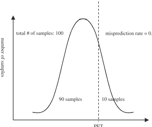
In this method, the history referred to earlier is a histogram of actual execution times. Each time a sub-task executes, the actual execution time is added to its histogram. Periodically, the run-time system examines the histograms and updates the PETs for all sub-tasks based on a pre-defined target misprediction rate. The misprediction rate essentially represents the rate of sub-task mispredictions that can be tolerated by the system. A misprediction rate of zero means that the system has zero tolerance towards mispredictions and the PET is set at the highest non-zero bin. A higher misprediction rate would mean that the PETs can be more optimistic and it is possible that a sub-task might be mispredicted because the PETs might be lower than future actual execution times.
actual execution times of a sub-task (bins)
nu
m
be
r o
f s
am
ple
s
90 samples 10 samples
total # of samples: 100 misprediction rate = 0.1
PET
Figure 4-3. Setting PET on the basis of a target misprediction rate.
An interesting point to consider while setting the misprediction rate is the usage of different misprediction rates for different sub-tasks, since separate histograms are maintained for each sub-task. For example, if the first sub-task is mispredicted, then almost the entire task has to be executed at the recovery frequency. So, a low misprediction rate could be used for earlier sub-tasks. However, the last sub-task mispredicting might not be expensive in terms of power consumption. Also, later sub-tasks can typically utilize slack generated by previous sub-sub-tasks and the chances of mispredicting are fairly low. In such cases, a higher misprediction rate could be used for those sub-tasks.
4.3.1.1.2 Last-N-based prediction method
4.3.1.2 Recomputing frequencies
After setting new PETs for the sub-tasks of a task, the run-time system component applies the frequency speculation algorithm described in Section 3.3, and thereby re-computes the speculative and recovery frequencies for the next N executions of the task.
4.3.1.3 Pre-computing checkpoint information
Checkpoints provide a mechanism to monitor progress of speculative sub-tasks and are critical for safe system operation. Checkpoints are pre-computed by the run-time system component. There are two methods of setting checkpoints: forward checkpointing and backward checkpointing.
4.3.1.3.1 Forward checkpointing
In the forward checkpointing methodology, the checkpoint for a sub-task is the accumulated predicted execution time of the sub-task and all prior sub-tasks at the speculative frequency, as shown in Equation 4-1.
=
=
i1
j j,fspec
i
PET
checkpoint
Equation 4-1. Checkpoint for sub-task i computed using the forward checkpointing method.
4.3.1.3.2 Backward checkpointing
of the mispredicted sub-task, and (3) execute all subsequent sub-tasks at the recovery frequency. As derived in Section 3.3.3, the time needed to complete the unfinished portion of the mispredicted sub-task can be conservatively bounded by the worst-case execution time of the entire sub-task. The time taken to execute the remaining sub-tasks is bounded by the cumulative worst-case execution times of those sub-tasks. The time taken to switch frequency is a fixed overhead. Hence, the checkpoint for sub-task iis as follows.
=
=
s
i
k k,frec
i
deadline
-
overhead
-
WCET
checkpoint
Equation 4-2. Checkpoint for sub-task i using the backward checkpointing method, assuming early-detection logical re-execution algorithm.
Equation 4-2 shows the checkpoint for sub-task i relative to the beginning of the task. Assuming that the total number of sub-tasks is s, the difference between the checkpoint and the deadline is enough to accommodate the frequency switching overhead and the time to execute the entire mispredicted sub-task i and all subsequent sub-tasks at the recovery frequency assuming worst-case conditions.
+
−
−
=
= rec i,fspec
spec s
i
k k,frec
i
PET
f
f
WCET
overhead
deadline
checkpoint
Equation 4-3. Checkpoint for sub-task i using the backward checkpointing method, assuming early-detection continuous-execution algorithm.
4.3.1.3.3 Watchdog increment amounts
The checkpoints are transformed into watchdog increment amounts, for simple management of the watchdog counter. The first sub-task initializes the watchdog counter to the number of cycles between the start of the task and the first checkpoint, which is equal to (checkpoint1*fspec). Each new sub-task adds to the watchdog counter the number
of cycles between the previous checkpoint and its checkpoint. That is, a sub-task i adds ((checkpointi – checkpointi-1) * fspec) cycles to the watchdog counter. As long as sub-tasks
finish before their checkpoints, the watchdog counter will not reach zero (mispredict) before it is incremented by the next sub-task.
Note that by augmenting the watchdog counter instead of overwriting it, extra cycles may accumulate due to sub-tasks that complete ahead of schedule. This slack provides extra time for later sub-tasks. Accumulated slack can lead to the situation where a sub-task exceeds its PET, yet completes before its checkpoint.
4.3.2 Management of hardware registers
4.3.2.1 Management of the watchdog counter
A code snippet at the beginning of the first sub-task initializes the watchdog counter, to the number of cycles between the start of the task and the first checkpoint. A code snippet at the beginning of every subsequent sub-task increments the watchdog counter, using the watchdog increment amounts pre-computed by the run-time system component.
Code snippet initializes watchdog counter at the beginning of the first sub-task
Code snippet augments watchdog counter at the beginning of every sub-task
start time deadline
time
Figure 4-4. Maintenance of watchdog counter by code snippets within a task.
4.3.2.2 Management of profiling counter
![Figure 4-1. Overview of the timing tool[6][19][18][17][16][7].](https://thumb-us.123doks.com/thumbv2/123dok_us/1670800.1210199/51.612.93.500.485.606/figure-overview-of-the-timing-tool.webp)