Disequilibrium Pattern Analysis. I. Theory

(1)

Disequilibrium Pattern Analysis.

I. Theory

Glenys Thomson and William Klitz

Department of Genetics, University of Calijornia, Berkeley, C a l i j k z i a 94720 Manuscript received September 3, 1986

Revised copy accepted May 2, 1987

ABSTRACT

We have developed a method, disequilibrium pattern analysis, for examining the disequilibrium distribution of the entire array of two locus multiallelic haplotypes in a population. It is shown that a

selected haplotype will produce a distinct pattern of linkage disequilibrium values for all generations

while the selection is acting. This pattern will also presumably be maintained for many generations

after the selection event, until the disequilibrium pattern is eventually broken down by genetic drift and recombination. Related haplotypes, sharing an allele with a selected haplotype, assume a value of linkage disequilibrium proportional to the frequency of the unshared allele and have a single negative value of the normalized linkage disequilibrium. The analysis assumes zero linkage disequilibrium for all allelic combinations initially. T h e same basic results continue to apply if the selection involves a new mutant, the occurrence of which creates linkage disequilibrium for some haplotypes. The disequilibrium pattern predicted under selection is robust with respect to the influence of migration and random genetic drift. This method is applicable to population data having linked polymorphic

loci including that determined from protein or DNA sequencing.

HE linkage disequilibrium of haplotypes (chro-

T

mosome or gametic types) formed from tightly linked loci may indicate the nature of past evolutionary events, particularly selection events, acting on the genome. Unlike genotypic ratios, which assume Hardy-Weinberg proportions in one generation in random mating populations, disequilibrium present in haplotypes is retained over generations and its decay over time is a function of recombination between loci. Tightly linked polymorphic loci will retain evidence of distorted haplotypic frequencies for many generations. Thus, the patterns and extent of linkage disequilibrium potentially provide more information for differentiating selection from other evolutionary events than does examination of single locus genetic variation.

In this paper we describe a method, disequilibrium pattern analysis, for examining the disequilibrium distribution of the entire array of haplotypes in a polymorphic two locus system. This method identifies the constraints on the disequilibrium values that a haplotype can assume, and the distribution of the entire array of haplotypes in the disequilibrium space. It is shown that selection leads to specific quantifiable disequilibrium patterns that are robust with respect to the influence of migration and random genetic drift.

Our impetus for developing this methodology was to study the population genetics and evolutionary history of the major histocompatibility complex in humans (HLA). T h e HLA system contains a number

Genetics 1 1 6 623-632 (August, 1987)

of closely linked and highly polymorphic loci, which have strong linkage disequilibrium. There exists an extensive amount of data on the genetic variation for HLA genes in different populations (for example, see the Histocompatibility Testing volumes for 1972, 1980 and 1984, DAUSSET and COLOMBANI 1973; TERASAKI

1980 and ALBERT, BAUR and MAYR 1984).

In this paper we discuss the theoretical aspects of disequilibrium pattern analysis for detecting evolutionary forces acting on a population. T h e companion paper (KLITZ and THOMSON 1987) applies disequilibrium pattern analysis to HLA A and B locus data from a large Danish study (HANSEN et a l . 1979).

RESULTS

Defining the disequilibrium space: T h e linkage disequilibrium parameter

D,

is defined as

where xg is the observed frequency of the haplotype A&

PA,

is the frequency of the allele A, and 98, that of B,, so that the linkage disequilibrium is the difference between the observed haplotype frequency xtl and pA,qBJ, the haplotype frequency expected if the alleles are associated at random. T h e disequilibrium values of the haplotypes of a population are constrained by the relationships

(2)

G. Thomson W. Klitz

where r is the number of alleles at the A locus, and s

the number of alleles at the B locus.

This constraint is most simply illustrated in the case of a two locus, two allele (AI, A2 and B1, B2) model, where the four haplotype frequencies can be ex- pressed as

f(A1B1) = P A 1 q B I

+

D , f ( A d 2 ) = P A 2 q B ,

+

D _{( 3 4}

&Ai&) = P A l q B 2

-

D , _(3b)

Note that P A l

+

P A p = 1 etc., and D is the measure of

linkage disequilibrium (= f(AlBlNA2Bz)

-

f(A182)- f(A2BI)). If the alleles A I and B1 occur together in the haplotype A I B l more often than expected under random association, that is, D

>

0, then the haplotype

A2B2 is also in the positive disequilibrium space. Al-

though the frequency of the haplotype A2B2 will be different from that of the haplotype A I B I , unless

PA^

= q B 1 = 0.5, the constraints given in

(2),

and illustrated in (3a), imply that these two haplotypes will have an equal value of linkage disequilibrium. T h e positive disequilibria are balanced in the negative space by the two haplotypes AIB2 and A2B1, which each share one allele in common with the haplotypes in the positive space. This well-known representation, given in equations (3a) and (3b), can be easily extended to the two locus multi-allelic case.

Considering two locus multi-allelic cases we have shown that when selection has favored a particular haplotype, each of the haplotypes of the entire population can be assigned to one of three classes which reflect the dynamics of inter-locus association under selection: (1) favored haplotypes, which have strong positive disequilibrium values,

(2)

related haplotypes having negative values, which share just one allele with the favored haplotypes and (3) unrelated haplotypes having weaker positive disequilibria, which share no alleles with the favored haplotypes. (The selection on a haplotype may be due to a hitchhiking event, or to selection specifically on the allelic combination of the haplo type.)

T h e maximum value that the linkage disequilibrium

D can take is a function of the allele frequencies. A normalized or standardized disequilibrium value, denoted D’, which ranges in value from -1 to +1, is defined as (LEWONTIN 1964)

f ( A 8 1 ) = P A 2 q B ,

-

D.

Dl; = DgIDmax ( 4 4

where

Dmax = p,(l

-

q,) when D

>

0 and

p ,

5 q,

= (1

-

PJq, when D

>

0 and

p ,

2 q,

= P,q, when D

<

0 and

p ,

+

q, CE 1

= (1

-

P,)(l

-

q,) when D

<

0 and

(4b)

(4c)

(4d)

( 4 4 P c + q J r 1.

When there are multiple alleles with fairly even frequencies, such as with HLA data, this last condition, that is,

p , +

q, 2 1, rarely holds (BAUR and GRANGE 1983).

Effect of selection on the disequilibrium space: Theoretical results have been obtained for deterministic models in which the haplotype AIBl increases in frequency due to selection (see APPENDIX). T h e results apply whether the haplotype A I B l increases in frequency via a hitchhiking event (THOMSON 1977) or via selection for this haplotype. We consider the case where all linkage disequilibrium values are initially zero, as well as the case where one of the alleles A1 or B1 of the selected haplotype is a new mutant. We have used iterations of various selection models to evaluate the effect of recombination, and the results we now list apply in all cases.

If initially there is no linkage disequilibrium (i.e. disequilibrium between the alleles at our two loci of interest equals zero), then some simple relationships for the linkage disequilibrium values which result from the selection event can be given (see APPENDIX). These basic results hold in every generation while the selection is operating.

1. T h e positive disequilibrium of the haplotype

A I B 1 , which increases in frequency as a result of the hitchhiking event, and the unrelated haplotypes A$,,

i

=

2,

. . .

, r , j = 2,

. . .

, s, will be exactly balanced by the negative disequilibrium values of the related haplotypes A&,

i

=

2 ,

.

, r and A & , j =

2,

. .

.

, s.

2. Further, the negative disequilibria of the A,BI

haplotypes,

i

= 2,

.

. .

, r will be proportional to the A,

allele frequency, while the normalized disequilibrium values for all these haplotypes will be equal when P A ,

3. Similarly, for the AlB, haplotypes, j =

2,

.

. ,

s,

the linkage disequilibria will be proportional to the B,

allele frequency, and the normalized disequilibria values will be equal for all these haplotypes, when

p A l

+

P E , 5 1. In most cases this differs from the constant

normalized disequilibrium value for the A31 haplotypes.

4.

T h e normalized disequilibrium value of the A I B l

haplotype will equal the larger in absolute value of the normalized A,B, and AlB, disequilibrium values.

5. T h e positive disequilibria of the unrelated haplotypes A$,

(i

=

2,

. . .

, r , j = 2,

. . .

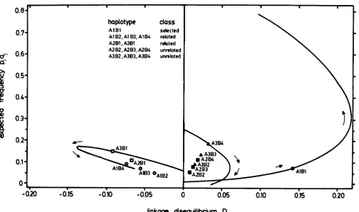
, s) are proportional to the A, and E, frequencies, but the normalized disequilibrium values will often not be equal, depending on the allele frequencies.

These features are illustrated in Figures 1 and 2, which give plots of the linkage disequilibria, and normalized linkage disequilibria values, respectively, from the iterations of a selection model. T h e model considers three alleles at the A locus, and four alleles at the B locus, giving 12 haplotypes in the population. T h e vertical axis is P A , q B I , the expected frequency of

(3)

625

0. e

0.7

e-

0.6

a-

p

0.5

2

0.4

r

P 0

H

0.3

0.2

0.1

0.

8

I 1 1

haplotype

class

A1 81 selected

A1 8 2 , A1 83, A1 8 4 related

A2B1, A3B1 rebted

A282, A2B3, A284 unrebted A382.A383. A384 unrehted

-

I 1 I

20 -

0.15

-

0.m

-

0.05

0

0.05 0.10 015 0.20

linkage disequilibrium D

# AlBl

r I I I I 1 I I

20 -

0.15

-

0.m

-

0.05

0

0.05 0.10 015 0.20

linkage disequilibrium D

FIGURE 1.-Results of a deterministic two-locus selection model having three and four alleles at each locus, showing the linkage disequilibrium, D, of the twelve haplotypes during directional selection (selection coefficient 0.5) favoring the AIBl haplotype. The initial generation is in linkage equilibrium (all haplotypes at D = 0). The trajectory of one haplotype from each class is shown through 25 generations. The location of each haplotype at generation eight is indicated. The initial frequencies for the alleles A I , A2 and A3 are 0.03,

0.37 and 0.60, respectively, and for the alleles E l , Ep, BS and B4 are 0.10, 0.20,0.30 and 0.40.

the haplotype if there is no linkage disequilibrium. This choice of axis allows easy discrimination between haplotypes with low and high frequency alleles, and permits easy identification of the proportionality of the negative linkage disequilibrium values with the frequency of the unshared allele. The model is strictly deterministic in that the effects of drift are not considered. Selection favors one haplotype, A I B I , and we consider directional selection with a selection coefficient of 0.5 applied to all genotypes lacking the favored haplotype. A large selection coefficient was chosen in order to observe rapid movement of h a p lotypes in the disequilibrium space: the results are not qualitatively different when other selection values are used. Initial allele frequencies were chosen to differ, the initial disequilibrium values of all haplotypes were zero, and recombination was zero. The favored haplotype was started at a low frequency.

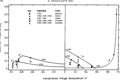
The increase and then decrease in the value of the linkage disequilibrium D for the A I B l haplotype with time (Figure 1) relates to the fact that the maximum value that D can take is a function of the allele frequencies. Note that the normalized linkage disequilibrium D’ increases over time (Figure 2).

The linkage disequilibria of each of the classes of related haplotypes, that is (A1B2, A I B ~ , and AlB4) and

(A2BI and A s B l ) , respectively, form a line in the neg-

ative space passing through the point D = 0, p q = 0 in the D space (Figure 1) and each set of related haplotypes assumes a single

D

value (Figure

2).

Un- related haplotypes (A2B2, A2B3, A2B4 and A&, A&, A3B4) fall on a line in the D space but form more complicated alignments in the D’ space because the value of

D,,,

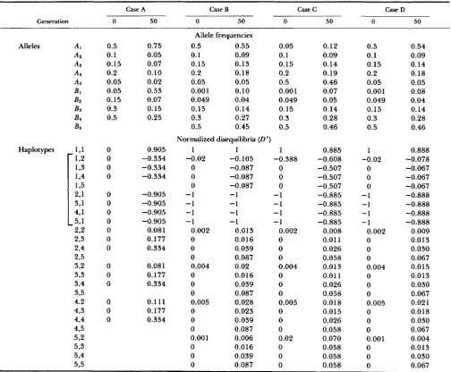
varies with the relative allele frequencies (see APPENDIX).

These results are also illustrated in case A of Table 1 where the frequencies of five alleles at the A locus and four alleles at the B locus, and the normalized linkage disequilibria (D’) of all the pairwise combinations of alleles, are given at generations 0 and 50. All initial disequilibrium values are zero, the selection coefficient of the A I B l haplotype is 0.1

,

and we assume no recombination. At generation 50 the related haplotypes have DC ( j =

2 ,

. .

. ,

4) values which are all equal to -0.334, and Di;

(i

=

2,

. . .

,

5 ) values which are all equal to -0.905. The normalized disequilibrium of the A I B I haplotype has a value of 0.905 which equals the larger in absolute value of the normalized disequilibria of the related haplotypes. The positive disequilibria of the AiBj haplotypes

(i

=

2,

. . .

, 5 ; j =

2,

. .

.

, 4) assume a number of different normalized values, depending on the relative frequencies of the constituent alleles.

(4)

G.

0.6 O . 1

0.54

0.4-

0.3-

key

haplotype

class

A l B l setected

0 A182, A193, AlBZ related

0 A 2 B 1 ~ A3Bl related

AZB2,A2B3, A2BZ unrelated

1, A382, A383, A384 unrelated

Y

.

I I

-1:o

-0.8

-

0.6 -

0.4 -

0.2 .

1 1

0.2

0.4

0.6

0.8

1

standardized linkage disequilibrium D'

FIGURE 2.-Deterministic selection model identical to that in Figure 1, plotted against standardized linkage disequilibrium D'. The location of haplotypes at the 8th and 16th generations is indicated, with the trajectories over 25 generations shown for the selected haplotype, one from each of the related classes of haplotypes and one from each of the unselected classes.

A , or B , , say R I , is a new mutant and forms the haplotype AIBl from the haplotype A1B2, and the haplotype AIRl is selected, the same basic results out- lined above continue to apply, if we assume zero linkage disequilibrium before the new mutant arose. One exception to the general results .is that for the related haplotype bearing the allele from which the new mutant arose, Die(n) will be larger in absolute value than the value of D i j ( n ) ( j = 3,

. . .

, s), where n is the number of generations since the new mutation arose (and hence since selection has been operating), {see cases B , C and

D

in Table 1). The occurrence of the new mutant creates nonzero linkage disequilibrium for a number of other haplotypes (see equations

(1-1 5a)-(I-l se), and cases B, C and D of Table 1). One point of specific interest is that the

D:,

(i

= 2,

. .

.

, r )

values will all equal

-

1 initially, and will maintain this value if recombination is zero (see case B of Table I). 'The case of nonzero recombination has been considered by computer iteration of various deterministic selection models (see APPENDIX and Table 1). The

results obtained for the case of zero recombination all continue to apply with recombination. Two examples where BI is a new mutant forming the haplotype A$, from the haplotype A&, with recombination R =

0.01 and selection coefficient 0.10 for the haplotype

AIBl are given in Table 1. In case C , the alleles A I and

B2 are both relatively rare, while in case D , A , is

common and B2 is rare (case

D

i s the same as case B ,

except for the recombination values). With nonzero recombination the L):,(i =

2,

. .

.

, r ) values decay from their initial value of -1. (Note that for a hitchhiking event to be important in influencing allele frequencies and linkage disequilibrium values we require that the selection intensity exceed the recombination fraction

(s

>

R ) (THOMSON 1977; ASMUSSEN and CLEGG 1981; ASMUSSEN 1986), and a similar constraint probably obtains for direct selection.)

When one haplotype is favored, as in our model, a total of T

+

s

-

2

related haplotypes (haplotypes having

an allele in common with the selected haplotype) move into the negative space, while the remainder ( r

-

1)(s

-

1) of haplotypes, that is, all those haplotypes unrelated to the selected haplotype, move into the positive space. If selection is operating on

X

haplotypes con- currently, and these haplotypes do not share any alleles, we expect X ( r i- s)

-

2(1

+

2

-t

.

,

+

K)

(5)

TABLE 1

Allele frequencies and normalized linkage disequilibria

Case A Case B Case C Case D

Generation 0 50 0 50 0 50 0 50

0.5 0.1 0.15 0.2 0.05 0.05 0.15 0.3 0.5 0 0 0 0 0 0 0 0 0 0 0 0 0 0 0 0 0 0.75 0.05 0.07 0.10 0.02 0.53 0.07 0.15 0.25 0.905 -0.334 -0.334 -0.334 -0.905 -0.905 -0.905 -0.905 0.081 0.177 0.334 0.08 1 0.177 0.334 0.1 11 0.177 0.334 Allele frequencies

0.5 0.55

0.1 0.09

0.15 0.13

0.2 0.18

0.05 0.05

0.001 0.10

0.049 0.04

0.15 0.14

0.3 0.27

0.5 0.45

Normalized disequilibria (D’)

0.05 0.1 0.15 0.2 0.5 0.001 0.049 0.15 0.3 0.5 1 -0.02 0 0 0 -1 -1 -1 -1 0.002 0 0 0 0.004 0 0 0 0.005 0 0 0 0.001 0 0 0 1 -0.105 -0.087 -0.087 -0.087 -1 -1 -1 -1 0.013 0.016 0.039 0.087 0.02 0.016 0.039 0.087 0.028 0.023 0.039 0.087 0.006 0.016 0.039 0.087 1 0 0 0 -1 -1 -1 -1 0.002 0 0 0 0.004 0 0 0 0.005 0 0 0 0.02 0 0 0 -0.388 0.12 0.09 0.14 0.19 0.46 0.07 0.05 0.14 0.28 0.46 0.885 -0.608 -0.507 -0.507 -0.507 -0.885 -0.885 -0.885 -0.885 0.008 0.01 1 0.026 0.058 0.013 0.01 1 0.026 0.058 0.018 0.015 0.026 0.058 0.070 0.058 0.058 0.058 0.5 0.1 0.15 0.2 0.05 0.001 0.049 0.15 0.3 0.5 1 -0.02 0 0 0 -1 -1 -1 -1 0.002 0 0 0 0.004 0 0 0 0.005 0 0 0 0.001 0 0 0 0.54 0.09 0.14 0.18 0.05 0.08 0.04 0.14 0.28 0.46 0.888 -0.078 -0.067 -0.067 -0.067 -0.888 -0.888 -0.888 -0.888 0.009 0.013 0.030 0.067 0.015 0.013 0.030 0.067 0.02 1 0.018 0.030 0.067 0.004 0.013 0.030 0.067

Allele frequencies and normalized linkage disequilibria (D’) are presented at generations 0 and 50 with selection coefficient 0.1 (dominant directional selection) for the A I B l haplotype under four contrasting conditions: Case A, all initial disequilibrium values zero and no recombination (R = 0); Case B, BI is a new mutant on haplotype AlBt which arose from haplotype AlBs with AI common and B2 rare, R = 0; Case C, B I is a new mutant on haplotype AlB1 which arose from haplotype AlBz and A I and B2 are relatively rare, R = 0.01; Case D, as for Case B with R = 0.01. Related haplotypesare bracketed.

thus give an indication of the minimum number of selection events which are acting, or have acted, on the system.

Neutrality: When mutation creates a new allele at a locus in a population, a new and unique haplotype is formed. This new haplotype will have the maximum positive D’ value, 1.0, all related haplotypes with the new mutant allele will be absent and so have D

’

values of

-

1 .O, while the linkage disequilibrium of the other related haplotypes with the non-mutant allele will be unaltered from their original value, except for the haplotype from which the new mutant derives (see equations (1-15a)-(I-l5e) in APPENDIX). If the new haplotype persists in the population and increases in frequency, recombination will generate new related

haplotypes in numbers proportional to the frequencies of the alleles at the unmutated locus. It is possible to imagine that genetic drift and mutation alone can produce the same pattern in the disequilibrium space as the selection models described above. Initially, the related haplotypes which have the new mutant allele have disequilibrium values which are maximized and proportional to the frequency of the unshared allele, and identical normalized disequilibrium values, equal- ing

-

1. Is the pattern generated by a selection event mimicked as recombination and genetic drift operate to reduce the disequilibrium values from their maximum?

(6)

628

terns generated in a two locus neutrality model. We generated data samples of size 10,000 for 4Nc values of 0, 1, 10, 25, 50, 75, 100, 160 and 500, where N is the effective population size and c is the amount of recombination between loci. (The rarer alleles were combined into one allele class to mimic the undefined “blank” alleles found in HLA data.) We chose 0 =

4 N p , where is the mutation rate, so as to generate samples with large numbers of alleles, close to the 13 alleles at one locus and 21 at the other as seen for the HLA data analyzed in the companion paper KLITZ and THOMSON (1 987).) Once the normalized disequilibrium values move away from the D‘ = -1 region the pattern generated by a selection event is not mimicked. A very wide range of normalized linkage disequilibrium values was observed and the approxi- mate constancy of normalized linkage disequilibrium values of each set of related haplotypes in the negative disequilibrium space, as predicted by the selection model, is not found in the neutrality case once recombination starts to reduce the initial

D ’

= -1 values.

At this stage we have no objective method for determining if a population sample fits the selection pattern or not. T h e patterns we have described as indicative of selection were arrived at by considering a completely deterministic model. Sampling variance will always cause some deviations from the deterministic predictions. At this exploratory phase of data analysis we have erred on the conservative side and make no statement about data sets which are neither very close to nor very far from the selection predictions. We are currently investigating various ap- proaches to statistical testing.

Migration or continuous admixture: If sizeable differences in allele frequencies exist between two populations, then large amounts of linkage disequilibrium can be generated by migration or admixture (see for example, NEI and LI 1973, FELDMAN and CHRIS-

TIANSEN 1975, THOMSON, BODMER and BODMER

1976). However, except in a very limited set of cases, the pattern of disequilibrium that will be generated by migration o r admixture is very different from the specific pattern predicted in the case of selection. This is demonstrated theoretically by considering the stan- dard static model of migration where two populations are mixed in proportions m and 1

-

m , and the case of continuous admixture of the two populations, and then by computer iteration of general migration models.

Consider a two locus, multiallelic model and let the frequency of the allele A, at the first locus be

p ,

in population 1, and P, in population 2, for

i

= 1,

. .

.

, r . Similarly, let the frequency of the allele B, at the second locus be q, in population 1, and Q J in population 2, f o r j = 1,

. . .

, s. In the static mixed population the linkage disequilibrium D,J between the alleles A,

and EJ is given by

D, = mDf f (1

-

m)D;

+

m(l

-

m > (P,

-

()Z‘ qJ

-

Q J ) ( 5 4

i =

1,

. . . ,

r ;

j =

1,

. . . ,

s,

where 0; and D ; denote the linkage disequilibria in the two populations considered separately (see CAV- ALLI-SFORZA and BODMER 197 1, page 69). If there is no linkage disequilibrium in each population initially, that is

Di

= D: = 0, then

(5b)

Dij = m ( l

-

m)(pi

-

Pz)(

91

-

QI)

i =

1 ,

. . . ,

r ; j = 1,

. . . ,

s,

so that, D, # 0 even if DE: = D ; = 0, provided the allele frequencies in the two populations are different. Take the case of admixture of say population

2

into population 1 (THOMSON, BODMER and BODMER 1976), where a proportion a of matings each generation involve an individual from population 1 with an individual from population 2, with the progeny entering population 1. If the disequilibria in the two populations are initially zero, then, at generation n the disequilibria in the admixed population are given by

i =

1, . . . , r ; j = 1

, . . . ,

s

where

and R is the recombination fraction between the A and B loci.

T h e only case of migration or admixture which can mimic the selection pattern with say the haplotype AIBl having high positive linkage disequilibrium and all related haplotypes at both loci having negative disequilibria proportional to the frequency of the unshared allele is the very restrictive situation where alleles A1 and BI are both more frequent in population 1 than population

2,

or vice versa, and all other alleles are rarer in population 1 than population 2, or vice versa. We assume that there is no linkage disequilibrium between any pairs of alleles in each population initially. In the static mixed population, and in the continuously admixed population for this example, alleles A1 and B1 will be in positive linkage disequilibrium, while all combinations of A I with non B , alleles, and B , with non A , alleles, will be in the negative linkage disequilibrium space. T h e frequencies of the

(7)

where m, = m in the static migration model and m, = [ 1

-

(a/2)]" in the admixture model. T h e haplotypes in the negative disequilibrium space, say for example

A 1 with all non-B1 alleles, will only have linkage disequilibrium values proportional to the Bj, j = 2 ,

. . .

,

s, frequency in the mixed population (the selection expectation) if

-B(fl1

-

Pl)(qj

-

Q j ) = P[m,qj

+

(1

-

mn)Q13,

j = 2 ,

. . . ,

s ,

where B = m ( l

-

m ) in the static migration model, and B = A in the admixture model and /3

>

0, that is if

- ( q j

-

Q j ) = Y[mnqj

+

( 1

-

m n ) Q j ] j = 2,

. . .

, S,

where y = P/B(fll

-

P I )

>

0, that is, only under the very stringent condition that for a l l j = 2 ,

. . .

, s

Thus, the situation where the selection pattern will be mimicked by migration occurs only under the most unlikely situation of a strict proportionality of the non-AI, non-BI alleles in the two populations, and also that both A l and B 1 are more frequent in one population than the other, and that all the other alleles in that population are all rarer. A simple case of this type would be if the haplotype A I B l is fixed in one of the populations. We have shown by computer iteration that this same exact result applies for continual migration occuring each generation between two populations. In general, the patterns of linkage disequilibrium generated by migration will differ greatly from the selection expectations.

DISCUSSION AND SUMMARY

Disequilibrium pattern analysis is a general method useful for revealing the evolutionary dynamics of tightly linked highly polymorphic loci in natural populations. Recent selection events can be identified from the pattern of the array of two-locus haplotypes in the disequilibrium space subdivided on the basis of all haplotypes sharing one allele. T h e pattern of haplotypes generated by a selection event is distinct from those produced by migration or random genetic drift. T h e analysis assumes zero linkage disequilibrium initially for all haplotypes, before the onset of the selection event. T h e distinct pattern of linkage disequilibrium values generated by a selection event holds for all generations while the selection is acting. This pattern will also presumably be maintained for many generations after the selection event, until the disequilibrium pattern is broken down by recombination and genetic drift. T h e same basic results continue to apply if the selection involves a new mutant, if we

assume zero linkage disequilibrium before the new mutant arose.

In particular, the following criteria are used to reveal selection, and specifically to identify those two- locus haplotypes showing the effect of selection, and thereby differentiated from other haplotypes in the population: (i) the magnitude of the expected frequency and D values of those haplotypes having positive disequilibrium values, (ii) the presence ofjust one o r a few haplotypes in the positive disequilibrium space when we plot the linkage disequilibrium for all haplotypes containing a given allele, and (iii) related haplotypes sharing an allele with a selected haplotype assume a value of linkage disequilibrium, D , proportional to the frequency of the unshared allele and have a common negative value of D ' .

In addition, the distribution of the number of haplotypes having positive and negative disequilibrium values can be used to predict the minimum number of recent haplotypic or hitchhiking selection events occurring in a region. T h e less common of the two alleles in a selected two locus haplotype will have arisen more recently. This conclusion is substantiated by the presence of fewer haplotypes with positive

D

values in the graph of the linkage disequilibrium values for all the haplotypes with the rarer allele. T h e disequilibrium pattern based on the rare allele will be the most sensitive in revealing the selective event, as the pattern based on the more common allele will also carry evidence of its previous history.

Disequilibrium pattern analysis is particularly per- tinent to the analysis of data from multigene families, marker trait associations and restriction fragment length polymorphism data. T h e close linkage of a number of loci in the HLA region, and the high level of polymorphism exhibited by many of these loci make it ideally suited for the study of evolutionary forces by disequilibrium pattern analysis. T h e companion paper (KLITZ and THOMSON 1987) analyzes a large sample of two-locus HLA data in this fashion.

We thank R. HUDSON for the use of his elegant simulation program and P. HEDRICK for his helpful comments on the manu- script. This research was supported by National Institutes of Health grants HD12731 and GM35326 and a UC Berkeley IBM Academic Information Systems grant.

LITERATURE CITED

ALBERT, E., M. BAUR and W. MAYR (Editors), 1984 Histocom- patibility Testing 1984. Springer-Verlag, Berlin.

ASMUSSEN, M. A., 1986 The dynamics of interlocus associations in the three locus hitchhiking model. 2. The pairwise linkage disequilibrium between two neutral loci. J. Math. Biol. 23: 285-304.

Dynamicsof the linkage disequilibrium function under models of gene-frequency hitch- hiking. Genetics 99: 337-356.

BAUR, M. P. and D. GRANGE, 1983 Negative linkage disequilibria. Tissue Antigens 21: 262-263.

(8)

CAVALLI-SFORZA, L. L. and W. F. BODMER, 1971 The Genetics of

Human Populations. W. H. Freeman, San Francisco.

DAUSSET, J. and P. J. COLOMBANI (Editors), 1973 Histocompatibility Testing 1972. Munksgaard, Copenhagen.

FELDMAN, M. and F. B. CHRISTIANSEN, 1975 The effect of population subdivision on two loci without selection. Genet. Res.

24: 151-162.

HANSEN, H. E., S. 0. LARSEN, L. P. RYDER and L. S. NIELSON, 1979 HLA-A,B haplotype frequencies in 5,202 unrelated Danes by a maximum-likelihood method of gene counting. Tissue Antigens 13: 143-153.

Properties of a neutral allele model with intragenic recombination. Theor. Popul. Biol. 23: 183-201.

Disequilibrium pattern analysis. 11. Application to Danish HLA-A and B locus data. Genetics

1 1 6 633-643.

LEWONTIN, R. C., 1964 The interaction of selection and linkage.

I. General considerations; heterotic models. Genetics 4 9 49- 67.

NEI, M. and W-H. LI, 1973 Linkage disequilibrium in subdivided populations. Genetics 75: 213-2 19.

TERASAKI, P. (Editor), 1980 Histocompatibility Testing 1980. Uni- versity of California, Los Angeles.

THOMSON, G., 1977 The effect of a selected locus on linked neutral loci. Genetics 85: 753-788.

THOMSON, G., W. F. BODMER and J. BODMER, 1976 The HL-A system as a model for studying the interaction between selection, migration and linkage. pp. 456-498. In: Population Ge- netics and Ecology, Edited by S. KARLIN and E. NEVO. Academic Press, New York.

Communicating editor: W. J. EWENS HUDSON, R. R., 1983

KLITZ, W. and G. THOMSON, 1987

APPENDIX

For generality and realism w e consider a hitchhiking model, where selection is considered not to be acting directly on the alleles A, (i = 1, . .

.

, r) and BJ (j = 1,

. . .

, s) of the A and B loci, but on a third linked locus where a new selected mutant F has arisen on an AIBl bearing haplotype. We denote the frequency of the AlBl haplotype which carries F by yl and the frequencies of all the other haplotypesA,BJ ( i = 1,

. . .

, r ; j = 1,

.

. . , s), which carry the alternate allele f by xy, with y l l

+

E:=,

xg = 1. We denote the allele frequency of A I by p ~ ~ , off by pf, etc. At this stage we assume zero recombination. (Note that the results we obtain below also apply if selection is acting directly on the haplotype AIBI).

The selection acting is assumed to be heterozygote advantage (although the results obtained below apply equally to directional or frequency dependent selection), with the following fitness values,

If haplotype frequencies in the next generation are denoted by primes ('), then

(I-2a)

(i = 1, . . . , r; j = 1,

.

. . , s), where

ui = 1

-

S y L

-

t ( l

-

yI1)2.

From (1-2b), we can write

x; 1 - t(l

-

y l l )

- -

-

Xy W

and using (1-2a) and (I-2c), this can be written as

(I-2c)

If haplotype frequencies at generation n are denoted by yl ] ( n )

and x,,(n), then it follows from (1-3) that

x& 1

-

y11(n)

-

p&)

XJO) - 1

-

Y I l ( 0 ) P/(O)'

(i = 1, . . . , r; j = 1,

.

. . , s). Also, from (I-4),

(1-5)

(i = 2 , . . . , r ; j = 2,

.

. . , s).

generation n by D,(n), and from equation (I),

We define the linkage disequilibrium between alleles A, and E, at

=

%dn)

-

p A , ( n ) p B , ( n ) (1-6)

(z = 1,

. . .

, r; j = 1,

.

. . , s; except i = j = 1). We denote the change in allele frequencies by

sA,(n) = P A L n )

-

p A , ( o ) (I-7a)

and

= P E A n )

-

p B J ( 0 ) . (I-7b)

Using (1-4) and (1-5) in (1-6) we obtain

DIJjn) =

-

p.41(n)pii,(n)

( j = 2, .

.

. , s). Similarly

(I-8b)

( i = 2, . .

.

, r).

Using equation (2), and (I-sa) and (I-8b) gives,

and

(I-9c)

(I-9d)

( 2 = 2 , . .

.

, r ; j = 2,

. . .

, s).

If the disequilibrium between A I and B1 at the start of the selection event is zero, or positive, then D I ~ ( n ) will always be positive, similarly for all the De(n) (i = 2,

.

. . , r ; j = 2,

. . .

, s) terms, since

aAI(n) and as,(.) are positive, and 6 A , ( n ) (i = 2, . . . , r) and &,(n) ( j =

2,

. . .

, s) are negative. The disequilibrium terms for the haplotypes containing only one of the alleles, A1 or E l , of the related haplotypes, that is Dl,(n)(i = 2,

. .

. , s), and &(n)(i = 2, .

. .

, r) will all similarly be negative.

(9)

tive disequilibria of the related haplotypes AI with the 4 ’ s (J # 1) are all proportional to the present B, frequency, if the initial disequilibrium values are zero, that is, D,(O) = 0, f o r j = 2,

. .

. , s (from I-Sa),

Di,(n) = -fl~~(n)&+,(n). (I-loa) Similarly, the negative disequilibria of the related haplotypes BI

with the A,’s (t # 1) are all proportional to the present A, frequency, if the initial disequilibrium values are zero, that is, D,l(O) = 0, for i

= 2,

. . .

, r (from I-Sb),

D,l(n) = -fA,(n)&i~(n). (I-lob) For polymorphic loci where PA,

+

PE, 5 1 (j = 2,

.

. . , s) (BAUR

and GRANGE 1983) as is usually the case, for the negative D , values Dl,(max) = P A , & (see equations (4d)-(4e)), and similarly for the negative D,l value, D,l(max) = Thus if the initial disequilib-

rium values are zero, the normalized disequilibrium values D i,(n) and Dil(n) are

0’ = 2,

.

. . , s), and

(1-1 la)

(1-1 lb)

(i = 2, .

. .

, r). The expected DIj(n) values are equal for all j = 2, . ,

.

, s, and similarly the Dh(n) values each have the same expectation for i = 2,

. . .

, r . (These results for D;j(n) and Dh(n) do not hold if

P A ,

+

P E j > 1 or P A i

+

PEI > 1, respectively.)

If Dll(0) = 0 and P A , < $ E , , then

while if PA, > PE,, then

(I-12a)

(I-12b)

The positive disequilibria of the unrelated haplotypes A, and B,(i = 2,

. . .

, r, j = 2,

.

. . , s) are proportional to the A, and B,

frequencies, if the initial disequilibria values are zero (from (I-9c) and (I-9d)),

D d n ) =

-PB,W&)

(I-13a)

= -P~dn)a~~(n) (I-13b)

If PA, PE,, then

and if PA, > #BJ, then

(I- 1 4a)

(I- 14b)

The normalized disequilibrium values for haplotypes with a particular allele A, with all alleles B,, j = 2, .

. .

, s, will not usually be equal, depending on the relative allele frequencies. Note that for highly polymorphic systems such as HLA, with a fairly even distribution of allele frequencies, DG(n) will be considerably less in value than oil(%), since 6 ~ , ( n ) will be larger than - S B , ( ~ ) , and pAl(n) will be smaller than 1

-

#E,@) (see (I-12a) and (I-14a) for example).

Case (b). The case where B1 is a new mutant: We now consider the case where we suppose that B 1 is a newly arisen mutant which forms the haplotype AIBl from the haplotype AI&, and that the haplotype AlBl is selected. The occurrence of the new mutant creates linkage disequilibrium. For comparison with the results

abbve, we assume that before the new mutant arises all pairwise disequilibrium values are zero. T h e linkage disequilibrium values created by the occurrence of the new mutant are as follows:

(I-15a)

(I-15e)

and all other linkage disequilibrium values zero (hence all the normalized values).

T h e D,l(n), i = 2, . . . , r, values still stay proportional to the current A, allele frequencies, with

D,l(n) = - P A d n ) f i B l ( n ) , (1-16)

and this should be compared with (I-lob). In this case D,’l(n) = -1, as recombination is assumed zero. Iterations of deterministic selection models with recombination, show that the linkage disequilibrium and normalized values with recombination yield the same general results obtained above for the case of no recombination. That is, the D,l(n) values are proportional to the A, allele frequencies and the D,’l(n) values are all equal.

For the AtB, haplotypes, excluding A&, that is j = 3,

. . .

, s, the initial linkage disequilibrium values are all zero (hence also the normalized values) and all the results obtained above for the proportionality of the disequilibrium values and equality of the normalized values for the case of zero initial disequilibrium continue

to apply. T h e haplotype AlB2 from which the mutant arose, will show a different pattern, as the initial disequilibrium (and normalized disequilibrium) are nonzero. If the frequencies of A I and B2 are reasonably large relative to the frequency of the new mutant B I

(so that D;2(0) is small) the DI&) and D;&) values will not deviate greatly from the case when all the initial disequilibrium values are zero. However, if the new mutant arises on a relatively rare haplotype, then D;z(O) will be a large negative value, and the values of

DI2(n) and Die(%) may deviate considerably from the patterns of

Dl,(n) and D;,(n), especially in the initial generations of selection.

Case (c). The effects of recombination: The general equations to determine haplotype frequencies in the next generation (x;),

given haplotype frequencies in this generation ( x ~ ) , fitness parame- ters wvkl for individuals of genotype X+U, (i, k = 1,

. . .

, r; j , 1 = 1,

. . .

, s) and recombination R between the A and B loci are

where

, S I . #

5 = W,jUxy%i. (I-17b)

,-I ,-I &-I 1-1

(10)

= xii(1

+

S) - R [(I

+

S X I I ) D11 Gx; = xs[l

+

s(1 - R)XII]

-

RD,, i = 2 , . . . , r;

(I-18a) (I-18d)

j = 2, . . . , s,

+

-

AI)

-

~ B I ) ]

$xiJ = X i J [ l

+

~ ( l - R)XII]

-

R(DI, - S X I I ~ , ) , where (I- 18b)

j = 2 ,

...,

s,

w

= 1

+

2 S X l I

-

sx:,. (1-1 8e)

Iteration of deterministic selection models with recombination shows that all the results obtained above still apply.

(1-1

sC)

Gx:~ = x,l[l

+

~ ( l

-

R ) x I ~ ]

-

R(Dzi - SXII~A,),