Dependent DNA Binding by SA1 and SA2. (Under the direction of Dr. Hong Wang).
Single-molecule interactions between proteins and DNA can reveal information about biological function that is difficult to obtain using bulk assay methods. Sister chromatid cohesion is mediated by the cohesin complex, which also plays important roles in diverse biological processes including maintenance of 3-D chromatin organization, DNA replication fork restart, and DNA double-strand break repair. In vertebrates, the core cohesin complex consists of a tripartite ring assembled from Smc1, Smc3, Rad21, and the stromal antigen subunit (SA) SA1 or SA2. All current models attribute cohesin DNA binding exclusively to the entrapment of ds-DNA by the cohesin ring subunits. In this thesis, we use
by
Preston James Countryman
A thesis submitted to the Graduate Faculty of North Carolina State University
in partial fulfillment of the requirements for the degree of
Doctor of Philosophy
Physics
Raleigh, North Carolina 2016
APPROVED BY:
_______________________________ _______________________________
Dr. Hong Wang Dr. Robert Riehn
Committee Chair
_______________________________ _______________________________
BIOGRAPHY
Preston James Countryman was born on November 22, 1986 in Daly City, California to Patricia Ellen Countryman and Preston Otis Countryman. He spent his adolescence living in the Bay Area, and moved to Sacramento at the age of 10. By 2004 he had enrolled at
ACKNOWLEDGMENTS
Committee members: Hong Wang, (NC State, Physics), Robert Riehn (NC State, Physics), Keith Weninger (NC State, Physics), Guozhuo Xu (NC State, Biochemistry)
Wang Lab: Jiangguo Lin, Parminder Kaur, Hai Pan, Dianwen Wang, Xuechun Wang, Christian White, Wang Miao
Collaborators: Ingrid Tessmer, Patricia Opresko, Susan Smith, Neil M. Kad, Jacob Piehler, Yizhi Jane Tao
TABLE OF CONTENTS
LIST OF FIGURES ... vii
Introduction ... 1
CHAPTER 1: Fundamentals of atomic force microscopy ... 5
1.1 Introduction ... 5
1.2 Atomic Force Microscopy (AFM) ... 5
Modes of operation ... 6
Sample preparation for AFM imaging ... 8
AFM imaging in liquids ... 10
Force analysis using AFM ... 11
Imaging improvements ... 12
AFM studies of protein-protein and protein-DNA interaction ... 13
Data processing of AFM images... 15
CHAPTER 2: Fundamentals of fluorescence microscopy ... 18
2.1 Introduction ... 18
2.2 Theory behind TIRF ... 18
2.3 Penetration depth and Oblique Angle Fluorescence ... 20
2.4 Single molecule tracking... 21
2.5 Quantum dot properties and fluorescent dyes ... 27
2.6 Protein-QD conjugation methods ... 28
2.7 Gap DNA preparation ... 29
2.8 Specifications of in lab fluorescence microscope ... 30
CHAPTER 3: Single-particle tracking of quantum-dot labeled proteins on DNA ... 32
3.1 Introduction ... 32
3.2 Improved positional accuracy through Gaussian fitting ... 32
3.3 Methods of data analysis ... 33
3.4 Prediction of diffusion constants and stepping rates based on Stokes-Einstein relation ... 38
3.5 Prediction of additional energy barriers ... 40
4.1 Cohesin background... 42
4.2 Summary ... 43
CHAPTER 5: Functional interplay between SA1 and TRF1 in telomeric DNA binding and DNA-DNA pairing ... 53
5.1 Background ... 53
5.2 Summary ... 54
CHAPTER 6: Telomere maintenance pathway ... 62
6.1 Introduction to telomeres ... 62
6.2 Summary ... 67
Conclusion ... 78
REFERENCES ... 83
APPENDICES ... 101
Appendix A: Cohesin SA2 is a sequence independent DNA binding protein that recognizes DNA ends and gaps ... 102
Appendix B: Functional interplay between SA1 and TRF1 in telomeric DNA binding and DNA-DNA pairing... 141
LIST OF FIGURES
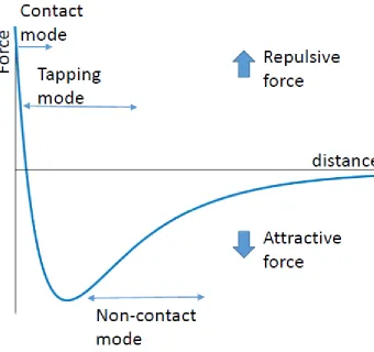
Figure 1: Cartoon representation of the principal mechanism behind AFM scanning ... 16 Figure 2: Example force vs distance curve that mirrors the type of interaction between the scanning tip and sample during AFM measurements using specific imaging modes ... 17 Figure 3: SA2 does not show binding preference for telomeric or contromeric DNA
sequences, but recognizes DNA ends. ... 46 Figure 4: SA2 specifically binds to ssDNA gaps... 48 Figure 5: SA2 switches between searching and recognition modes on DNA tightropes
Introduction
The modern notion of molecular biology is a convergence of various disciplines, including biochemistry, genetics, microbiology, and physics. The principal notion is to build a complete understanding of a system by starting at macromolecular properties of materials and examining their interactions. For most biological systems, the essential materials are nucleic acids (DNA or RNA), and proteins. The interactions between these two basic biological building blocks, as well as the machinery for their synthesis, repair, and
A variety of methods exist to isolate, identify, or examine the role of individual proteins, such as X-ray crystallography, electron microscopy, electrophoresis, and many others. X-ray crystallography pioneer Dorothy Crowfoot Hodgkin was awarded the Nobel Prize for Chemistry in 1964 for her work in solving the chemical structure of cholesterol, penicillin, and vitamin B12. Identification of the 3D structure of a compound is necessary to construct a working model for available chemical bonds and conformational configurations available for biological compounds (Scapin 2006). Transmission Electron Microscopy (TEM) passes a beam of electrons through a thin slice of an object and collects the transmitted electrons, which contain information about the material they have interacted with. This technique allows for higher resolution than light microscopes provide and greater magnification to observe the 3D structure of a biological compound (Harris 2015). However it requires extensive sample preparation and vacuum conditions for the sample in question, thus the information obtained may no longer be biologically relevant. Biological techniques such as electrophoresis allow for the isolation of proteins by charge or molecular weight, while western blotting isolates proteins using conjugation methods.
This dissertation focuses on examining the specific interactions of proteins using single-molecule techniques in environments similar to biological conditions in order to provide the scientific community with a more comprehensive understanding of their
respective biological systems. The first system is the shelterin protein complex present on the telomere portion of DNA. The shelterin complex is imperative for preventing the
DNA replication, and providing stability to t- and D-loop formation at DNA ends. However the shelterin complex is composed of 6 unique proteins and uses a variety of cofactors and ancillary proteins in order to execute the plurality of functions mentioned above. By using the single-molecule techniques of atomic force microscopy (AFM) and fluorescence methods, we showed that shelterin proteins TRF1 and TRF2 bind specifically to the
telomeric portion of DNA and diffuse along the DNA backbone in order to locate telomeric regions of DNA. These techniques elucidate how the shelterin complex protects DNA
through the primary interaction of TRF1 and TRF2 with DNA. The second system of interest was the cohesin complex, which regulates the segregation of sister chromatids during cellular replication and prevents the end joining of distant DNA strands. Like shelterin, each cohesin complex consists of 4 unique proteins and requires a bevy of cofactors and other proteins to perform its duty. We showed that cohesin protein SA2 by itself has a strong binding affinity to DNA ends and gaps, independent of the sequence of DNA. Single-molecule techniques allowed us to pinpoint a specific behavior for SA2 that fits a role for the cohesin complex, allowing further studies to target SA2 as the active DNA binding protein for the entire cohesin complex. We also found that cohesin protein SA1, which can replace the role of SA2, has an affinity for telomeric DNA sequences and this affinity is increased in the presence of telomere protein TRF1.
CHAPTER 1: Fundamentals of atomic force microscopy
1.1Introduction
Interactions between proteins and DNA are fundamental in diverse biological processes, including DNA repair, replication, and transcription (Billingsley, Bonass et al. 2012, Qiu, DeRocco et al. 2012, Stratmann and van Oijen 2014). Revealing the structure and dynamics behind protein-DNA interactions is the key to improving the understanding about these complex biological systems. Single-molecule studies can provide addition about population distributions lost in bulk biochemical assays that only report the average system behavior. Importantly, single-molecules techniques allow for the observation of biologically rare important events or conformations that are not reported in bulk assays. This work focuses on applying single-molecule atomic force microscopy (AFM) to investigate the conformational properties of the protein-DNA interactions involved in telomere maintenance pathways and sister chromatid cohesion.
1.2Atomic Force Microscopy (AFM)
physical properties of biological samples in air or liquids with high surface resolution (Bustamante and Rivetti 1996).
Modes of operation
AFM is a near-field approach, wherein a sample surface is directly probed by a sharp tip (several nanometers in diameter) attached to a flexible cantilever. A laser is reflected off the back of the cantilever into a four quadrant photodiode. During the scanning process, the cantilever is bent towards the surface due to attractive tip-surface interactions, or reflected away from the surface due to repulsive surface interactions. These interactions are captured by the deviation from the central location of the photodiode (Figure 1: Cartoon representation of the principal mechanism behind AFM scanning). The most commonly used AFM imaging modes include contact mode, intermittent contact mode (or oscillating mode), and
non-contact mode. The height profile is measured directly from the deviation of the reflected laser onto the four-quadrant photodiode with sub nanometer precision capability.
Contact mode requires constant direct contact between the AFM tip and the sample surface. The shear forces from the tip dragging over the surface increase the odds of damaging or moving individual protein and DNA molecules, which leads to sample
oscillations. The feedback loop keeps the amplitude of oscillation constant as the tip scans over the surface, whereas in contact mode the angle of cantilever deflection is what is held constant. The brief interaction between the tip and surface greatly reduces stress forces, allowing for superior imaging of protein and DNA systems (Bustamante and Rivetti 1996). In order to ensure proper imaging of the sample, the tip-sample distance needs to be held constant with sub-nanometer uncertainty. This is accomplished by using a frequency modulated signal to dampen external forces that affect the tip-sample distance (Martin, Williams et al. 1987, Rode, Oyabu et al. 2009).
A further development known as non-contact mode relies solely on attractive and repulsive forces between the surface and the tip without actually making contact with the sample, thus best preserving the integrity of the sample. These non-contact forces dampen the amplitude of oscillation, which is corrected by the feedback loop in order to keep the amplitude constant. This stress reduction makes tapping imaging the ideal candidate for imaging dense protein/DNA systems.
During scanning, AFM tip-sample interactions are mediated by combinations of forces including long-range electrostatic interactions, medium range attractive van der Waals forces (~10 nm), and short range repulsive Bohr forces (~0.1 nm) (Leite and Herrmann 2005). The repulsive Bohr force that dominates very close interactions occurs when two molecules begin overlapping electron orbitals, thus the repulsive force is a direct
𝑼 = 𝑪𝟏 𝒙𝟏𝟐−
𝑪𝟐 𝒙𝟔
(1)
where C1 and C2 are the corresponding constants of the repulsive and attractive forces
encountered by the tip and x represents the distance between the sample and tip. As the tip draws closer to the surface, it falls into the potential well, resulting in an attractive force on the tip (Figure 2: Example force vs distance curve that mirrors the type of interaction between the scanning tip and sample during AFM measurements using specific imaging modes). The attractive x-6 term is often described as the van der Waals interaction because it is the direct product of interaction between molecules on the tip and molecules on the surface (more on molecular interactions later). If the separation between the tip and sample continues to decrease, the repulsive x-12 term dominates, resulting in a net repulsive force on the tip (Leite Herrmann 2005).
AFM imaging of biological samples can be done either in air or in liquid. Liquid imaging is more complicated due to hydrodynamic interactions between the oscillating tip and the sample (Bustamante and Rivetti 1996). However the phase change between the cantilever vibration and the drive signal can be held constant via the feedback loop instead of the amplitude, which is called phase intermittent contact mode. Examining the phase
difference after sample interaction yields insight into the elasticity or friction of the sample. It has also been shown to improve resolution during liquid imaging of samples (Argaman, Golan et al. 1997).
An ideal surface for AFM imaging must be compatible with the sample and
exceptionally flat. While the latter issue is important to ensure that only the sample height is being measured, the former issue is much more important for biological samples. A variety of surfaces have been used to immobilize biomolecules, such as glass, silicon, and mica (Wagner 1998). Muscovite mica is the most commonly used substrate. It has a negatively charged surface that can easily be made atomically flat via a simple peeling process with household scotch tape. It is important to have cations such as Mg2+, Ni2+, or Ca2+ to act as salt bridges to adhere the negatively charged DNA or proteins to the mica surface (Hansma and Laney 1996). Another method is to chemically treat the mica surface to prepare a positively charged surface for depositing negatively charged samples without buffer limitations. For example, a silicon or mica surface incubated with
(3-aminopropyl)triethooxysilane (APTES) forms a self-assembled monolayer with siloxane bonds. The free, positively charged amino groups are then able to attach to negatively charged elements (Tessmer, Kaur et al. 2013).
without surface modification, ~20 ul of the sample is deposited on the surface, followed by a brief incubation time (< 30 seconds). The sample is then gently (to avoid striating the DNA on the surface) blown dry with nitrogen gas before being loaded onto the AFM.
AFM imaging in liquids
Liquid imaging offers the ability to observe real-time dynamics of biological systems while under physiologically relevant conditions. This can be for used for studying single-molecule systems, interactions between macrosingle-molecules, or live cells. Liquid imaging is particularly useful to analyze behavior of lipids for phase transitions or lipid mixtures
for ~250 nm scans to be completed in a few hundred milliseconds (Ando, Uchihashi et al. 2008). Improvements to the electronic circuits, cantilever deflection detection system, and other electronic circuits have also improved scanning speed (Ando 2012).
Force analysis using AFM
Another useful feature provided by an AFM is the ability to probe the physical interactions between biomolecular assemblies or cells using force spectroscopy. The
cantilever tip essentially acts as a spring that can test the force between the tip and the sample using Hooke’s Law
𝑭 = 𝒌 ∗ 𝒙 (2)
where F is the force measured by the tip deflection, k is the spring constant of the cantilever, and x is the displacement. The spring constant k can be calculated using
𝒌 = 𝒀𝒘𝒕
𝟑
𝟒𝑳𝟑
(3)
from which the force is then calculated (Zlatanova, Lindsay et al. 2000). Usually in Atomic Force Spectroscopy (AFS) experiments, the sample is immobilized on the surface while the interacting partner is adhered to the AFM tip. Analysis of a force versus distance curve can provide insight into the forces necessary to break or establish the bond between the two biological samples, examples of which include protein-protein interactions, DNA secondary structures, or ligand-receptor interactions (Lynch, Baker et al. 2009, Han, Qin et al. 2012, He, Hu et al. 2015). The force versus distance curve generated by this technique can also provide insight into intra-molecular forces.
Imaging improvements
There are many avenues of improvement for AFM technology to increase the
resolution of images. Perhaps the most obvious starting point is the tip used to scan over the sample. A tip with a smooth shape has some radius R near the apex of curvature. This tip curvature makes it difficult to resolve features between two objects on the surface located close to each other. The limit of resolution for the AFM tip depends on the distance between the surface objects (d), the height of the objects (h), the deformation height of the feature between objects (Δz), and finally R (Lyubchenko 2011). Tip sharpness is also a vital concern
with the sample or experiences an excess of force. Tips with [1 1 1] orientation proved more structurally stable due to increased bonding with surrounding tip molecules (Giessibl, Hembacher et al. 2000). Carbon nanotubes offer another suitable material for cantilever and tip construction. In addition to improved tip sharpness, carbon nanotubes have improved elasticity, which limits the maximum force it can deliver to biological samples (Wong, Joselevich et al. 1998). Controlling the length and orientation of carbon nanotubes is difficult however, thus the process of creating high quality tips from this method is expensive and tedious (Buchoux, Aime et al. 2009). Other factors that improve image resolution include tip-sample interactions, proper immobilization and adsorption on the surface of the tip-sample, pH balance of the buffer, and ionic strength of the buffer (Mou, Czajkowsky et al. 1995, Muller and Engel 1997, Muller, Fotiadis et al. 1999). Changes in temperature can cause the
cantilever to bend and possible alter the eigenfrequency of the tip (Giessibl 2003).
AFM studies of protein-protein and protein-DNA interaction
Due to the ease of sample preparation and low impact on biological samples, imaging protein-protein or protein-DNA interactions with AFM is an excellent way to examine single-molecule interactions in systems. As previously mentioned, on a mica surface, DNA molecules re-equilibrates on the surface in 2D, allowing for relevant information to be gathered from AFM images.
Proteins can also have a specific predilection for specific regions of DNA based on the sequence of DNA (Kaur, Wu et al. 2014, Lin, Countryman et al. 2014). Other proteins localize to regions of DNA damage, such as nicks, gaps, or breaks (Sukhanova, Abrakhi et al. 2016). Proteins can also serve as stabilizing agents for secondary DNA structures such as loops or G quadraplexes (Wang, Finzi et al. 2009). Analysis of protein position on DNA can yield information about the specificity of the protein to these regions, additionally providing the disassociation constant (Wang, Tessmer et al. 2008).
2. The size, shape, and volume of protein-DNA or protein-protein complexes.
In order to extract meaningful information from AFM scans, a volume calibration curve using known proteins can be used to create a linear relationship between volume measured by the AFM and the molecular weight of proteins (Wyman, Grotkopp et al. 1995, Ratcliff and Erie 2001, Yang, Wang et al. 2003, Sukhanova, Abrakhi et al. 2016). This relationship additionally allows for examination of protein aggregation and protein-DNA volume interactions (Daban 2011, Kaur, Wu et al. 2014). Additionally, the disassociation constants of proteins can be obtained from analysis of the AFM images (Ratcliff and Erie 2001, Yang, Wang et al. 2003).
3. The processing of DNA by proteins.
serve as a tool to investigate the effects of protein binding to DNA conformation, such as the DNA bending angle (Janicijevic, Sugasawa et al. 2003, Yang, Wang et al. 2003).
Recall that for all of these instances, the protein-DNA samples are held immobile on the surface. Thus the images generated by the AFM resemble instances in time rather than live, dynamic processes. Just like a movie, enough consecutive still images can give an idea for a larger pathway, process, or reaction. Each AFM scan takes a relatively small amount of time (on the order of minutes), making it possible to generate enough images to have a statistically robust sample size. Importantly, images from different depositions must be scanned and analyzed to avoid concluding results from sampling noise, deposition pollutants, or strange surface interactions. Additional controls, depending on the nature of the
experiment in question, are also necessary to avoid inclusion of artifacts into the data analysis.
Data processing of AFM images
A variety of platforms and programs exist, mostly generated by the scientific
community, to maximize the acquired data from each AFM scan. Many free programs, such as Gwyddion or ImageJ, can be used or customized in order to extract information such as height, area, volume, and length of AFM scans (both of which are used in our lab). More sophisticated and expensive software is necessary to analyze the complex interactions
many acceptable substitutes. Our lab uses Gwyddion to extract information such as height, area, volume, and length of DNA.
Figure 2: Example force vs distance curve that mirrors the type of interaction between the scanning tip and sample during AFM measurements using specific imaging modes
CHAPTER 2: Fundamentals of fluorescence microscopy
2.1Introduction
Over the years, Total Internal Reflection Fluorescence (TIRF) has become a staple of the biological community in order to examine a variety of systems under physiologically relevant conditions. Unlike AFM imaging in air, TIRF experiments provide dynamic information about the system in question. The highly adaptable system allows a plethora of samples, such as live cells, DNA suspended tightropes, and microtubules, to be viewed using fluorescent materials such as quantum dots or fluorescent dyes. The field is rapidly evolving, with revolutionary new adaptations of the basic technique altering the technical landscape nearly annually.
2.2 Theory behind TIRF
James Clerk Maxwell revolutionized modern science with his unification of light, electric fields, and magnetic fields. Previously these concepts were considered individually, but Maxwell was able to unify them in just four equations:
𝛁 ∙ 𝑫 = 𝝆𝒇 (4)
∇ × 𝑬 = −𝜕𝑩 𝜕𝑡
(5)
∇ ∙ 𝑩 = 0 (6)
∇ × 𝑯 = 𝑱𝑓+𝜕𝑫 𝜕𝑡
Armed with the fact that light is constructed of time varying electric and magnetic fields, Maxwell’s equations make it possible to establish boundary conditions for light as it
impinges on a surface:
𝒏
̂ ∙ (𝑫𝟐− 𝑫𝟏) = 𝝈𝒇 (8)
𝑛̂ × (𝑬2− 𝑬1) = 0 (9)
𝑛̂ ∙ (𝑩2− 𝑩1) = 0 (10)
𝑛̂ × (𝑯2− 𝑯1) = 𝑲𝑓 (11)
If there are no free charges on the surface and no surface currents, then equations (8-11) state that the normal components of D and B are continuous and the tangential components of E and H are continuous.
When a ray of light impinges on a surface, there are three total rays to ultimately consider: the initial ray, the reflected ray, and the transmitted (or refracted) ray. Snell’s Law (eq. 12) shows that the angle of the reflected ray with respect to the normal of the impinged surface is equal to that of the initial ray (although this can also be deduced by applying Maxwell’s boundary conditions).
𝜽𝒊= 𝜽𝒓 (12)
The transmitted light ray is governed by the law of refraction (eq. 13)
𝒏𝟏𝐬𝐢𝐧 𝜽𝟏= 𝒏𝟐𝐬𝐢𝐧 𝜽𝟐 (13)
where n is the index of refraction of the material the ray is moving through, and the
As θ1 increases, θ2 also increases, until the condition sin θ2 ≤ 1 is met. Thus a real angle for the transmitted light ray only exists for incoming light below a certain angle. This angel is defined as the critical angle
𝐬𝐢𝐧 𝜽𝒄 = 𝒏𝟐
𝒏𝟏 (14)
For angles greater than the critical angle, all light is reflected, which gives rise to total internal reflection. At the critical angle, the refracted light ray travels parallel to the surface. The refracted wave also has an amplitude that decreases perpendicular to the surface in material 2. This phenomena is known as an evanescent wave, and describes the decaying intensity of the light wave in the transmitted medium for incoming light at the critical angle. The amplitude of the evanescent wave decreases exponentially, and has a limited penetration depth (eq. 15) into the second medium
𝜹 = 𝟏 𝑲= (𝝀𝟐/𝟐𝝅) [(𝒏𝟏 𝒏𝟐) 𝟐 𝒔𝒊𝒏𝟐𝜽 𝒊− 𝟏]𝟏/𝟐 (15)
where λ2 = 2π/k2 = 2πc/n2w is the wavelength of a normal plane wave in the medium. Finally the application of Maxwell’s boundary conditions (8-11) reveals that the reflected wave has the same magnitude of electric field as the initial wave. Due to the conservation of energy between the initial and reflected wave, this is known as total reflection.
2.3 Penetration depth and Oblique Angle Fluorescence
bio-molecule (more on fluorescent devices later). In principal, a biological sample is placed on or close to a surface. A highly collimated light beam is incident on the opposite side of the sample at the critical angle, causing total internal reflection to occur. The evanescent waves allow for an energy transfer to the fluorescent devices to occur, but the penetration depth of the evanescent waves into the sample is limited. The typical penetration depth is on the order of hundreds of nanometers (Konopka and Bednarek 2008). While there are many adjustable parameters in order to determine the penetration depth of the evanescent wave (eq. 15), the angle of the incident laser beam has the most experimental variability. Oblique Angle Fluorescence (OAF) is a variant on the TIRF technique where sub-critical angles are used instead of the true critical angle. This technique generates an increased signal-to-noise ratio and increased penetration depth into the material (Kad, Wang et al. 2010). Furthermore, variable OAF studies allow for imaging of cells by mapping fluorescence as a function of penetration depth into the material by simply adjusting the sub-critical angle of the incoming beam (Konopka and Bednarek 2008).
2.4 Single molecule tracking
2010, Gorman, Wang et al. 2012, Wang, Redding et al. 2013). Breakthrough in the field of DNA repair have come about by examining intermediate protein-DNA interactions,
identifying motor proteins based on diffusion patterns, and extracting diffusion information from protein movement (Gorman, Chowdhury et al. 2007, Spies, Amitani et al. 2007, Gorman, Wang et al. 2012, Qi and Greene 2016).
Diffusion is a particularly interest problem of note. Many proteins are tasked with locating a specific DNA sequence or region along lengths of DNA many orders of magnitude longer than the location of interest. There are four diffusion methods utilized by proteins in order to search for targets: random three dimensional diffusion, 1D diffusion along the DNA substrate, 1D hopping in order to bypass obstacles, and intersegmental transfer (Berg, Winter et al. 1981, von Hippel and Berg 1989, Gorman and Greene 2008). Any searching
DNA to beads (Kad, Wang et al. 2010). First, poly-l-lysine is used to coat 5 micrometer silica beads. The coated beads are washed with a 20-fold excess of DI H20 and centrifuged twice at 16000G to wash the beads. They are then diluted in 100 microliters of DI H2O and
introduced into the flow cell for 5 minutes. The negatively charged oxygen of the carbonyl groups on the poly-L-lysine attract cations in the solution of the flow cell, which will ultimately create a salt bridge similar to that of the AFM in order to attract DNA. These beads are introduced into a closed flow cell at a concentration experimentally deduced to produce optimal coverage on the surface. Finally the beads are washed with the buffer used in the TIRF experiments to remove any weakly tethered beads.
The flowcell is constructed by drilling two holes 15 mm apart through a glass microscope slide. Plastic tubing is cut, expanded at one end using a heat gun, and pulled through the holes until taunt. The tubes are then glued into place using UV curing adhesive, which also seals any air pockets between the holes and tubing. Excess tubing is cleaved away using a box cutter. A coverslip is meanwhile prepared by thoroughly bleaching and cleaning. This is followed with amine functionalization with 3-aminopropyl-triethoxysilance in 2% dry acetone and washed thoroughly with DI H2O. Once the coverslips have been treated, they are sandwiched together along with PEG-SVA for ~4 hours before they are separated, washed, and dried. The coverslip is then attached to the glass slide with adhesive tape and sealed shut. Finally the flow cell is flushed with DI H2O.
to a 1.5 mL centrifuge tube that acts as a reservoir. The flow cell is again flushed with whatever imaging buffer is used for the experiment, taking precaution to avoid introducing air bubbles into the system. The DNA is then introduced into the system by injecting it into the reservoir and withdrawing the solution into the flow cell. Once inside the flow cell, the DNA is moved back and forth across the beads for ~15 minutes. The DNA sticks to the poly-L-lysine covered beads during this process, and continues in the direction of flow until it encounters another bead. If the DNA strikes another bead, it adheres again, creating a region between the two beads of taught DNA. The DNA remains taught even after the flow is shut off, allowing for observation under an absence of external flow.
In order to examine the stability and extension of DNA in the flow cell, it is necessary to evaluate DNA as an ideal polymer composed of N units with flexible linker ends allowing for random bend angles. In solution, each linker region is subject to thermal fluctuations, causing each bend angle to be a result of a random walk. The force required to extend the DNA must overcome the thermal fluctuations, and can be described according to the worm like chain model as follows
𝑭 = 𝒌𝑩𝑻 𝟒𝐀 ∙ ( 𝟏 𝟒 (𝟏 −𝒙𝑳)𝟐 −𝟏 𝟒+ 𝒙 𝑳) (16)
Bouchiat, Wang et al. 1999). These studies concluded that a force of 2-3 pN was sufficient to stretch ds DNA to ~90% of its contour length. The DNA can become overextended if ~60 pN forces are applied, and DNA has a theoretical breaking limit of ~500 pN. In the region
between 5-60 pN, the DNA stretches but maintains its integrity and helicity, thus it is essential to be within this regime for DNA within the flow cell. The force due to two dimensional laminar flow can be estimated using the following
𝒅𝒑
𝒅𝒙 = −𝟏𝟐𝒏 ∙ 𝑽 𝑩𝟐
(17)
where dp/dx is the pressure drop, n is the viscosity of the buffer in the flow cell, V is the velocity of the flow rate (flow rate divided by the cross sectional area), and B is the height of the flow cell (~120 micrometers) (Kad, Wang et al. 2010). Given the beads used are ~5 micrometers in diameter and a flow rate of 0.15 ml/min, the estimated force applied to the DNA is below 10 pN, well within the bounds for DNA stability and stretching.
2.5 Quantum dot properties and fluorescent dyes
Fluorescence probes are widely used in studying biological systems. However organic fluorophores photobleach fairly rapidly and have overlapping emission lines. The former matter is difficult for long temporal monitoring of a system, while the latter issue makes multi-color imaging a difficult proposition. Quantum dots serve as an alternate
method of imaging biological materials and offer decreased photobleaching effects and sharp emission spectra.
Quantum dots are spherical, crystalline particles on the nanometer scale, typically composed of periodic group II-VI (ex. CdSe) or III-V (ex. InP) materials (Alivisatos, Gu et al. 2005). Photoexcitation of the quantum dot leads to the creation of an exciton, or electron-hole pair, which is confined to the volume of the quantum dot. Both the electron and the electron-hole are trapped within the respective parabolic energy wells from the respective conduction and valence bands of the material. This occurs only in materials where the particle is smaller than the exciton Bohr radii (Wilson, Szajowski et al. 1993, Chan and Nie 1998).
𝜹 = 𝟒𝑬𝑭 𝟑𝑵
(18)
wide range of wavelengths, and a narrow, symmetric emission spectra. Typically a layer of ZnS coats the CdSe cores to protect the core from oxidation, prevent leeching of the core into the solution, and increased luminescence (Medintz, Uyeda et al. 2005). The ZnS layer has a significantly larger band gap than the core material, effectively confining excitation to the core (Bruchez, Moronne et al. 1998).
2.6 Protein-QD conjugation methods
While the quantum dots are the source of light emission for single molecule experiments, the biological sample is the point of interest for the experiment. Thus it is necessary to attach, or conjugate, the quantum dot to either the protein or DNA for single-molecule tracking.
It is possible to functionalize quantum dots in order to improve aqueous solubility and stability with a variety of methods. Ligand exchange replaces the hydrophobic surface
relate the quantum dot to the sample in question, or through an intermediary such as an antibody (Bruchez, Moronne et al. 1998).
Our experiments utilizing cohesin molecule SA2 unless otherwise specified used streptavidin coated quantum dots to attach to a biotinylated multivalent chelator
tris-nitrilotriacetic acid (BTtris-NTA) (Reichel, Schaible et al. 2007). The histidine heads of the 6x histidine (His6) tagged stromal antibody 2 (SA2) bind with to the NTA with subnanomolar affinity.
2.7 Gap DNA preparation
solution. The DNA was then linearized using ScaI-HF (NEB) and purified. To test the gapping efficiency we digested the gapped substrate using three enzymes (PstI, NcoI-HF, BamHI NEB) that bind in the region between nick sites of the original plasmid. Agarose gel based restriction digestion analysis showed ~85-95% of the resulting DNA was gapped. Stretching ligated gapped DNA inside flow cells containing poly-L-lysine treated beads did not yield DNA tightropes. The solution was to ligate the standard pSCW01 linear DNA and gap the DNA inside of the flow cell. The procedure follows the same basic steps: (i)
introduce nickase enzyme Nt.BstNBI into the flow cell and nick the pSCW01 tightropes (at 55o C); (ii) flush the flow cell with buffer solution and heat to remove the regions between the nicked DNA (at 60o C); (iii) flush the system with 300 µl 1M MgCl2 to remove any nickase enzyme from the DNA as well as any excess ss- and dsDNA; (iv) flush the system with 3 ml of buffer to re-establish biologically relevant buffer conditions within the flow cell. In our case we combined the first two steps since the annealing temperature was proximate to the temperature required for the nickase enzyme activation. The DNA tightropes treated with the aforementioned DNA gapping procedures are refractory to restriction enzyme digestion targeting the regions between the nicked sites, confirming the presence of ssDNA regions.
2.8 Specifications of in lab fluorescence microscope
CHAPTER 3: Single-particle tracking of quantum-dot labeled proteins on DNA
3.1 Introduction
While images gathered from the AFM imaging in air are static, real-time fluorescence microscopy imaging enables tracking of individual protein diffusion, binding, and unbind from DNA tightropes. The following section will illustrate how tracking quantum dot labeled proteins on DNA tightropes provides insight into their biological functions.
3.2 Improved positional accuracy through Gaussian fitting
As mentioned previously, in our fluorescence imaging experimental setup, the signal is obtained by capturing photons emitted by quantum dots with an EMCCD camera.
However barriers such as the diffraction limit and the binning of captured photons into pixels place restrictions on the quality of image obtained from the experiment. While the resolution of the image is always lost, it is possible to obtain the true center of the object by using Gaussian fits. Begin with a one-dimensional pixel array where i and j are the indices of the pixel, Sij is the intensity of the corresponding pixel, and Nij is the expected value of a
Gaussian fit with width s centered at xo,yo (in pixel units) (Thompson, Larson et al. 2002).
Nij would have the following form:
𝑵𝒊𝒋 = 𝐞𝐱𝐩 (−(𝒊 − 𝒙𝒐)𝟐 𝟐𝒔𝟐 −
(𝒋 − 𝒚𝒐)𝟐
𝟐𝒔𝟐 )
(19)
𝟎 = 𝒅
𝒅𝒙∑(𝑺𝒊𝒋− 𝑵𝒊𝒋)𝟐
(20)
0 = ∑ 𝑆𝑖𝑗(𝑖 − 𝑥𝑜)𝑁𝑖𝑗 − ∑(𝑖 − 𝑥𝑜)𝑁𝑖𝑗2 (21)
The second term in eq. 21 has odd symmetry, and is approximately zero, yielding
𝒙𝟎=
∑ 𝒊𝑺𝒊𝒋𝑵𝒊𝒋 ∑ 𝑺𝒊𝒋𝑵𝒊𝒋
(22)
for locating the center of the particle. Typically two Gaussian fits are used: the first is a least-squares fit to a Gaussian distribution taking into account background noise as well as counting noise of the system (Cheezum, Walker et al. 2001); the second ignores the photon-counting noise and fits the intensity signal only according to the background (Thompson, Larson et al. 2002). The following expression determines the uncertainty of the position due to photon counting noise and pixilation noise
𝝈𝒊= √𝒔 𝟐+𝒂𝟐 𝟏𝟐 𝑵 + 𝟒𝒔𝟑𝒃𝟐√𝝅 𝒂𝑵𝟐 (23)
where s is the standard deviation of the intensity fit, a is the pixel size, b is the standard deviation of the background, and N is the number of collected photons (Thompson, Larson et al. 2002, Selvin, Lougheed et al. 2007, Kad, Wang et al. 2010).
3.3 Methods of data analysis
dimensional diffusion. It is worth noting that this model of random diffusion doesn’t apply to motor proteins as they undergo directed diffusion. The one dimensional probability
distribution function is as follows
𝑷(𝒙, 𝒕) = 𝟏
√𝟒𝝅𝑫𝒕𝐞𝐱𝐩 (−
(𝒙 − 𝒙𝒐)𝟐
𝟒𝑫𝒕 )
(24)
where x is the particle position at time t, xo is the particle’s original position, and D is the
diffusion constant in S.I. units of m2s-1. We also require the mean squared displacement (MSD), which is given by eq. 25
𝑴𝑺𝑫 = 〈(𝒙(𝒕) − 𝒙𝒐)𝟐〉 (25)
〈(𝑥 − 𝑥𝑜)2〉 = 〈𝑥2〉 + 𝑥𝑜2− 2𝑥𝑜〈𝑥〉 (26)
By expanding out the ensemble average we obtain eq. 26 without the explicit time
dependence. At this point there are two options to obtain the MSD: 1) use brute calculating force to obtain 〈𝑥2〉 and 〈𝑥〉; 2) use the moment generating function to obtain the MSD in terms of parameters from the probability density function (eq. 24). Let us generate an expression for the characteristic function G(k) and expand the exponential
𝑮(𝒌) = 〈𝒆𝒊𝒌𝒙〉 = ∫ 𝒆𝒊𝒌𝒙𝑷(𝒙, 𝒕 | 𝒙 𝒐) 𝑰 𝒅𝒙 (27) 𝐺(𝑘) = ∑ (𝑖𝑘)𝑚 𝑚! 𝜇𝑚 ∞ 𝑚=0 (28)
𝐥𝐧(𝑮(𝒌)) = ∑(𝒊𝒌)𝒎 𝒎! 𝑲𝒎 ∞ 𝒎=𝟏 (29)
where Km is the mth cumulant of the position x. The cumulants are related to the moments of
the system, with the first cumulance equal to the mean 〈𝑥〉 and the second cumulance equal to the variance of the system 〈𝑥2〉. By substituting eq. 24 into eq. 27 and completing the integration, the following is obtained
𝑮(𝒌) = 𝐞𝐱𝐩 (𝒊𝒌𝒙𝒐− 𝒌𝟐𝑫𝒕) (30)
After taking the natural log of eq. 30, one can compare terms of m with eq. 29 in order to obtain values for the first and second cumulants. Thus it is possible to also express the MSD in the following
𝑴𝑺𝑫 = 〈(𝒙(𝒕) − 𝒙𝒐)𝟐〉 = 𝟐𝑫𝒕 (31)
where t is the time interval spacing between particle instances (more on this shortly). Eq. 31 was derived assuming the particle undergoes random diffusive behavior, however this is not always the case. Particles can exhibit sub-diffusive behavior if they are confined or pause during the random walk process, and super-diffusive behavior if their motion is directed (such as with protein motors). Therefor we must account for this with the adjustment of a diffusive parameter to eq. 31, yielding eq. 32
𝑴𝑺𝑫 = 〈(𝒙(𝒕) − 𝒙𝒐)𝟐〉 = 𝟐𝑫𝒕𝜶 (32)
𝑴𝑺𝑫(𝒏∆𝒕) = 𝟏
𝑵 − 𝒏∑[(𝒙𝒊+𝒏− 𝒙𝒊)𝟐+ (𝒚𝒊+𝒏− 𝒚𝒊)𝟐]
𝑵−𝒏
𝒊=𝟏
(33)
where N is the total number of frames of the particle path, n is the number of frames within each time interval, ∆𝑡 is the time between frames, and xi and yi are the centered positions as
determined by the Gaussian fit outlined in the previous section. From eq. 32 it is possible to generate a relationship for MSD vs. time in order to obtain values for the diffusion constant D and for the alpha factor α (Nechyporuk-Zloy, Dieterich et al. 2008, Fan, Sheen et al. 2015).
A common practice is to assume that the motion of the tracked particle is Brownian, thus the α term is set to 1 when plotting MSD vs. time plots in order to calculate diffusion constants (Kad, Wang et al. 2010, Lin, Countryman et al. 2014, Nenninger, Mastroianni et al. 2014). However particles bound by barriers or stuck in energy wells have sub-diffusive behavior and α is less than 1, thus α also needs to be a free parameter (Choi, Margraves et al.
2007). Superdiffusive molecules have an α greater than 1 (Nechyporuk-Zloy, Dieterich et al. 2008, Dunderdale, Ebbens et al. 2012).
and alpha factor (Espenel, Margeat et al. 2008, Lin, Countryman et al. 2014). It is vital that in reducing the window of available data points for MSD analysis [eq. 33 N=10 (Espenel, Margeat et al. 2008) paper] that one does not examine merely nearest neighbor stepping dynamics.
Our sliding window analysis uses a 40 frame window (a 50 ms frame rate over 2 seconds) to calculate interval-based diffusion constants (Dint) over the full data sets (2 minutes unless otherwise stated). Each calculation is based on shifting the calculation window by 1 frame, thus there is an overlap of data with neighboring Dint values to improve the continuity of the calculation. The Dint, α, and r2 values are calculated based on fitting MSD vs. time data based on eq. 33, where N = 3. The fit is then re-calculated for N=4 and the r2 parameters are compared to each other. If the quality of fit is improved, the program continues to increase N until it reaches the value of N=12. If the r2 value decreases compared to the N-1 fit or if the r2 value is below 0.8, the value of 1 is added to a counter value P. P resets if the r2 value improves. This counter value returns the fit values for the N-P fit if the counter value reaches a value of 2 or higher (values of 3 can be achieved for excessively poor consecutive fits). This iterative process allows us to optimally examine short range diffusive modes that would be otherwise lost in bulk MSD analysis while also maximizing the
collectable data according to the quality of fit. Additionally it is entirely automated,
3.4 Prediction of diffusion constants and stepping rates based on Stokes-Einstein relation We attach quantum dots to proteins in order to observe the diffusion along DNA tightropes. This means that forces acting on the protein within the flow cell, such as viscous drag forces, are also affecting the quantum dot it is attached to. Therefor it is necessary to prove that proteins retain their function and do not have their biological function impaired by the conjugation of quantum dots. Studies have shown that quantum dot conjugation to DNA repair proteins does not inhibit the ability of the protein to diffuse on DNA curtains (Gorman, Fazio et al. 2010, Gorman and Greene 2013). For our system, a flexible His linker conjugates the quantum dots to the proteins of interest. The flexible linker can be modeled as a Hookean spring, and the DNA-protein interaction can be modeled as a sinusoidal interaction potential (Bonnet and Desbiolles 2011). In this model, the protein and the label have unique viscous drag coefficients. As the protein slides along the DNA, it is bound to the label by the flexible linker with spring constant k. If the protein is not extremely mobile (D << 1 µm2/sec), and if the relaxation time of sliding across the DNA (τs) is much greater than the relaxation time of the linker (τr), the motion of the protein is decoupled from the Brownian motion of the label. Both of these assumptions fall into the purview of our experiments. Thus the model for the protein and quantum dot label contains a flexible linker, rather than a stiff rod-like system where the label severely alters the protein diffusion capabilities.
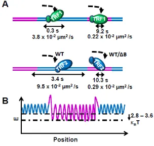
Brewer et al. 2012). The estimated radius of free TRF2 is estimated as 10 nanometers based on crystal structure of the Myb type and dimerization domains (Fairall, Chapman et al. 2001, Court, Chapman et al. 2005). The expected upper limit for diffusion constants for a single red QD labeled TRF2 sliding on DNA without curvilinear motion is 17.8 µm2/s. This is 187-468 fold higher than the measured diffusion constants for TRF proteins (between 3.8e-2 and 9.5e-2 µm2/s). This calculation supports the notion that TRF proteins slide on DNA while rotating, following along the DNA phosphate backbone.
Assuming protein rotation around the DNA helix, the expected upper limits for diffusion constants are based on a modified version of the Stokes-Einstein relation
𝑫𝟏,𝒄𝒂𝒍 = 𝑲𝑩𝑻 𝟔𝝅𝜼𝒂[𝟏 + (𝟒𝟖) ∙ (𝟐𝝅)𝟐∙ ( 𝒂 𝟑. 𝟒 ∙ 𝟏𝟎−𝟗) 𝟐 ] (34)
where η is the viscosity of the medium, α the radius of the particle, KB is Boltzmann’s constant, and T is the temperature.
The expected upper limits for diffusion constants and stepping rates for TRF2 proteins (with one red QD) with rotation-coupled diffusion are 0.021 µm2/s and 365492 steps/s, respectively. These numbers correspond to a diffusion rate of 0.42 µm2/s and a stepping rate of 7315292 steps/s without QDs.
The stepping rate is calculated by assuming the diffusion constant to occur as a series of steps of a single base pair using the following relationship
𝒌 = 𝒔𝒕𝒆𝒑𝒔
𝒔𝒆𝒄 (𝒏) = 𝟐𝑫 𝒍𝒃𝒑𝟐
where k is the stepping rate, D is the diffusion constant, and lbp is the length of one ds DNA
base pair (Hughes 1995).
3.5 Prediction of additional energy barriers
Furthermore, reduced diffusion constants relative to predicted values for unbiased 1-D diffusion indicates diffusion barriers present along the 1-DNA. These barriers can include DNA target sequences, obstructions, or alternative DNA structures (G quadruplex, nicks, gaps, legions). It is possible to calculate the energy barriers to protein stepping based on the difference between the observed and predicted stepping rates and by applying the Arrhenius equation (Hughes 1995).
𝒌 = 𝐞𝐱𝐩 (− 𝑬𝑨 𝑲𝑩𝒕)
(36)
𝐸𝐴 = −ln (𝑘) ∙ 𝐾𝐵𝑡 (37)
Then the additional energy barrier between two different regions of DNA can be calculated as follows: (Kad, Wang et al. 2010)
𝑬𝑨𝟏− 𝑬𝑨𝟐 = −𝐥𝐧 (
𝒌𝟏
𝒌𝟐) ∙ 𝑲𝑩𝒕
(38)
The relative free binding energy between the two regions can be defined as follows:
∆𝑮𝒃𝒊𝒏𝒅 = 𝑲𝑩𝑻 ∙ 𝒍𝒏(𝒌𝟏 𝒌𝟐)
(39)
where k1 and k2 are the equilibrium association constants for the two respective DNA
∆𝑮𝒃𝒊𝒏𝒅= 𝑲𝑩𝑻 ∙ 𝒍𝒏(
𝝉𝟏
𝝉𝟐)
(40)
CHAPTER 4: Cohesin SA2 is a sequence independent DNA binding protein but recognizes DNA ends and gaps
4.1 Cohesin background
The cohesin complex plays a role in a plethora of genome maintenance pathways. In eukaryotes the cohesin complex is integral for the proper segregation and alignment of sister chromatid (Michaelis, Ciosk et al. 1997, Remeseiro, Cuadrado et al. 2013). Improper
segregation of chromosomes can quickly lead to aneuploidy or genetic diseases (Kim, Kim et al. 2012, Taylor, Platt et al. 2014). Cornelia de Lange syndrome is caused by cohesin
disruption, and results in altered transcriptional regulation while maintaining standard chromatid separation, indicating that mutations or defects of Cohesin elements affect a variety of processes independent of DNA cohesion (Peters, Tedeschi et al. 2008).
The core cohesin complex consists of a tripartite ring structure with two arm proteins Structural Maintenance of Chromosomes 1 and 3 (Smc1 and Smc3) and a bridge protein Rad21in addition to Stromal Antibody 1 or 2 (SA1 or SA2) in vertebrates. This ring architecture makes Cohesin an ideal candidate for maintaining cohesion between sister chromatid separation during mitosis, or regulating transcription by establishing and
requirement for proper chromosome segregation, they do not play a role in the loading or unloading of the cohesin complex (Hou and Zou 2005, Rankin, Ayad et al. 2005).
Crystallography, electron microscopy, and biochemical assay based studies indicate that cohesin binds to the DNA by a topologic embrace (Haering, Lowe et al. 2002, Gruber, Haering et al. 2003, Murayama and Uhlmann 2014). How cohesin binds to chromatin to establish cohesion remains a controversial topic (Schmidt, Brookes et al. 2009).
4.2 Summary
Our paper on the DNA binding properties of cohesin protein SA2 is currently in submission. The paper in its current form is available in the appendix. Below there will be a brief summary of the paper.
the same DNA substrates indicated that SA2 had no change in diffusive behavior in the presence of telomere, centromere, or genomic DNA sequences.
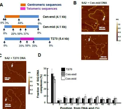
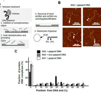
Curiously, our AFM results saw that SA2 showed a strong affinity for ends of DNA regardless of the sequence, length, or presence of overhang (Figure 3: SA2 does not show binding preference for telomeric or contromeric DNA sequences, but recognizes DNA ends.). Given the alternative roles of cohesin outside of cohesion, we postulated that SA2 had an affinity for regions of DNA damage. We tested the binding of SA2 to new DNA substrates that contained either nicks or gaps using AFM. SA2 had no binding affinity towards a single nick site, however severely nicked DNA did decrease the overall end binding of the SA2 protein. Introduction of a single stranded region of DNA 37 base pairs long significantly shifted the binding affinity of SA2. SA2 showed a significant affinity for the gapped region of the gapped DNA in addition to strong end binding (Figure 4: SA2 specifically binds to ssDNA gaps.). Fluorescence studies conducted with the ligated gapped DNA substrate revealed periodic binding along the DNA tightrope at intervals corresponding to the DNA length. SA2 binding to the gapped substrate was overwhelmingly static. There was a significant difference in the diffusion constant and alpha factor for SA2 on the gapped substrate as compared to all other DNA substrates (Figure 5: SA2 switches between searching and recognition modes on DNA tightropes containing ssDNA gaps.).
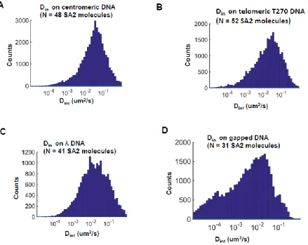
higher predilection for extremely low values (Dint < 10-4 µm2/sec), corresponding to regions where the SA2 encountered gap regions of DNA (Figure 6: Comparison of the distribution of interval based diffusion constants (Dint) for SA2 on different DNA tightropes.). Unlike SA1 on telomere DNA tightropes, SA2 showed no additional diffusive modes in the presence of gapped DNA. Our work has shown that SA2 is successfully able to bind to ds and ss DNA independent of other proteins or cofactors and shows a high affinity for DNA ends and gaps. Thus SA2 could act as a structural anchor for the cohesin complex to successfully bind to the DNA.
Figure 3: SA2 does not show binding preference for telomeric or contromeric DNA sequences, but recognizes DNA ends.
Figure 4: SA2 specifically binds to ssDNA gaps.
Figure 5: SA2 switches between searching and recognition modes on DNA tightropes containing ssDNA gaps.
Figure 6: Comparison of the distribution of interval based diffusion constants (Dint) for SA2 on different DNA tightropes.
CHAPTER 5: Functional interplay between SA1 and TRF1 in telomeric DNA binding and DNA-DNA pairing
5.1 Background
Proper chromosome alignment and segregation during mitosis depends on cohesion between sister chromatids. In vertebrates, the core cohesin complex consists of a tripartite ring assembled by Smc1, Smc3, Rad21, and either SA1 or SA2 (Remeseiro and Losada 2013). The cohesin complex is distributed along centromere and telomere regions of
chromosome arms (Wendt, Yoshida et al. 2008). Telomeres are nucleoprotein structures that prevent the degradation or fusion of linear chromosome ends by preventing them from activating the DNA damage response and double-strand DNA break repair mechanisms (Blackburn 2005, Palm and de Lange 2008, Holohan, Wright et al. 2014, Lin, Kaur et al. 2014). Surprisingly, cohesin rings do not play a major role in sister telomere cohesion. This role is replaced by SA1 and telomere binding proteins TRF1 and TIN2, however the DNA binding mechanism of SA1 and the unique telomere cohesion mechanism are poorly
5.2 Summary
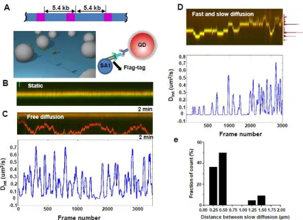
Recently we demonstrated that the N-terminal domain of SA1 (1-72 AA, SA1-N) binds to a DNA substrate containing telomere sequences (Bisht, Daniloski et al. 2013). To understand the SA1 DNA binding mechanism, we obtained full-length His- and Flag-tagged SA1 proteins. We carried out binding of SA1 on a telomeric DNA substrate containing 270 TTAGGG repeats (T270, 5.4 kb) and a control substrate (3.8 kb) containing only the non-telomeric (genomic) DNA sequences from T270. AFM imaging indicated that a higher percentage (41.9%) of SA1 bound at the telomeric region on the T270 DNA substrate compared to the same locations along the genomic DNA substrate (27.0%).
with the boundaries of the telomeric region (1.6 kb) and the spacing between two adjacent telomeric regions on T270 (5.4 kb).
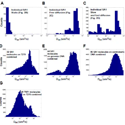
To further compare the dwell times of slow diffusion events displayed by mobile SA1 on different DNA substrates, I developed the ‘sliding window’ (40 frame, 2s) MSD analysis method to calculate a time interval-based diffusion constant (Dint, bottom panels in Fig. 1C and 1D). Distinct from static (< 0.5 X 10⁻³ µm2/sec, Figure 7: Full length SA1 alternates between fast and slow 1-D diffusion on T270 DNA tightropes.A) and fast free diffusion modes (> 10-1 µm2/sec, Figure 7: Full length SA1 alternates between fast and slow 1-D diffusion on T270 DNA tightropes.B), this analysis indicated that mobile SA1 molecules with fast and slow diffusion on T270 show a distinct peak at ~10-3 µm2/sec (Figure 7: Full length SA1 alternates between fast and slow 1-D diffusion on T270 DNA tightropes.C). Therefore, for calculating dwell times on DNA tightropes we used Dint value of 5.0 X 10⁻³ µm2/sec as the threshold to identify slow diffusion events. This Dint based analysis showed that the dwell times of individual SA1 slow diffusion events on T270 (1.17 s) are
genomic (0.14 ± 0.03 µm2/sec) or centromeric (0.11 ± 0.02 µm2/sec) DNA sequences. Additionally the alpha factor for SA1 on T270 was significantly smaller than on genomic DNA, which suggests protein pausing amid free diffusion at telomere sequences.
SA1 contains a unique AT-hook motif at its N-terminal domain which is not present on SA2 (Bisht, Daniloski et al. 2013). To determine whether or not SA1 slow diffusion events depend on its unique N-terminal domain, we purified SUMO-tagged SA1 N-terminal fragment (SA1-N). Analysis of the binding position of SA1-N from AFM images revealed that SA1-N binds specifically to telomere regions. Consistent with results from AFM imaging, incubation of SA1-N-QDs with T270 DNA tightropes resulted in substantial DNA binding. A significantly higher percentage of SA1-N molecules (74.3%) showed slow diffusion events (dwell time > 2.2 s) on T270 DNA than on genomic DNA (38.6%).
SA1 interacts directly with TRF1 through its N-terminal domain (Canudas,
Houghtaling et al. 2007). To evaluate how TRF1 affects the dynamics of SA1 on DNA, we directly images their interactions. Flag-SA1 and His-TRF1 proteins were orthogonally conjugated with red Ab-QDs and green SAv-QDs via antibody sandwich and BTtris-NTA linkage strategies respectively. A higher population of dual-colored SA1-TRF1-QD complexes (~60%) were static than single-colored SA1-QD alone (~35%) on T270 DNA tightropes. SA1-TRF1 complexes exhibited significantly reduced diffusion ranges compared to SA1 alone. Furthermore, the distance between dual-color QD-labeled SA1-TRF1
Consistent with previous results, we observed that TRF1 molecules formed protein tracts that mediate DNA-DNA pairing on T270 DNA (Griffith, Bianchi et al. 1998). In the presence of both TRF1 and SA1 the average SA1-TRF1 mediated DNA-DNA pairing tract length increased significantly. The location of SA1 on TRF1-mediated DNA-DNA pairing tracts was random.
Figure 7: Full length SA1 alternates between fast and slow 1-D diffusion on T270 DNA tightropes.
(A) Ligated T270 DNA substrate (top panel) and the DNA tightrope assay setup (bottom left panel). (B-D) Dynamics of full length Flag-SA1 on T270 DNA tightropes. Kymographs of SA1 molecules being static (B), showing free 1-D diffusion (C), and alternating between fast and slow 1-D diffusion (D) on T270 DNA. Scale bars (y-axis): 1 µm. Equimolar
Figure 8: Comparison of the distributions of interval based diffusion constants (Dint) for SA1 TRF1.
(A-C) Distributions of Dint for individual SA1 molecules on T270 DNA tightropes with static (A, kymograph in Fig. 1B), free diffusion (B, kymograph in Fig. 1C), and alternation
CHAPTER 6: Telomere maintenance pathway
6.1 Introduction to telomeres
Telomeres play important roles in maintaining the stability of linear chromosomes (de Lange 2002, Cech 2004, Blackburn 2005, de Lange 2005, Sfeir 2012). The telomeric
structure allows a cell to distinguish between natural chromosome ends and double-stranded DNA breaks. As such, telomeres prevent the inappropriate activation of DNA damage signaling pathways, which can lead to cell cycle arrest, senescence, or apoptosis
(Smogorzewska and de Lange 2004). Loss of telomere function can activate DNA repair processes, leading to nucleolytic degradation of natural chromosome ends and end-to-end fusions. Telomere dysfunction and associated chromosomal abnormalities have been strongly associated with age-associated degenerative diseases and cancer (Wright and Shay 2000, Maser and DePinho 2002). Great progress has been made in the last 20 years in
understanding telomere biology in model systems, including ciliates, yeast, drosophila, plants, and mouse (Giraud-Panis, Pisano et al. 2010, Lewis and Wuttke 2012, Wellinger and Zakian 2012).
2013). A specialized protein complex, called shelterin or telosome, binds to and protects telomeres at chromosome ends (Verdun and Karlseder 2007). In humans, this complex consists of six core proteins: duplex TTA-GGG repeat binding factor-1 (TRF1) and -2 (TRF2), the single-stranded telomeric DNA binding protein protection of telomeres-1 (POT1), TRF1-interacting nuclear protein 2 (TIN2), POT1- and TIN2-organizing protein (TPP1), and transcriptional repressor/activator protein RAP1 (Cech 2004, Songyang and Liu 2006, Verdun and Karlseder 2007). The RPA-like CTC1-STN1-TEN1 complex binds to ssDNA and protects telomeres independently of the POT1 protein, and acts as a terminator of telomerase (Miyake, Nakamura et al. 2009, Chen, Redon et al. 2012). Shelterin proteins interact with numerous protein factors, including proteins involved in DNA recombination and repair, such as ERCC1-XPF, WRN, BLM, and DNA-PK (Zhu, Niedernhofer et al. 2003, Opresko, Otterlei et al. 2004, Verdun and Karlseder 2007, Bombarde, Boby et al. 2010). Adding to the complexity of telomere structures, telomeric repeat-containing RNA (TERRA) was identified as an integral part of telomeric heterochromatin (Luke and Lingner 2009, Feuerhahn, Iglesias et al. 2010). TERRA is associated with TRF2 and a large number of RNA-binding proteins, and is implicated in telomere structural maintenance and
heterochromatin formation (Deng, Norseen et al. 2009, Lopez de Silanes, Stagno d'Alcontres et al. 2010).
Telomeres can adopt different types of open or closed (capped) conformation.
Comeau et al. 1999, Murti and Prescott 1999, Munoz-Jordan, Cross et al. 2001, Cesare, Quinney et al. 2003, Luke-Glaser, Poschke et al. 2012). Telomeres can be maintained by the recombination-dependent alternative lengthening of telomeres (ALT) pathway in telomerase-negative tumors. The ALT pathway is accompanied by the generation of duplex or single-stranded DNA circles formed from telomeric repeat sequences (t-circles) (Tomaska, Nosek et al. 2009). G-rich sequences have been shown to form discrete four-stranded structures termed quadruplexes in vitro (Fry 2007). Studies using an engineered, structure-specific
G-quadruplex antibody provided evidence that G-G-quadruplex DNA exists in telomeres in vivo (Maizels 2006, Biffi, Tannahill et al. 2013, Lam, Beraldi et al. 2013). Stable G-quadruplex DNA plays important roles in the regulation of telomere extension and organization, as well as pairing of homologous chromosomes (Fry 2007).
Karlseder, Broccoli et al. 1999). Overexpression of TRF2 in telomerase-negative cells prevents short telomeres from fusing and delays the onset senescence (van Steensel, Smogorzewska et al. 1998). Furthermore, TRF2 plays important roles in the assembly of telomeric chromatin (Benetti, Schoeftner et al. 2008). Importantly, post-translational modification of TRF1 and TRF2 regulate their functions, including DNA binding,
dimerization, localization, degradation, and interactions with other proteins (Walker and Zhu 2012). In addition, several groups have reported DNA binding and gene regulation functions for both TRF1 and TRF2 proteins outside of telomeres (Bradshaw, Stavropoulos et al. 2005, Fouche, Cesare et al. 2006, Mao, Seluanov et al. 2007, Zhang, Pazin et al. 2008, Simonet, Zaragosi et al. 2011, Yang, Xiong et al. 2011, Bosco and de Lange 2012).
Both TRF1 and TRF2 contain a TRFH domain that mediates homodimerization and a C-terminal Myb type domain that mediates sequence-specific binding to telomeric DNA (Court, Chapman et al. 2005). In both proteins, the DNA binding domain and the
dimerization domain are joined together by long linkers (~100 amino acids in TRF1 and 150 amino acids in TRF2). The dimerization domains from human TRF1 and TRF2 have the same α-helical architecture (Fairall, Chapman et al. 2001). However, TRF1 and TRF2 dimerization interfaces feature unique interactions that prevent heterodimerization. Solution structures of Myb domains of TRF1 and TRF2 bound to DNA with the sequence
DNA binding activity than that of TRF1 (equilibrium constants Kd 750 nM vs 200 nM respectively). A single amino acid change (lysine on TRF2 to arginine on TRF1) is the main contributor to this difference in binding affinity.
simultaneously bind to TERRA and telomeric G-quadruplex DNA (Biffi, Tannahill et al. 2012), and a TERRA-like RNA molecule greatly reduces its ability to condense DNA (Poulet, Pisano et al. 2012).
TRF1 and TRF2 are the only shelterin proteins that bind to duplex telomeric DNA with high affinity. Dynamic movements on DNA, such as 1-demensional (1-D) sliding (translocating while maintaining continuous DNA contact), jumping and hopping (microscopic dissociation and rebinding events), are essential for a protein to achieve its function inside cells where nonspecific DNA is in vast excess and bound by histones and other proteins (Berg, Winter et al. 1981, von Hippel and Berg 1989, Gorman and Greene 2008, Tafvizi, Mirny et al. 2011). How TRF1 and TRF2 find their cognate sites and protein partners to form the shelterin complex, and regulate the functions of proteins involved in DNA repair and cell-cycle progression are not fully understood (de Lange 2010).
6.2 Summary
Here we used single-molecules fluorescence imaging to study the dynamics of quantum dot (QD) labeled TRF1 and TRF2 proteins on λ DNA and DNA substrates
containing alternating telomeric and non-telomeric sequences. To determine whether TRF1 and TRF2 slide or hop, we evaluated the effect of ionic conditions on the dynamic
should not affect the diffusion constants of a sliding process, but should elevate the diffusion constants of hopping (Berg, Winter et al. 1981, Komazin-Meredith, Mirchev et al. 2008, Gorman, Fazio et al. 2010). While TRF1 followed a trend of decreasing diffusion constants as the ionic strength increased, TRF2 was highly motile on λ DNA across all ionic strengths and showed no change in diffusion constant. TRF1 also showed a slight increase in the α factor proportional to the ionic strength, while TRF2 did not show any significant variation with ionic strength, suggesting an unbiased random walk. Additionally, both TRF1 and TRF2 bound to the ligated T270 DNA tightropes with regular spacing. For both TRF1 and TRF2, the distribution of the distances between nearest-neighbor binding fit well to the sum of two Gaussian distribution functions centered at ~1.6 and 3.2 µm (consistent with the expected spacing of the telomeric regions).
We also examined how far single molecules of TRF1 and TRF2 could slide on the ligated non-telomeric DNA versus ligated T270 DNA. TRF1 and TRF2 displayed distinct diffusion ranges on telomeric DNA, but not on non-telomeric DNA. The diffusion range was invariant across all time windows (~10-100 s), ruling out the possibility that the short range diffusion observed was due to shorter video lengths. Instead, this finding suggests that once the molecules are within a telomeric region, they tend to remain there. We explored the possibility that short range diffusion was caused by multiple proteins binding to the same telomeric region and restricting 1-D sliding. However at lower TRF2 concentration, the short diffusion range did not change. We noted that in many cases TRF proteins binding to
sequences. To ensure that this confinement would not artificially reduce the apparent
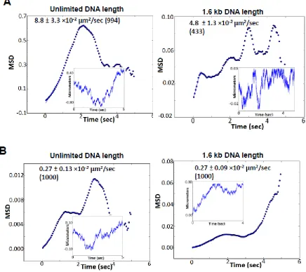
diffusion constant, I designed a 1-D diffusion of proteins on a linear DNA lattice of unlimited length versus a 1.6 kb total length, which mimics the (TTAGGG)270 region. These
simulations revealed that confinement within 1.6 kb DNA does not significantly reduce the observed diffusion constant at the (TTAGGG)270 region (Figure 10: Computer simulations of diffusion by modeling random walk of proteins on a 1-D DNA lattice using PythonTM
programming language.). In addition, camera based time-averaging was not a major contributor to the observed slower diffusion constants at the telomeric region under these experimental conditions.