SRIDHARAN, SAVITHA. Fair Queueing Algorithms for QoS Support in Packet Switched Networks. (Under the direction of Dr. Yannis Viniotis, in association with Agere Systems.)
The rapid growth of telecommunications has led to a demand for convergence of voice, video and data integration over traditional data networks. This has strained the current packet-switched networks which are not very well-suited for voice and video applications. Quality-of-service-aware, high-speed packet switches are being designed to alleviate the problems in traditional networks. The key motivation of this thesis was to analyze scheduling algorithms in order to guarantee Quality of Service for high-speed packet networks, particularly for voice applications.
Biography
Acknowledgement
I sincerely thank my advisor, Dr.Yannis Viniotis for his invaluable guidance and sup-port through my graduate studies. I would like to sincerely thank him for encouraging me in pursuing my interests in the area of Network Processor Architecture with Agere Systems for my thesis. I thank him for his constant support and encouragement.
I am equally thankful to Curtis Lee Hillier and Mark Emery, my supervisors at Agere Systems, Austin, during my internship in Summer 2005 for all their encourage-ment and for offering me an opportunity to work at Agere Systems for my thesis. I would like to sincerely thank Paulus Sastrodjojo, David Sonnier, Rob Munoz and Bal-akrishnan Sundararaman for all the support and instant answers to all the questions I had during my research at Agere.
I am very grateful to Dr. Devetsikiotis and Dr. Byrd for agreeing to be on my thesis committee and for the valuable feedback regarding the thesis document.
I am greatly indebted to my parents and my brother for everything they have done for me. Without their love and support, I would never have been able to succeed in my endeavors. My sincere thanks to Bhaskar for helping me and providing me help through my graduate school here.
Contents
List of Tables vii
List of Figures viii
1 Introduction 1
1.1 Motivation . . . 1
1.2 Outline of Thesis . . . 2
2 Fair Packet Scheduling 3 2.1 Introduction . . . 3
2.1.1 Packet Scheduling Algorithms . . . 5
2.1.2 Packet Switch Architectures . . . 5
2.2 Scheduling Output Buffers . . . 8
2.2.1 Classifying Schedulers . . . 8
2.2.2 Shapers and Schedulers . . . 10
2.3 Requirements of a Packet Scheduler . . . 12
2.4 Complexity of a Scheduling Algorithm . . . 14
2.4.1 Design Complexity . . . 14
2.4.2 Implementation Complexity . . . 16
2.5 Applications of a Fair Packet Scheduler . . . 16
3 Understanding QOS in Packet Switched Networks 18 3.1 Classifying Packet Networks . . . 18
3.1.1 Classification by Packet Size . . . 18
3.1.2 Classification by Packet Route . . . 20
3.2 Traffic Types in Packet Networks . . . 21
3.3 Achieving QoS . . . 22
3.4 Metrics for QOS Guarantee . . . 26
3.4.1 Bandwidth Sharing . . . 27
3.4.2 Packet Delay . . . 28
3.4.3 Delay Jitter . . . 29
3.5 Fairness Index . . . 33
3.5.1 Jain’s Fairness Index . . . 34
4 Packet Scheduling Algorithms 36 4.1 Background Work . . . 36
4.1.1 Generalized Processor Sharing (GPS) . . . 36
4.2 Weighted Jitter Deadline Scheduling . . . 38
4.2.1 Category 1 : Simple WJ-EDF . . . 39
4.2.2 Category 2: Shaped WJ-EDF . . . 41
5 Simulation Study 44 5.1 Architecture Overview . . . 44
5.2 Simulation Environment . . . 47
5.2.1 Setup 1: Behavioral C model . . . 48
5.2.2 Setup 2: Agere’s SDE . . . 50
5.3 Metrics and Simulation Variables . . . 52
5.4 Observations and Performance Analysis . . . 54
5.4.1 Fairness Index Analysis . . . 55
5.4.2 Jitter Analysis . . . 60
5.5 Weighted-Jitter EDF . . . 65
6 Conclusion and Future Work 69 6.1 Findings and Conclusion . . . 69
6.2 Future Plans . . . 70
Bibliography 71
List of Tables
2.1 Comparison of Work Conserving and Non Work Conserving Schedulers 9
2.2 Comparison of sorted and frame-based schedulers . . . 10
5.1 T for different arrival rates and packet sizes (IETF). . . 61
5.2 davg for different arrival rates and packet sizes (ITU-T). . . 61
A.1 Single Traffic Flow fed to OC-3 Scheduler (Sample Size n=10) . . . . 77
A.2 Two Traffic Flows fed to OC-3 Scheduler (Sample Size n=10) . . . . 78
A.3 Four Traffic Flows fed to OC-3 Scheduler (Sample Size n=10) . . . . 79
A.4 Comparison of Scheduling Algorithms for traffic flow feeding the OC-3 Scheduler (Sample Size n=10) . . . 79
A.5 Comparison of Scheduling Algorithms for two traffic flows feeding the OC-3 Scheduler (Sample Size n=10) . . . 80
A.6 Comparison of Scheduling Algorithms for two traffic flows feeding the OC-3 Scheduler (Sample Size n=10) . . . 80
A.7 Comparison of Scheduling Algorithms for four traffic flows feeding the OC-3 Scheduler (Sample Size n=10) . . . 81
A.8 Deadlines applied to packets of different sizes . . . 82
A.9 Deadlines applied to packets arriving at different input rates . . . 83
A.10 Algorithm Legend . . . 83
A.11 1-Point CDV for Single Input Flow . . . 84
A.12 2-Point PDV for Single Input Flow . . . 84
A.13 Average 1-Point CDV for Four Input Flows . . . 85
List of Figures
2.1 Basic Architectural Components of a Packet Switch . . . 6
2.2 Kleinrock’s Delay Conservation law for work-conserving schedulers. . 8
2.3 Packet Processing Elements in a network device. . . 11
2.4 An example of a Hierarchical Scheduler . . . 12
3.1 Example of bandwidth sharing. . . 27
3.2 Understanding Delay and Delay Jitter. . . 31
3.3 Loss graph . . . 32
4.1 Simple WJ-EDF scheduler . . . 39
4.2 Shaped WJ-EDF scheduler structure. . . 42
5.1 APP650 Architecture: Block Diagram. . . 45
5.2 Sched-650 Architecture: Block Diagram. . . 46
5.3 Behavioral C Model: Block Diagram . . . 48
5.4 Testcase Data File format. . . 48
5.5 Result File: Jitter Measurements. . . 50
5.6 Agere SDE’s Java-based GUI. . . 50
5.7 Behavior of packets from two traffic flows at the output of Sched-650. 55 5.8 Single flow: Output rate of a scheduler operating at OC-3 for various input rates. . . 56
5.9 Two traffic flows: Output rate of a scheduler operating at OC-3, for various input rates. . . 57
5.10 Four traffic flows: Output rate of a scheduler operating at OC-3, for various input rates. . . 58
5.11 Two input traffic flows: Comparison of scheduling algorithms. . . 59
5.12 Four input traffic flows: Comparison of scheduling algorithms. . . 60
5.13 Comparison of 1-Point CDV with number of flows for Packet Size = 1 Cell . . . 62
5.15 Comparison of 1-Point CDV with number of flows for Packet Size = 2
Cells . . . 63
5.16 Comparison of 2-Point PDV with number of flows for Packet Size = 2 Cells . . . 63
5.17 Comparison of 1-Point CDV with number of flows for Packet Size = 3 Cells . . . 64
5.18 Comparison of 2-Point PDV with number of flows for Packet Size = 3 Cells . . . 64
5.19 Comparison of 1-Point CDV with number of flows for for Packet Size = 8 Cells . . . 65
5.20 Comparison of 2-Point PDV with number of flows for Packet Size = 8 Cells. . . 65
5.21 Comparison of 1-Point CDV with packet size for Single Flow. . . 66
5.22 Comparison of 2-Point PDV with packet size for Single Flow. . . 66
5.23 Comparison of 1-Point CDV with packet size for four Flows. . . 67
5.24 Comparison of 2-Point PDV with packet size for four Flows. . . 67
5.25 Deadlines to packet departures under EDF and WJ-EDF for different packet sizes. . . 68
Chapter 1
Introduction
1.1
Motivation
Recent trends in telecommunication, computing and entertainment along with faster networks have led to a demand for technology convergence. The idea of inte-grating voice, data and video over a single network, which is easily accessible for a large number of users is gaining popularity. These integrated networks help simplify consumer needs as well as reduce maintenance and support costs for their operator companies. Traditional circuit-switched networks are not suitable for these applica-tions and have led to the development of Packet Switched Networks or PSN.
Telephone systems and virtually all data communication networks mostly used circuit-switched networks during the late 1960s. Circuit-switched networkspreallocate transmission bandwidth for an entire call or session, hence guaranteeing capacity for the user. Though dedicating resources to facilitate a single call ensures quality of service (QoS), it is a costly proposition, because the resources are not utilized completely during the duration of the call or session. In the beginning of the 1970s, a competing approach of dynamic allocation of bandwidth was introduced in building communication networks, now popularly called as packet switched networks.
trans-mitted through network nodes until they reach the destination, taking (hopefully) the most expedient route. The receiver uses the destination address in the packet to identify its blocks and reassemble the blocks into the original information. Thus PSNs are able to share network resources, and provide a cost-effective, flexible and reliable technology. However, it is not always possible to guarantee bandwidth in a packet switched network. Due to the stochastic nature of packet queuing in network nodes, delay varies from packet to packet based on the network traffic load. Even under lightly-loaded network conditions, delays are typically larger than in the circuit switched networks.
Packet switched networks are good candidates for a converged network. Trans-mitting voice and constant bit-rate (CBR) traffic on a packet-switched network is challenging because of the long transmission delay and delay variations associated with these networks. In order to alleviate these problems, Quality of Service-aware, high-speed packet switched networks are being designed to reduce end-to-end trans-mission delays. Analysis and design of scheduling algorithms to guarantee QoS in high-speed packet networks is the key motivation of this thesis.
1.2
Outline of Thesis
Chapter 2
Fair Packet Scheduling
2.1
Introduction
Packet Switching is a method in which data is divided into units called packets before being transmitted to the destination. The packets can arrive at the destination through completely different routes. The networks which use this method to transfer data are known as Packet Switched Networks [1]. The other kind of networks are circuit-switched networks, where a physical connection is present between the source and destination when transmitting data.
Packet Switched Networks has proved to be good candidates for network conver-gence, that is integrating voice, video and data applications. This is because as long as the packets adhere to the network protocol the underlying data can be of different types. Many different kinds of networks inter-operate to support many different kinds of services ranging from real-time voice and video applications like voice-over-IP and videoconferencing, streaming video, interactive applications like web browsing and gaming, and background applications like remote access applications, file transfer and e-mail.
be aware of their peak bandwidth utilization during the connection setup phase. A new flow requesting connection may be admitted into the network until the sum of the maximum bandwidth requirements of the already connected flow is less than the link capacity under consideration. Consider a node in a network that can support a total bandwidth, Ctotal. Let us consider the case of a new flowk requesting this node
a bandwidth of Ck at an instant when the node is already supportingn connections,
each utilizing C1, C2,..., Cn. Flow k will be allowed to share the resources of this
node only if,
Ck ≤Ctotal− n
j=1
Cj (2.1)
Dedicating resources to facilitate a selected number of users is a costly proposi-tion, because the resources are not utilized completely during the duration of the connection. In the case of a packet switched network, a technique called dynamic allocation of resources for flows is used. The common dynamic resource allocation approaches include statistical multiplexing and packet scheduling algorithms. Statis-tical multiplexing is one of the most common techniques in network system design primarily because of simplicity of design and implementation.
2.1.1
Packet Scheduling Algorithms
One of the mechanisms employed to control the resources allocated to packets from different connections by deciding which packet is to be transmitted next on the output link is called apacket scheduling algorithm. A packet scheduler forms a small but a very critical part of network system design. The efficiency and fairness (Refer to section 3.4) achieved by a scheduling algorithm is dependent on a number of factors such as number of queues that are serviced by the algorithm, bandwidth required by each flow, arrival pattern of traffic in each of the flows, length of the queues to hold these flows and size of packets arriving into the queues.
Packet scheduling algorithms may be implemented in hardware or in software. The scheduling algorithm must also take into consideration the kind of traffic that it must handle, ranging from small fixed-size packets like ATM cells carrying real-time voice to large variable-size packets like Jumbo Ethernet frames carrying best-effort data. Therefore, the scheduling algorithms must be designed in such a way that they can satisfy both the strict performance needs of real-time applications like voice and video, as well as the fair network resource sharing needed for best-effort traffic. Meeting these multiple restrictions makes design of a scheduling algorithm a challenging task. These algorithms are further constrained by the underlying packet switch architectures and buffering mechanisms.
2.1.2
Packet Switch Architectures
Packet switches are designed to serve two main functions:
1. Routing: When a packet arrives at the input port, the packet switch must take a decision about its next hop towards its destination. Once the decision is made, the packet is routed to the appropriate output port.
of their applications. The performance criteria may vary from application to application, ranging from the highest possible utilization of the expensive re-sources, the lowest possible latency, fair allocation of resources to competing users (QoS guarantees) or combinations of these.
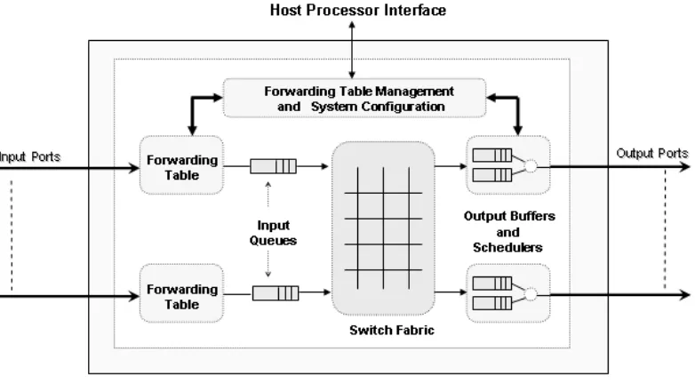
The basic architectural components of a packet switch, keeping these functions in mind, have been captured in Figure 2.1.
Figure 2.1: Basic Architectural Components of a Packet Switch
1. Forwarding Engine and Policer: The implementation of this component in switches depends on the function of the switch. The forwarding engine is also commonly referred to as the classifier. For example, let us consider a Ethernet Layer 2 Switch. When a packet arrives, its destination MAC address is looked up in a forwarding table. If the address is found, the packet is sent to an appropriate output port after updating its next-hop MAC address. The switch can also be programmed to discard corrupted or non-conforming packets.
traffic rate exceeds the configured maximum output rate (peak). In most cases, the policing block does not contain buffers and hence avoids delays due to queuing. However, bursty traffic is propagated through this block, and hence does not help in smoothening the traffic flow.
2. Input buffers: This may be a single FIFO or multiple FIFOs per input port in an input-buffered switch. Multiple FIFOs are used to eliminate head-of-line blocking, discussed a little later in this section. A scheduler may be needed to arbitrate packets from multiple queues [3].
3. Switch Fabric: This is also commonly referred to as backplane. The common fabric types include shared memory, bus, crossbar, ring structure and multistage networks. The packets may be buffered while the packet waits its turn to be transferred across the backplane.
4. Output buffers and scheduler: Packets may be buffered as they wait for their turn to be transmitted out of the output port. Schedulers can have sim-ple algorithms like First-Come, First-Serve or more comsim-plex algorithms like Weighted Round Robin or Weighted Fair Queuing in order to distinguish dif-ferent priority classes and meet QoS guarantees. This will be covered in greater detail in Section 2.1.
2.2
Scheduling Output Buffers
2.2.1
Classifying Schedulers
Networking designers and engineers have invented and studied a myriad of packet scheduling algorithms for years, but the design of an ideal scheduler (exhibiting per-formance of GPS or close to it) is still an extremely challenging problem. These multitudes of packet scheduling algorithms, varying in their ease of implementation and performance, can be characterized into the following categories:
1. Work-Conserving or Non Work-Conserving scheduler : A scheduler is consid-ered work-conserving if it never leaves the shared output link idle when there is a packet buffered in the system. First-come First-serve (FCFS), Round Robin (RR), Weighted Round Robin (WRR) and Weighted Fair Queuing (WFQ) schedulers are work-conserving in nature.
Kleinrock’s Delay Conservation law for work-conserving schedulers states that one flow cannot be given preferential treatment (i.e., reduced delay) without hurting the others. Consider N flows arriving at a scheduler as shown in Fig-ure 2.2.
Figure 2.2: Kleinrock’s Delay Conservation law for work-conserving schedulers.
According to the law,
N
i=1
whereλi is the average utilization of flowi,di is the average delay of flowi due
to the scheduler, C is a constant independent of the scheduling policy, λtotal is
the total utilization and dF IF O is the average delay of a single first-in first-out
queue with no particular scheduling.
Further,
λn =rnμn (2.3)
wherern is the mean packet rate in packets/sec and μn is the mean per-packet
service rate in seconds/packet. This concludes that some flows can receive lower delay only at the expense of longer delay from other flows.
On the other hand, a non-work conserving scheduler may remain idle, even when there are packets buffered in the system. Each packet buffered in the system is associated with an eligibility time and the scheduler transmits the packet from the system when the packet is eligible. This kind of scheduler can alternatively be called a regulator and helps in “smoothing” of packet flows. The output flow is controlled and makes downstream traffic more predictable.
Table 2.1: Comparison of Work Conserving and Non Work Conserving Schedulers Work Conserving Non Work Conserving
Link utilization Good Under-utilized
End-to-end delay Low High
Jitter High Less
Complexity Simple Not Efficient 1
2. Sorted Priority or Frame-based scheduler
that order. Start-time Fair Queuing (SFQ), Self-clocked Fair Queuing (SCFQ), Weighted Fair Queuing (WFQ) and Worst-case Fair Weighted Queuing (WF2Q) are examples of sorted-priority schedulers.
On the other hand, frame-based schedulers neither maintain any global variable nor do they require sorting among packets. Instead, time is divided into frames of fixed or variable length. In a fixed size frame, a frame is divided into slots for different sessions. Sessions reserve the maximum amount of traffic they are allowed to transmit during a frame period. As a result, the scheduler can remain idle if sessions transmit less traffic than their reservations over the duration of a frame. Hierarchical Round Robin and Stop-and-Go queuing are constant frame sized frame-based schedulers. In contrast are the variable frame sized frame based schedulers like Weighted and Deficit Round Robin, in which the scheduler visits all the non-empty queues in a round-robin order. A new frame can start early if the traffic from a session is less than its reservation. It can be clearly seen that the former frame-based schedulers are non work-conserving while the latter frame-based schedulers are work conserving in nature.
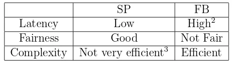
Table 2.2: Comparison of sorted and frame-based schedulers
SP FB
Latency Low High2
Fairness Good Not Fair
Complexity Not very efficient3 Efficient
2.2.2
Shapers and Schedulers
Traffic characteristics and requirements of various flows in networking applications vary widely. Architectural design of networking devices handling these traffic types needs to be well analyzed in order to support the spectrum of traffic demands. Packet 2A contending flow with a much higher reserved rate can lead to larger latency for lower reserved
rate flows.
3This is due to the complexity involved in computing the virtual time function, which purely
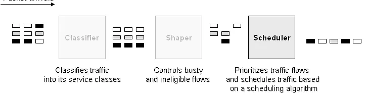
processing in network components like switches, routers or network processors is partitioned into a sequence of processing elements, each processing element having a specific role to play.
Figure 2.3: Packet Processing Elements in a network device.
Figure 2.3 highlights those processing elements in a network device which play a critical role in scheduling. In most cases, either a regulator or policer is used with a scheduler.
• Regulator:
In most cases, a non work-conserving scheduler for traffic shaping is imple-mented in this block. When the traffic rate exceeds the maximum output rate, the excess packets are delayed in the regulator by buffering in a queue. The shaping scheduler gradually transmits the eligible packets to the scheduler block over time, resulting in a smooth output rate. However, buffering of packets leads to introducing delay to the traffic flow. Regulation is usually done for outbound traffic.
• Scheduler:
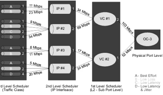
Sometimes schedulers are implemented hierarchically. Similar traffic types are first grouped and scheduled by a Level 1 scheduler. Varying traffic types from Level 1 are then buffered and scheduled again by a Level 2 scheduler. Figure 2.4 shows an example of a hierarchical scheduler [4].
Figure 2.4: An example of a Hierarchical Scheduler
[5] is an example that holds good for those applications which only support a select set of group rates. All sessions with the same group rate are grouped together at Level 1 and are then scheduled according to Smallest Eligible Finish Time policy (SEFF) at Level 2. This grouping architecture reduces the com-plexity of the scheduler from one that scales with the number of sessions to the one that scales with the number of distinct rate groups.
2.3
Requirements of a Packet Scheduler
The scheduling algorithm assigns different priorities to packets from different ap-plications (varying in service classes or rates of operation) and places these different priority packets in different queues. An arbitrator then makes the choice of the queue to serve in the order of their priority levels.
A packet scheduler must meet the following fundamental requirements:
A scheduling architecture must efficiently utilize the bandwidth, being able to handle bursty sources. For example, statistical multiplexing of flows can help in achieving efficient bandwidth resource allocation [6].
2. Isolation of Flows
An application flow must be isolated from the effects of other competing flows (which could be undesirable misbehaving sessions) by a fair scheduling algo-rithm. The algorithm must be able to meet the QoS guarantees of a flow when another flow sharing its output link is misbehaving. This characteristic of a scheduler can be applied in network security applications to defend against Dis-tributed Denial of Service (DDoS) attacks, discussed in Section 2.5.
3. End-to-End Delay Guarantees
End-to-end delay in a packet network is usually defined as the time taken for a packet to be transmitted across a network from source to destination. It is a function of the network design and scheduler architecture in its nodes. Maintaining a low end-to-end delay bound for any session is one of the key requirements of a packet scheduling algorithm. The algorithm must provide end-to-end delay guarantees for individual sessions. A work-conserving scheduler is used in most architectures to meet the delay guarantee.
4. Ease of Implementation
A scheduling algorithm must have a simple implementation with minimum time to make a scheduling decision. This forces a hardware implementation of a scheduler for high-speed networks. A software implementation may be consid-ered for packet networks operating at lower speed or handling larger packet size, but the key point to be kept in mind is the rate at which a scheduling decision is made must be kept close to the rate of arrival of the packets.
5. Scalability
good scheduling algorithm must perform well for large numbers of flows.
O-notation is a measure of scalability that characterizes the complexity of an algorithm with respect to execution time and implementation size. A scheduling algorithm of O(1) complexity is considered ideal.
6. Fairness
Fairness of a packet scheduling algorithm, in most cases, is defined in terms of bandwidth allocation among competing flows. A fair scheduler must be able to
• Provide bandwidth guarantees to backlogged flows in a short time span, independent of past usage of the output link bandwidth by the flows.
• Allocate the unused output link capacity to the competing flows in pro-portion to their “weights” (or reserved rates).
Requirements 1 to 5 are applicable to any scheduling algorithm while a packet scheduling scheme is considered fair if requirement 6 is met. These requirements will help define the metrics to characterize the performance of an algorithm and its suitability for QoS support in packet switched networks. The metrics are enumerated and analyzed in Section 3.4.
2.4
Complexity of a Scheduling Algorithm
In high-speed network environments, schedulers are usually implemented in hard-ware (network processor or routers) rather than in softhard-ware. The implementation complexity of a scheduling discipline must be taken into consideration, in addition to the algorithmic complexity.
2.4.1
Design Complexity
1. Time complexitybe to provide the highest degree of fairness in resource allocation and the least end-to-end delay keeping the time complexity of an algorithm low.
For example, consider any priority-based scheduling architecture with a maxi-mum of N flows that shares an output link. It involves the following steps:
• Priority Tag Computation: This may involve computing a virtual time function, a weight based priority value, etc.
• Insertion into a sorted priority list.
• Selection of highest priority flow or packet: The priority given to a flow depends on the scheduling algorithm used. For example, in Earliest Dead-line First scheduling discipDead-line, the highest priority value may be given to the packet with the earliest deadline.
In general, the worst-case algorithmic complexity for maintaining a sorted pri-ority queue with N arbitrary entries is O(log(N)). A (lower time-complexity) sorted priority queue can be realized in a high-speed network by either using an efficient data structure, an efficient algorithm or by exploiting the parallelism feasible in a hardware implementation.
2. Regulation before scheduling
Most implementations of aregulator-cum-scheduler architecture involve two sep-arate priority queue data structure solutions. Moving packets from regulator to scheduler may become a point of concern in high-speed implementations.
3. GPS-relative delay or Latency
complexity of any scheduling algorithm that guarantees O(1) GPS-relative de-lay bound is ω(log(N)), where ω(f(n)) is the loose lower boundary of function f(n).
2.4.2
Implementation Complexity
1. Memory Access CostAppropriately partitioning memory and access requirements between on-chip and off-chip memory can directly impact the performance of a network sys-tem design. On-chip memory is expensive but provides low latency and high bandwidth. On the other hand, off-chip memory is relatively inexpensive but increases the power consumption during the activity on off-chip buses and faces higher bandwidth and latency restrictions. Data dependencies between off-chip access and storage of priority tags in off-chip memory can degrade the perfor-mance of the algorithm.
Designing a scheme that exploits the parallelism of on-chip memories (pipelin-ing) with limited number of off-chip memory references can help in an cost-effective, high speed implementation.
2. Complexity of basic operations
It is advisable to reduce logic inhigh-speed hardware implementations and hence speed up the most basic operations like add, multiply, subtract, divide, compare, memory read and write. Computation of priority tags or virtual time1 functions involve these basic operations.
2.5
Applications of a Fair Packet Scheduler
Fair schedulers have found widespread implementation in network processors, switches and routers, residential and corporate networks. Some applications include:
Fairness in scheduling algorithms is essential to protect flows from other mis-behaving flows triggered by deliberate misuse or malfunctioning software on routers or end systems. Rate limiting traffic in packet schedulers can be used to defend against packet flooding and related DoS attacks that allow customers their share of utilization bandwidth even in the face of attacks.
2. Smoothing techniques in multimedia applications.
Chapter 3
Understanding QOS in Packet
Switched Networks
In the previous chapter, the study of output queue schedulers and its real-world applications was discussed in detail. This chapter starts by describing packet-switched networks and their categories, common service class categories and the need for QoS. Then, QoS metrics that can be used to estimate the performance of a scheduling al-gorithm in supporting multiple traffic types (commonly referred to asservice classes) are defined.
3.1
Classifying Packet Networks
Packet networks can be classified in various different ways, based on packet route, type of packet, size of packet, etc. Here we discuss two main ways of classifying packet networks, by packet size or by the way information flows from source to destination.
3.1.1
Classification by Packet Size
A very common example of fixed-size packet network is Asynchronous Transfer Mode (ATM) which has a packet size of 53 bytes (48 byte data field and 5 byte header). On the other hand, Ethernet 802.3 packet has a frame structure which can range from a minimum of 64 bytes to a maximum of 1500 bytes(inclusive of 14 byte header and 4 byte CRC checksum). Gigabit Ethernet frames support upto 9000 bytes packets, referred to as Jumbo frames.
In general, packet networks handling large packets (called frames) segment the packet into smaller cells or packets at the source and transmit them over the network. These cells or packets are received, reordered and reassembled at the destination, usually handled by a higher layer protocol. For example, ATM Adaptation Layers (AAL) are standard higher layer protocols designed to transmit variable length frames in ATM cells. The applications to be supported play a crucial role in deciding whether a fixed-length or a variable-length packet network is apt, which in turn affects the design of queuing and scheduling algorithm that must be deployed to meet the QoS requirements of the applications. For example, ATM cells would be good choice to support voice traffic because the packetization delay involved is minimum. Voice is sampled at the rate of 8 kHz as 8 bit samples. An ATM cell can be completely filled in 6 milliseconds. For a longer ATM cell, there would be a longer delay in filling up the cell causing degradation in the quality of a voice call. Difference in behavior and methodology based on the size of the packets arise with respect to [8]:
1. Routing methods
2. Delay
(a) Packetization
(b) Routing
3. Efficiency in Bandwidth Utilization
4. Overhead
6. Costs
7. Link efficiency
3.1.2
Classification by Packet Route
Various networking techniques use different ways of sending information from the source to the destination. There are two main approaches by which packets, along with the encapsulated information are transmitted through a network from source to destination,
• Virtual Circuit Networks: A connection is setup between the source and the destination, following which packets are sent through the connection. The con-nection is disconnected (tear-down) after the information is transmitted.
• Datagram Networks: No specific path is used for information flow from source to destination. Packets sent from the source take the most expedient route and arrive at the destination.
Virtual Circuit Networks are analogous to circuit-switched telephone networks. Asynchronous Transfer Mode (ATM) and X.25 are the most commonly used virtual circuit networks. Packet transfer between the source and destination nodes usually involves three stages:
• Initial Setup Phase: A fixed route is established between the end network nodes connecting all the intermediary nodes which are expected to be involved in this session. All packets exchanged during this session use this dedicated route only. An address table, maintained in each network node, is updated with a new entry for this connection when this route is established. Bandwidth is pre-allocated for this session at this stage.
• Teardown Phase: The route used for the packet transfer is disconnected. Since bandwidth is pre-allocated and the route is fixed, the packets arrive at the destination in order with minimum (but variable) delay.
Datagram transmission based packet-switched networks treat each packet as a separate entity, not associated with any session type. The destination address of the packet is embedded in it and is used by the intermediate nodes to decide its next hop address, in order that the packet takes the most expedient route to its destination. The datagram approach gives the flexibility in choosing a route to the destination, due to which the system can handle congestion of traffic in the intermediate system. When an intermediate system becomes busy, overloaded with excessive traffic or breaks down, an alternate route is taken to reach the destination(as long as a route exists). However, the delivery of the packet cannot be guaranteed all the time, although this is very rarely experienced. Usually, additional error and sequence control is be used to ensure reliability.
Applications which require best effort service can be supported by using the data-gram approach. Internet is a very commonly used datadata-gram network which used the IP protocol. Examples of best effort traffic include e-mail traffic, file transfer, remote access and Internet video that can be buffered and played back.
3.2
Traffic Types in Packet Networks
differentiate between the different traffic types and prioritize the traffic flows. Addi-tionally, traffic prioritization at a network node becomes critical in very high speed networks. Common network traffic can be very broadly classified into three service classes, namely:
1. Real Time Traffic: Voice and Streaming video are examples of real time traffic. Real-time packet traffic is characterized by strict deadlines on the end-to-end time delay and delay jitter (refer to section 3.4) and a certain level of packet loss. It is important to use a suitable architecture (like packet encapsulation and negotiation network protocol) to transmit real-time data to ensure that the strict delay bound requirements of real-time traffic is met. Real time traffic may be transmitted either at a constant or at a variable bit rate. Common real-time applications include Voice-over-IP (VoIP), Videoconferencing and IPTV.
2. Non-Real Time Traffic: Non-real time traffic usually transports variable bit rate traffic traffic, which, however, attempts to achieve guaranteed bandwidth or latency. No delay bounds are usually associated with this type of traffic. Non-real time traffic is usually given less priority than real-time traffic but a higher priority than best-effort traffic.
3. Best Effort Traffic: Email and FTP traffic are examples of best-effort traffic. Best effort traffic does not have strict delay and jitter requirements and is usullay considered the least priority traffic. In most applications, best effort traffic is sent along with traffic sources with allocates bandwidth. Thus, under situations of congestion, the best-effort part of a traffic is usually dropped.
3.3
Achieving QoS
best-effort file transfer data. It is important to be aware of the available network resources, reserve the necessary resources and meet the requirements demanded by the various applications.
More formally, traffic engineers refer to Quality of Service as the capacity of a packet network in meeting a traffic contract. A traffic contract, also referred to as SLA or Service Level Agreement, is a specification of bandwidth, latency, jitter and performance guarantee that a network can provide for various traffic types and is usually mutually agreed to by the competing flows [11], [12], [13].
Why do we need QoS? In the previous section, we looked at the common network traffic types and their requirements. In addition to the nature of traffic, packets encounter a number of issues as they traverse through the packet network from the source to the destination node. Some common issues observed are:
• Throughput
A networking device (for example, a switch or a network processor) may support multiple applications and may be able to provide the demanded throughput to all its applications if the resources are pre-allocated. Additionally, faulty conditions may lead to reduced throughput delivery.
• Delay
When a source divides data into multiple blocks, encapsulates them in packets and sends it on a packet network, the packets may be delivered out-of-order at the destination. Additionally, each of these packets may take a different route, be enqueued in long queues in intermediate nodes and reach the destination with variable delays. The delay experienced by a packet to reach its destination is unpredictable.
• Jitter
• Packet Loss
A network node (switch or a router) may drop packets if:
– Packet is corrupted.
– The node is not a right destination.
– Policing schemes are implemented at the node.
– Queues at the node are full because of increased network utilization.
Under any of these circumstances, the destination may request the source to retransmit the packet, causing additional delays.
A combination of the problems discussed may lead to inefficiency of the operation of the network system. Special strategies [14] must be deployed to ensure efficient utilization of network resources. Deploying QoS mechanisms in packet networks helps to:
• Gain control over network resources
In addition to pre-allocation of available network resources, it is important for QoS-driven systems to continuously monitor the QoS parameters and dynam-ically re-allocate resources during run-time to handle sudden variations that may arise in a network node to ensure that a QoS contract is sustained.
• Differentiate service levels
The traffic flows of multiple applications must be distinguished into multiple ser-vice levels, so that available network resources can be more carefully distributed to the competing flows. In short, it is important to prioritize the traffic flows.
• Predictable and efficient use of network resources
• Network convergence
Integrating voice, video and data transmission on the same network is a chal-lenging task and deploying QoS mechanisms can help in building an efficient Integrated Service Network.
Peak performance of multiple traffic types can be achieved by deploying Quality of Service either in a single network device or end-to-end between source and destination network nodes. Most QoS architectures are implemented to provide the following functions:
• Prioritize traffic types
Most networking devices have a architecture as shown in Figure 2.1. At the input, the packet classifier identifies the characteristics of the traffic type em-bedded in the packet, prioritizes it and sends it to different queues. A higher priority may be given to higher bandwidth, controlled jitter or reduced latency or reduced loss flow (as demanded by real-time traffic). An arbitration algo-rithm services the queues taking the priority of the queue into consideration.
• Control the rate of component traffic flows
Traffic shaping or policing is used to ensure that each traffic flow transmits packets at the desired rate. Output rate of bursty traffic is controlled by buffer-ing. In case of heavy network utilization, low priority packets are marked and dropped at a congested node.
• Avoid network congestion of any traffic flow
Scheduling schemes must ensure that prioritizing traffic does not cause a lower-priority traffic to fail. Scheduling algorithms must service queues in an order that will avoid traffic congestion problems for any flow.
• Handle link efficiency
in packet networks handling variable-sized packets. For example, a small voice packet may be queued behind a large data packet. This will cause the voice packet to be delayed for a long time. Fragmenting larger blocks followed by interleaving with smaller packets sometimes improves the link efficiency.
However, there are trade-offs inherent in QoS-based networks. As defined earlier, QoS is the ability of a network to provide better service to selected network traffic types over various networking technologies, efficiently utilizing the available network resources. The QoS offered to a flow can be measured in terms of its fairness, quan-tified by fairness index defined in section 3.4. Fairness is a good measure of quality of service that has been guaranteed to a flow and efficiency of network utilization. It can be seen that fairness index is higher for higher priority traffic but low for lower priority traffic. QoS schemes cannot assure 100 percent fairness for all traffic types.
Designing sophisticated QoS mechanisms increase the cost of a system. Consider a network processor as an example of a standalone network element handling QoS. A fair scheduler with complex data structure is more costly to build compared to a simple FIFO scheduler. The cost of a QoS scheme must be weighed against the improvement in fairness it can provide to all its traffic flows. Depending on the segment of the network under consideration, a decision to trade-off between cost and fairness must be made.
3.4
Metrics for QOS Guarantee
Our study in the previous section shows that a scheduling algorithm should be able to support a range of packet switched networks. It is important to characterize these networks based on some performance metrics defined for the scheduler to see if a particular scheduling algorithm can handle the packet switched network domain.
we will define the performance metrics commonly used to study the performance of schedulers. Emphasis has been given to understanding jitter and fairness index which are the key metrics used in this study.
3.4.1
Bandwidth Sharing
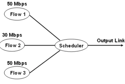
Bandwidth Sharing is defined as the maximal data rate that is available for the flow. Consider the case of bandwidth sharing shown in Figure 3.1 where a scheme aims at achieving 50, 30, 50 Mbps when the optimal that can be achieved is 50, 10, 10 Mbps.
Figure 3.1: Example of bandwidth sharing.
3.4.2
Packet Delay
Packet Delay can be defined as the elapsed time for a packet to transit the network segment or a networking device.
ITU-T defines the QoS Metrics for delay as:
• IP packet transfer delay (IPTD): IP packet transfer delay is defined for all successful and error packet outcomes. If the packet is fragmented, the value corresponds to the last fragment.
• Mean IP packet transfer delay: Mean IPTD is the arithmetic average of IPTD for a population of interest.
On the other hand, IETF provides two definitions of packet delay:
• One-way Delay Metric for IPPM [15]: This is one of the basic quantitative characteristics of network delay. The metric is defined as the difference between wire-time of first bit of the Type-P packet at the transmitter and wire-time of the last bit at the receiver. The metric involves an upper bound of delay and considers that packet lost and the value of metric undefined if the last bit does not arrive within that predefined period of time. If the packet is fragmented and if, for whatever reason, reassembly does not occur, the packet will be deemed lost. Note that measuring one-way delay requires clock synchronization between the sender and receiver.
The delay experienced by packet k in a queue can be defined as :
dNk =|DNk −ANk| (3.1) where, AN
k ,DNk anddNk denote the arrival time, departure time and queuing delay of
packet k in queue N.
3.4.3
Delay Jitter
Packets sent on a packet switched network are most often delivered irregularly to the destination due to some of the reasons discussed in Section 3.3. Particularly in the case of real-time applications, this variation in network transfer delay (at network-level) or packet departure delay from a network device (at a system network-level) can cause degradation of quality of service. Additionally, bursty traffic patterns increase the delay jitter of a flow.
Two kinds of jitter play a major role in network QoS, delay jitter and rate jitter. Delay jitter bounds the maximum difference in the total delay of different packets arriving at a destination, assuming that the packet source is perfectly periodic. Rate jitter bounds the difference in packet delivery rates at various times. This is measured as the difference between the minimal and maximal inter-arrival times (inter-arrival time between packets is the reciprocal of rate) [17]. Both these measures are very useful for real-time voice and video applications. For the purpose of this study, we will be focus on delay jitter performance metrics.
Several definitions for delay jitter have been defined, of which two are discussed here [18]. The first measure is called2-point PDV (Packet Delay Variation), as defined by ITU-T SG13 in Rec.I.380 [19]. The 2-point packet delay variation (vk) for an IP
packet k between the source SRC and the destinationDST is the difference between the absolute IP packet transfer delay(xk) of the packet and a defined reference IP
packet transfer delay d1,2, between those same measurement points.
vk =xk−d1,2 (3.2)
The reference IP packet transfer delay, d1,2, between the source and the destination
two measurement points[18]. Alternatively, the first packet delay can be replaced with average delay of the population of packets.
The second measure, called 1-point CDV (Cell Delay Variation), was defined by IETF [20], particularly for ATM environments. According to this definition, the vari-ation of delay is derived from the arrival time of cells, measured against an expected arrival time. Supposing a stream of cells transmitted with constant period T, the 1-point CDV of the cell k is the difference yk between the actual arrival time ak and
a reference time ck. The reference time (expected arrival time) is defined as follows:
c0 = 0 (3.3)
a0 = 0 (3.4)
If ck≥ak, (3.5)
then ck+1 =ck+T (3.6)
else ck+1 =ak+T (3.7)
Based on the 1-point CDV, the delay jitter of a packet k in a queue [20] can be defined as the difference of queuing delay of this packet and the preceding packet in that queue, i.e.,
jk =|dk−dk−1| (3.8)
wheredk is the queuing delay of packet number k. Additionally, we define the
aggre-gate jitter experienced by all packets that have been served by a queueN at a point in time τ as the sum of the jitter of each packet served by queueN from time 0 toτ, i.e.
javg(τ) = τ
t=0
|dNk −dNk−1| (3.9)
=
τ
t=0
|(DNk −DNk−1)−(ANk −ANk−1)| (3.10) (3.11)
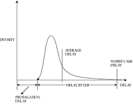
There has been a lot of research focusing on estimating the maximum delay jitter bound Jmax for different types of packets [21] and for variable packet sizes. Verma,
Zhang and Ferrari [22] discuss the feasibility of bounding the delay jitter in real-time channels and control of delay jitter in real-time communication in packet switched networks. Figure 3.2 gives an idea of the bounds on delay distribution curve [23].
Figure 3.2: Understanding Delay and Delay Jitter.
3.4.4
Packet Loss
Packet loss is the term given to losing information packets for a flow. Packet loss may happen in a flow due to:
• High input rate leading to queue overflow.
• Corruption of packets.
• Re-ordering within the flow.
Packet loss directly affects the reliability of the connection. Excess packet loss results in a less reliable connection.
• IP packet loss ratio (IPLR): IP packet loss ratio is a ratio of total lost IP packet outcomes to total transmitted IP packet in population of interest.
IP LR= Nlost
Ntransmitted
(3.12)
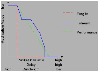
The applications can react on packet loss in three different ways [24].
1. Fragile: An application is unreliable if the packet loss exceeds certain threshold.
2. Tolerant: Multiple packet loss threshold levels are defined. The application can tolerate packet loss upto a particular level, but the higher the packet loss, the application is less reliable.
3. Performance: The application can tolerate even very high packet loss ratio but its performance can be very low in high packet loss ratio.
Figure 3.3: Loss graph
• IP packet error ratio (IPER): IP packet error ratio is the ratio of total errored IP packet outcomes to the total of successful IP packet transfer outcomes plus errored IP packet outcomes in a population of interest. This metric is usually defined in terms of Bit Error Rate (BER) or Frame Error Rate (FER).
IP ER= Nerroneous
Nerroneous+Nsuccessf ul
• Type-P One-way Packet Loss (IETF) [25]: IETF defines a packet loss metric for IPPM,Type-P One-way Packet Loss. The packet is considered lost if it fails to arrive to its destination in a reasonable period of time. This time threshold is a parameter of the metric. Corrupted packets are counted as lost. The measurement methodology relies on the one-way delay.
An example of an scheduling algorithm that takes packet loss into consideration is DWCS orDynamic Window-Constrained Scheduling. DWCS was originally designed to be network packet scheduler limiting the number of late or lost packets over a window-size of packets in loss-tolerant and/or delay-constrained heterogeneous traffic streams [26].
Service classes, discussed earlier in this chapter, represent a set of traffic types that demand specific packet delay, loss and jitter characteristics from the network on a per-hop basis. Networking applications with similar characteristics and performance requirements fall into the same service class and similar metric bounds.
We considered the quantitative metrics so far. Some of the other qualitative QoS parameters that may be considered for metrics are Cost, Compliance, and Security [27].
3.5
Fairness Index
3.5.1
Jain’s Fairness Index
ATM Forum Traffic Management Specification version 4.0 [28] defines a fairness index, called Jain’s fairness index, to evaluate the fairness of the distribution of the available bandwidth among the individual flow. Consider a scheduling algorithm allocating its output bandwidth to N flows. If xi is the observed throughput in the
i−th flow (where 0 ≤ i ≤ N) and ri is the expected throughput or fair share for
connection i (i.e., ri can be defined as an equal share of the bottleneck link capacity
ri = Capacity of Output Link/N), then Jain’s fairness index [29] is defined as:
F
x0 r0,· · ·,
xN
rN
=
(
i=0N −1) xi ri
2
n(i=0N −1)(xi
ri)2
(3.14)
Jain’s fairness index produces a normalized number between 0 and 1, where 0 indicates the greatest unfairness and 1 indicates the greatest fairness. Lets consider Jain’s fairness index for the example shown in Figure 3.1. The scheme gives 50, 30, 50 Mbps, when the optimal is 50, 10, 10 Mbps. Let the measured throughput be t1, t2,..., tn. Use any criterion (e.g., max-min optimality) to find the fair throughput p1, p2,..., pn [30].
Normalized Throughput: xi =
ti
pi
Fairness Index = (
(xi))2
nx2i
Example: 50/50, 30/10, 50/10 = 1,3,5
Fairness Index = (1 + 3 + 5)
2
3(12 + 32 + 52)
= 92
3(1 + 9 + 25) = 0.81
• Scalability: It can be applied to any number of flows. Fairness index like co-variance is not defined for small n. Performs really well for large number of flows.
• Scale independent: Jain’s index is independent of the scale. Additionally, Jain’s Fairness Index is a generic metric that can be applied to any resource.
• Bounded : Jain’s Fairness index always lies between 0 and 1 or 0 and 100. Variance, standard deviation, and relative distance are not bounded.
• User perception: Jain’s index has an easier user perception. Higher value of this index implies more fairness. Other indices like variance do not have this, as higher variance means less fairness
Chapter 4
Packet Scheduling Algorithms
Various scheduling algorithms and methods have been studied extensively in the literature. In this chapter, we summarize a few of them, that we have simulated for this research. In the first section, we start with an example of an ideal scheduling algorithm, the Generalized Processor Sharing algorithm, before describing other al-gorithms [33], [34], [35]. We then discuss Weighted Jitter EDF, a modification to the Earliest Deadline First (EDF) algorithm.
4.1
Background Work
4.1.1
Generalized Processor Sharing (GPS)
Generalized Processor Sharing or GPS is an idealized fluid flow scheduling model deploying uniform network resource sharing to achieve QoS guarantees such as fair bandwidth allocation and end-to-end delay bounds in communication networks. GPS is a work-conserving scheduler in which all the participating connections are simulta-neously provided with their fair service share.
with each of the flows. A GPS scheduler is one for which,
Si(τ1, τ2)
Sj(τ1, τ2) ≥
wi
wj
(4.1)
for each backlogged flow i, j in the interval τ1 to τ2. Summing over all flows j we get,
Si(τ1, τ2)
j
wj ≥(τ2−τ1)Rwi (4.2)
Hence, flow iis guaranteed a minimum fair share rate gi equal to
gi =
wi
jwj
R (4.3)
In other words, the service that a flow receives in a GPS system is no worse that an equivalent dedicated link with a capacity of gi (as shown in Eq.4.3).
Parekh and Gallager [37] show a clear example of how the flexibility of GPS multiplexing can be used effectively to control packet delay when combined with appropriate rate enforcement.
GPS is considered an ideal scheduling algorithm due to some of its unique prop-erties.
• Property 1: Let us define ri to be the average rate of flow i. Then, as long
as ri ≥ gi, the flow can be guaranteed a throughput of ρi independent of the
demands of the other flows. In addition to this throughput guarantee, backlog in flow i will always be cleared at a rate greater thangi.
• Property 2: The delay of an arriving flow i bit can be bounded as a function of the flow i queue length, independent of the queues and arrivals of the other flows.
• Property 3: By varying the wi’s, we have the flexibility of treating the flows in
a variety of different ways. For example, when all wi’s are equal (say equal to
1), the system reduces to uniform processor sharing.
ri =
R
As long as the combined average rate of the sessions is less thanR, any assign-ment of positive wi’s yields a stable system. For example, a high-bandwidth
delay-insensitive flowi can be assigned gi much less than its average rate, thus
allowing for better treatment of the other flows.
• Property 4: Most importantly, it is possible to make worst-case network queuing delay guarantees when the sources are constrained by leaky buckets.Thus, GPS is particularly attractive for flows sending real-time traffic such as voice and video.
Although GPS has these attractive properties, it is not implementable due to two main reasons. GPS works under the assumption that the scheduler can serve multiple flows simultaneously and that the traffic is infinitely divisible according to Eq. 4.3. Secondly, GPS is an idealized scheme which does not transmit packets as entities; it rather treats them as infinitesimal quantities. Both these assumptions do not hold in practice, since only one flow can be served by a scheduler at a given time, and an entire packet has to be served before serving another packet. However, GPS serves as a good scheme to compare and evaluate other scheduling disciplines.
4.2
Weighted Jitter Deadline Scheduling
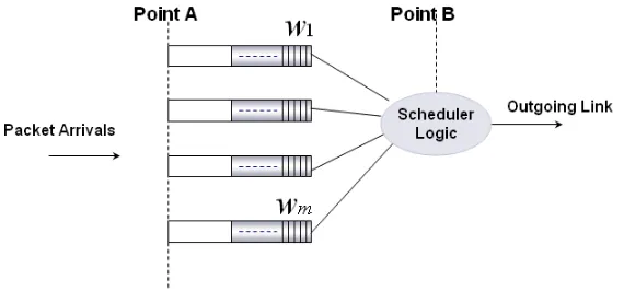
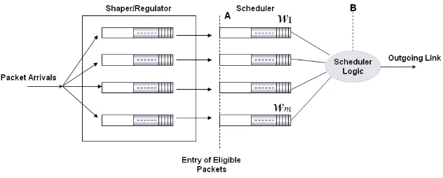
In this section, we discuss a simple scheduling algorithm called Weighted Jitter Earliest Deadline First Scheduling or WJ-EDF, a modification of Earliest Deadline First scheduling policy [38], designed with a focus to reduce the delay jitter expe-rienced by packets in output buffer schedulers [39]. A work-conserving scheduler is the most appropriate for an output buffer scheduler as it significantly decreases the average end-to-end delay experienced by packets and helps in the fair distribution of available bandwidth between competing flows.
Figure 4.1: Simple WJ-EDF scheduler
priorities to the m queues, different weights are assigned to the m queues, namely
w1, w2, w3,· · ·, wm. The weights are chosen in such a way that the queue which is the
least delay and jitter-tolerance must be given the highest weight value.
It is important to timestamp packets in any deadline-based scheduling policy. Integer timestamping is one possibility which is used in the implementation of this algorithm, discussed in section 5.2. The advantage of using integer timestamps as op-posed to floating-point timestamps is that integer timestamps have simpler hardware implementations. Aggregate jitter used in this algorithm is implemented according to the definition in section 3.4. The applicability of WJ-EDF has been studied for two categories of output buffer schedulers [39], namely Simple WJ-EDF Schedulers and Shaped WJ-EDF Schedulers.
4.2.1
Category 1 : Simple WJ-EDF
Figure 4.1 shows a structure of an output buffer-scheduler module where this algorithm can be applied. This algorithm is applied at two parts of the module,
• at point A, when packets enter the output buffers
On arrival of a packet or a cell k at entry point A in queue i, packets are times-tamped with an entry timesk
i. The deadlinefikof packetkin the queueiis calculated
as
fik=ski +dki (4.5)
where dk
i is the delay bound allowable for packet k.
According to [40], [41], and [42], EDF is known to be an optimal scheduling algo-rithm at a switch. Optimality is defined in terms of the schedulable region associated with the scheduling policy [41]. Consider m connections with traffic envelopes Ri(t),
(i= 1,2, . . . , m), sharing an output link of rate C. Suppose that each of the m con-nections has an upper bound, di, on the scheduling delay that packets from that
connection can tolerate; these bounds define a vector d = (d1, d2,· · ·, dm). Then the
scheduling region of a scheduling disciplineφis defined as the set of all vectorsd that are schedulable under φ. It has been proven in [43], [44] that EDF has the largest schedulable region of all scheduling disciplines under the condition
m
i=1
Ri(t−di)≤Ct (4.6)
where traffic is assumed to be fluid and Ri(t) = 0, ∀t <0.
In this algorithm, we will define dk
i =f(lki, Ri, wi) where Ri is the input rate for
flow iwith packet k of length lki. More specifically,
dki =
lk i
Ri·wi
(4.7)
Using the input rate considers the peak requirement on the flow and sets a tighter bound on the delay.
Algorithm on arrival of a new packet k in flow i
1. Timestamp the newly arrived packet with an entry time sk
i
2. Compute the deadline fk
i of packet k in queue i
fik=ski +( l
k i
Ri ·wi
)
At point B, the scheduler algorithm checks all the backlogged queues and looks for the head-of-line packet which has the earliest deadline (i.e., lowest timestamp) and starts transmitting packets in order of increasing deadline. Every queue maintains a log of the aggregate jitter, ji experienced by the packets it transmitted. Hence, every
queue has an estimate of the service that has provided to it. When a bias condition occurs, i.e., when two queues Qr and Qs have the same deadline, the priority is given
to the queue with a highest aggregated jitter value , based on the “greedy-choice” property, i.e., the decision point in the algorithm is based on what seems best at the moment.
WJ-EDF Algorithm to select the next packet to be scheduled
1. Extract the deadline of all backlogged queues
2. Sequentially check all the backlogged queues whose head-of-line
packet has the smallest deadline
3. If two flows i and j have the same deadline, select the flow
with greater value ofji.
4. Complete scanning all the backlogged queues.
5. Retrieve the head-of-line packet from the high priority queue
obtained in Step 1-4 and transmit.
This algorithm works most appropriately for small packets or when large packets are fragmented into smaller blocks as the delay bound considered in Eq.4.7 does not take into consideration the time taken to enqueue or dequeue a large packet. Ideally, it would be appropriate to timestamp a large packet when its boundary just enters point A and delay bound must completely take into account the time that will be taken by a big packet to leave the queue. However, with a small packet, the enqueue-dequeue time is small and can be considered negligible.
4.2.2
Category 2: Shaped WJ-EDF
Figure 4.2: Shaped WJ-EDF scheduler structure.
eligible for transmission, the packets are sent to the scheduler. All packets waiting to become eligible for transmission wait in the shaper, which is like a waiting room, which in most implementations, is a non-work conserving scheduler. Once the packets are eligible, they are transferred to the output buffers to be scheduled to the output link. Definition of eligibility of a packet to leave the regulator or shaper to be transmitted on the output link varies is based on the implementation of the shaper being delay-jitter or rate-delay-jitter based.
Combining shaping and scheduling changes the arrival pattern of the packets en-tering the scheduler. Understanding the arrival patterns of packets into the scheduler based on the traffic type supported can help optimizing the algorithm further. Adding a shaper to the scheduler does not degrade the behavior of the combined module, it only decreases the jitter and the delay experienced by the outgoing packets. There may be multiple variations in the implementation of the eligibility criteria of packets. For example, consider the example of a system receiving IP-AAL5-ATM packets. The shaper may send ATM cells that are eligible to the scheduler.The total jitter during the transmission of an IP packet is hence a function of the jitter experienced by the cells carrying this IP packet. Another variation of implementation of eligibility crite-ria, is the scenario where a large IP packets is fragmented into smaller fragments to aid efficient scheduling. Eligible fragments are then sent to the scheduler. Modifications can be made to the algorithm to accommodate such fragmentation.
fragments K” in packet k is computed as
K” =l
i k
pk
(4.8)
The algorithm on arrival of a fragment of a packet k can be modified to the following:
WJ-EDF Algorithm on arrival of a new packet k in flow i
1. Timestamp the newly arrived packet with an entry time ski
2. Compute the deadline fk
i of packet k in queue i
fik=ski +( p
k i
Ri ·wi
)
3. Enqueue the packet k in queue i
The aggregate jitter experienced in transmission of packet k is defined as as
jki =
K”
n=1
jni (4.9)
Bias conditions may occur when two flows have the same deadline. Under such bias conditions, the flow with the higher value of aggregate jitter is selected in order to help the higher jitter flow to reduce its jitter.
WJ-EDF has a delay bound close to or better than EDF. The better delay bounds are obtained by appropriately scaling the weights w1, w2,...,wm.
Chapter 5
Simulation Study
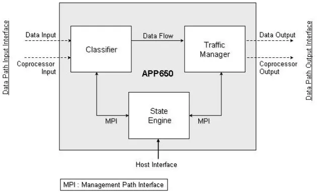
In this chapter, we discuss the implementation of packet scheduling schemes and the simulation study that was performed on Agere’s APP650 network processor. We start our discussion with a brief overview of the APP650 architecture, followed by a description of the simulation environments, the experiments we performed to compare the scheduling algorithms and the results of the simulations.
5.1
Architecture Overview
Advanced Payload Plus, APP650, is Agere’s third generation network processor and the simulations for this study were performed on its architecture . APP650 is a pipelined, multi-threaded processor that simultaneously analyzes and classifies multiple packets at the same time, monitors data traffic and schedules output data traffic, all at wire speed, operating at a clock rate of 266MHz. It includes sophisti-cated scheduling and shaping capabilities to support both packet or cell-based traffic. APP650 has integrated 10/100/1000 Ethernet MACs and provides flexible interface options including GMII/SMII (with integrated Gigabit Ethernet, 10/100 MACs), PMA (Gigabit Ethernet), SPI-3 and UTOPIA.
Figure 5.1 gives a high level system view of APP650’s architecture. The major components of the APP650 architecture include the following: