Estimating Nitrogen Efficiency of Swine Lagoon Liquid Applied to Field Crops Using Continuously Variable Irrigation

(1)

ABSTRACT

COBB, CHESTER RAY. Estimating nitrogen efficiency of swine lagoon liquid applied to field crops using continuously variable irrigation. (Under the direction of Robert L. Mikkelsen).

(2)

(3)

(4)

BIOGRAPHY

(5)

ACKNOWLEDGEMENTS

As I have endeavored the rigors of research and education in the pursuit of a Master of Science degree, I have been blessed in so many ways that I know I will forget something or even worse, somebody. First of all, I must give all glory and praise to God for He has always been there for me, leading the way when I have allowed Him to. Secondly, I am very grateful to Dr. John L. Havlin and the Soil Science Department at North Carolina State University for granting me a research assistantship so I could pursue a Master of Science degree. Without the financial support, I could not have returned to school on a full time basis. Also, I am very grateful for the guidance and encouragement from my advisor, Dr. Robert Mikkelsen. Not only did he guide me, but he also helped with the fieldwork. I am also thankful for Dr. Rod Huffman and his guidance with the irrigation design and Dr. Larry King for his input concerning the field design and measurement of residual soil N. Also, worth mentioning is Dr. Dan Israel who provided vital assistance for measuring the response of soybean to SLL additions.

(6)

(7)

LIST OF TABLES

Page Table 2.1 Manufacturer performance data of impact sprinklers considered

for utilization in the line-source irrigation technique ...26 Table 2.2 Summary of sprinkler locations and application conditions for

each irrigation event...30 Table 2.3 Estimated ammonia volatilization losses from sprinkler irrigation

of SLL ...40 Table 3.1 First-year N availability coefficients for swine manure based on

collection and application method ...50 Table 3.2 Nitrogen equivalency of SLL applied by irrigation as compared to

NH4NO3...90

Table 5.1 First-order model estimates for mineralized N accumulation from four field soils with a history of SLL applications and a nearby

unfertilized pine forest in 2000...128 Table 5.2 Summary of weekly inorganic N accumulation means from the

four field soils and a nearby pine forest soil from the 0 to 0.15 m

depth in 2000 ...131 Table 5.3 Summary of weekly inorganic N accumulation means from the

four field soils and a nearby pine forest soil from the 0.15 to 0.3

m depth in 2000 ...131 Table 5.4 Trends found for the changes in soil inorganic N within the

growing season ...136 Table 5.5 Partial N budget for SLL applied by irrigation in Section 2

compared to fertilizer N treatments in 1999 ...138 Table 5.6 Partial N budget for SLL applied by irrigation in Section 2

compared to fertilizer N treatments in 2000 ...139 Table A.1 Data collected for the pattern determinations of sprinkler

70CW-TNT shown in Fig. 2.3 ...147 Table A.2 Data collected for the pattern determinations of sprinkler

(11)

Table A.3 Data collected for the pattern determinations of sprinkler

7525-1-1M at 621 kPa shown in Fig. 2.5 ...149

Table A.4 Irrigation depths for June 7, 1999 for both SLL and water applications ...150

Table A.5 Irrigation depths for June 23, 1999 for both SLL and water applications ...151

Table A.6 Irrigation depths for July 28, 1999 for both SLL and water applications ...152

Table A.7 Irrigation depths for May 18, 2000 for water application...153

Table A.8 Irrigation depths for May 19, 2000 for SLL application ...154

Table A.9 Irrigation depths for June 2, 2000 for SLL application ...155

Table A.10 Irrigation depths for June 3, 2000 for water application...156

Table A.11 Irrigation depths for June 12, 2000 for SLL application ...157

Table A.12 Irrigation depths for June 12, 2000 for water application...158

Table A.13 Irrigation depths for July 21, 2000 for SLL application ...159

Table A.14 Irrigation depths for July 21, 2000 for water application ...160

Table A.15 Soil inorganic N concentrations measured in the spring of 1999 ...161

Table A.16 Soil inorganic N concentrations measured in the fall of 1999...162

Table A.17 Soil inorganic N concentrations measured in the spring of 2000 ...163

(12)

LIST OF FIGURES

Page Fig. 2.1 An example of a line-source sprinkler irrigation system design using

a sprinkler with a wetted diameter of 55 m and a sprinkler spacing

20% of the wetted diameter ...22 Fig. 2.2 Field layout of treatments at the Upper Coastal Plain Research

Station (Field P7) ...28 Fig. 2.3 Average radial distribution for 70CW-TNT at sprinkler pressures

(a) 580 kPa, (b) 440 kPa, and (c) 470 kPa ...32 Fig. 2.4 Average radial distribution for 80E-TNT at 520 kPa with (a)

spreader nozzle and (b) without spreader nozzle...33 Fig. 2.5 Average radial distribution for part circle impact sprinkler

(7525-1-1M) at 621 kPa...33 Fig. 2.6 Irrigation distribution for events A, B, and C in 1999...35 Fig. 2.7 Irrigation distribution for events D, E, F, and G in 2000 ...36 Fig. 2.8 Theoretical and actual distribution of combined water and SLL

applications for Event F...38 Fig. 2.9 Average N applied from SLL for all transects for irrigation events

A, B, and C in 1999. ...41 Fig. 2.10 Average N applied from SLL for all transects for irrigation events

D, E, F, and G in 2000 ...42 Fig. 2.11 Estimated N applied from SLL during irrigation Event F...43 Fig. 3.1 Monthly rainfall distribution during 1999 and 2000 at the Upper

Coastal Plain Research Station near Rocky Mount, NC...51 Fig. 3.2 Chlorophyll meter readings of the corn ear leaf in (a) 1999 and (b)

2000 as influenced by SLL additions in Section 1 and fertilizer

applications in Section 3 ...58 Fig. 3.3 Chlorophyll meter readings of the corn ear leaf in (a) 1999 and (b)

2000 as influenced by SLL additions in Section 2 and fertilizer

(13)

Fig. 3.4 Chlorophyll meter readings of the corn ear leaf in (a) 1999 and (b) 2000 as influenced by NH4NO3 additions and increases in water

irrigation depths in Section 3 ...61 Fig. 3.5 Corn ear leaf N concentrations in (a) 1999 and (b) 2000 as

influenced by SLL additions in Section 1 and fertilizer applications

in Section 3 ...62 Fig. 3.6 Corn ear leaf N concentrations in (a) 1999 and (b) 2000 as

in Section 3 ...63 Fig. 3.7 Corn ear leaf N concentrations in (a) 1999 and (b) 2000 as influenced

by NH4NO3 additions and increases in water irrigation depths in

Section 3 ...65 Fig. 3.8 Chlorophyll meter readings of the corn ear leaf as a predictor of leaf

N concentrations in 1999 and 2000 for (a) Section 1, (b) Section 2,

and (c) Section 3 ...67 Fig. 3.9 Corn yields in (a) 1999 and (b) 2000 as influenced by SLL additions

in Section 1 and fertilizer applications in Section 3 ...68 Fig. 3.10 Corn yields in (a) 1999 and (b) 2000 as influenced by SLL additions

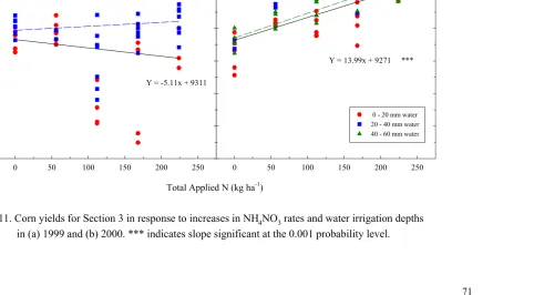
in Section 2 and fertilizer applications in Section 3 ...69 Fig. 3.11 Corn yields for Section 3 in response to increases in NH4NO3 rates

and water irrigation depths in (a) 1999 and (b) 2000 ...71 Fig. 3.12 Soybean (SB) and nonnodulating soybean (NSB) yields in (a) 1999

and (b) 2000 as influenced by SLL additions in Section 1 and

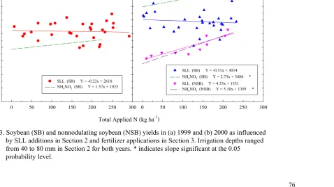
fertilizer applications in Section 3 ...75 Fig. 3.13 Soybean (SB) and nonnodulating soybean (NSB) yields in (a) 1999

and (b) 2000 as influenced by SLL additions in Section 2 and

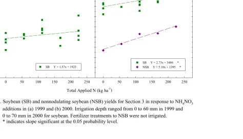
fertilizer applications in Section 3 ...76 Fig. 3.14 Soybean (SB) and nonnodulating soybean (NSB) yields for

Section 3 in response to NH4NO3 additions in (a) 1999 and (b)

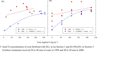
2000 ...77 Fig. 3.15 Seed N concentrations of corn fertilized with SLL in (a) Section 1

and (b) NH4NO3 additions in Section 3 ...80

(14)

Fig. 3.17 Seed N concentrations from soybean (SB) and non-nodulating soybean (NSB) in response to SLL additions in Section 1 and

NH4NO3 applications in (a) 1999 and (b) 2000...82

Fig. 3.18 Seed N concentrations from soybean (SB) and non-nodulating soybean (NSB) in response to SLL additions in Section 2 and

NH4NO3 applications in (a) 1999 and (b) 2000...83

Fig. 3.19 Removal of grain N by corn and soybean (SB) in 1999 from SLL additions in (a) Section 1 and (b) NH4NO3 applications in

Section 3 ...84 Fig. 3.20 Removal of grain N by corn and soybean (SB) in 1999 from SLL

additions in (a) Section 2 and (b) NH4NO3 applications in

Section 3 ...85 Fig. 3.21 Grain N removal by corn, soybean (SB), and non-nodulating

soybean (NSB) in 2000 from SLL additions in (a) Section 1 and

(b) NH4NO3 applications in Section 3 ...87

Fig. 3.22 Grain N removal by corn, soybean (SB), and non-nodulating soybean (NSB) in 2000 from SLL additions in (a) Section 2 and

(b) NH4NO3 applications in Section 3 ...88

Fig. 4.1 Fresh nodule mass from soybean roots in (a) 1999 and (b) 2000 as influenced by SLL additions in Section 1 and fertilizer applications

in Section 3 ...103 Fig. 4.2 Fresh nodule mass from soybean roots in (a) 1999 and (b) 2000 as

in Secton 3 ...104 Fig. 4.3 Influence of increasing NH4NO3 rates and water irrigaton depths on

fresh nodule mass in (a) 1999 and (b) 2000...105 Fig. 4.4 Acetylene reduction activity of soybean nodules in (a) 1999 and (b)

2000 as affected by SLL additions in Section 1 compared to

fertilizer applications in Section 3 ...108 Fig. 4.5 Acetylene reduction activity of soybean nodules in (a) 1999 and (b)

2000 as affected by SLL additions in Section 2 compared to

fertilizer applications in Section 3 ...109 Fig. 4.6 Acetylene reduction activity of soybean nodules in (a) 1999 and (b)

2000 as affected by increasing NH4NO3 rates and water irrigation

(15)

Fig. 4.7 Total acetylene reduction activity of soybean nodules as reflected

by nodule mass...111 Fig. 4.8 Estimation of N2 fixation reduction in (a) 1999 and (b) 2000 from

additions of SLL in Section 1 compared to fertilizer applications in

Section 3 ...113 Fig. 4.9 Estimation of N2 fixation reduction in (a) 1999 and (b) 2000 from

additions of SLL in Section 2 compared to fertilizer applications in

Section 3 ...114 Fig. 4.10 Estimation of N2 fixation reduction in (a) 1999 and (b) 2000 as

affected by increasing NH4NO3 rates and water irrigation depths ...115

Fig. 5.1 Cumulative N mineralized in the upper 0.15 m of soil from the

research plots and a nearby pine forest ...126 Fig. 5.2 Cumulative N mineralized from soil in the research plots and a

nearby pine forest at the 0.15 to 0.30 m depth...127 Fig. 5.3 Net change in soil inorganic N by depth within the growing season

in Section 1 for corn, soybean, and nonnodulating soybean (NSB)

receiving SLL ...133 Fig. 5.4 Net change in soil inorganic N by depth within the growing season

receiving SLL and irrigation water...134 Fig. 5.5 Net change in soil inorganic N by depth within the growing season

(16)

LIST OF ABBREVIATIONS

Abbrev. Meaning

C2H2 Acetylene

C2H4 Ethylene

NCCES North Carolina Cooperative Extension Service

NSB nonnodulating soybean

NUE nitrogen use efficiency

PAN plant-available nitrogen

SB nodulating soybean

Section 1 received only swine lagoon liquid

Section 2 received both swine lagoon liquid and water

Section 3 received NH4NO3 treatments and variable amounts of water

SLL swine lagoon liquid

SPAD Soil Plant Analysis Development (chlorophyll meter unit of measurement)

(17)

CHAPTER 1 GENERAL INTRODUCTION

North Carolina is recognized as one of the leading swine (Sus scrofa domesticus) producing states in the nation. In 1999, receipts from swine production were second to broilers in North Carolina with approximately $1.2 billion generated (NASS, 2000). As the revenue from swine production has increased, swine farms have grown in size while decreasing in number. In North Carolina, approximately 640 of the 3,680 swine farms accounted for 76% of the hogs and pigs inventory in 2000 (North Carolina Agriculture and Consumer Services, 2001). The trend to fewer and larger swine farms has been influenced by the integration and specialization of swine production in the United States (Mikkelsen, 2000).

While integration and specialization of swine farms have improved production efficiencies (McBride, 1995), other issues such as animal welfare and waste management have received more attention. A major concern for waste management has been the amount of waste generated within a localized area. While swine manure is a valuable fertilizer for crop production, the amount of waste generated may provide more nutrients than crops grown on the farm can utilize. The value of swine manure is reduced as distance from the source increases due to handling difficulties, transportation costs, and the availability of relatively inexpensive inorganic fertilizers.

(18)

Alabama use some type of lagoon system (Liu et al., 1995). In North Carolina, 85% of the swine farms utilize some type of lagoon system for waste treatment (Barker and Zublena, 1995).

Anaerobic lagoons provide partial waste treatment by reducing nutrient content and biological activity prior to land application. Within an anaerobic lagoon, some of the organic matter is converted into methane. As methane and other organic gases diffuse into the atmosphere from the lagoon, the O2 demand is reduced by 75 to 85%

(Mikkelsen, 2000). Nitrogen is removed from the anaerobic lagoon liquid through NH3

volatilization. Mikkelsen (1997) estimated volatilization losses to be as high as 50 to 75% of the N entering the lagoon. Much of the P entering the lagoon settles with the sludge at the bottom. While some waste treatment occurs in the lagoon, the liquid is often further treated by disposal onto cropland.

(19)

Nitrogen Content of Anaerobic Swine Lagoon Liquid

Nitrogen concentrations of anaerobic swine lagoons vary depending on animal factors (breed, age, size, gender, etc.), housing environment, and feed composition (Mikkelsen, 2000). From three similarly operated swine lagoons, Wilhelm et al. (1980) found total N concentrations ranged from 309 to 938 mg N L-1. While total N concentrations vary between lagoons, research has indicated that the majority of the N is in the inorganic form. Zublena et al. (1990) estimated that out of 60 kg ha-cm-1 (136 lb acre-inch-1) of total N for anaerobic SLL, 80% of the total N is present as NH4+.

Chescheir et al. (1985) reported NH4+–N concentrations from SLL that were 82 and

92% of the total N. Other research (Westerman et al., 1995; Evans et al., 1984; Safley et al., 1992) has reported that 70 to 90% of the N in SLL is present in ammoniacal forms. While these concentrations can be used for N estimates from anaerobic swine lagoons, laboratory analysis of the SLL is needed for accurate N determinations on individual farms.

Plant Uptake

(20)

Coastal bermudagrass (Cynodon dactylon L. Pers.) is often used as a receiver crop for SLL applications because its high nutrients requirement (NCCES, 1997). Burns et al. (1990) applying SLL to bermudagrass at 1, 2, and 4 times recommended N rates (335 kg ha-1), reported plant N recoveries of 72, 74, and 44% respectively. In another experiment, bermudagrass removed about 60% of the applied N (435 kg ha-1) from SLL (Westerman et al., 1995). Finally, when SLL was applied by irrigation to tall fescue (Festuca arundinacea L. Schreb) for 4 years at approximately 600 and 1,200 kg N ha-1 yr-1, plant N removal at the end of the 4 years accounted for 64 and 35% of the total N applied respectively (Westerman et al., 1987).

Pathways of N loss, mainly NH3 volatilization, denitrification, and NO3

-leaching, lower plant uptake of applied N (Wiesler, 1998). In an experiment in Indiana, Sutton et al. (1995) compared corn utilization of applied N from equivalent rates of swine manure and anhydrous NH3 injected into 4 different soils. Similar corn yields

were obtained with equal rates of swine manure and anhydrous NH3 for all soils when a

(21)

Mineralization

Mineralization is important because it is the process by which organic forms of N are converted to inorganic NH4. This reaction requires heterotrophic soil

microorganisms that use the organic N compounds as an energy source for their metabolism. For optimum mineralization within the soil, a temperature range of 40 to 60 oC and a moisture content that is 50 to 75% of the soil’s water holding capacity is required (Sims, 1995). Given optimum environmental conditions, the amount of C in respect to the amount of N present generally determines the rate of mineralization.

Flowers and Arnold (1983) evaluated the effects of adding 100 µg NH4+–N g-1

(22)

Nitrification

The oxidation of NH4+ to NO3- by autotrophic and heterotrophic bacteria is

referred to as nitrification. Assuming a sufficient population of nitrifying bacteria, the amount of NH4+ present, soil pH, presence of O2, soil moisture, and temperature are the

primary factors influencing nitrification rates. Generally, environmental conditions capable of supporting crop growth are also favorable for nitrification. Xu et al. (1998) used irrigation to apply SLL to corn in order to validate a computer model prediction of daily N2O emissions. The highest N2O emission rates occurred one day after SLL

application. Because the amounts of N2O emitted were proportional to the amounts of

NH4+ in the SLL, they determined that N2O emissions within one day after application

were released by nitrification. This suggests that NH4+ added to the soil can be nitrified

within a few days after application under favorable conditions.

Volatilization

Ammonia volatilization and denitrification are pathways of gaseous N losses to the atmosphere. Because of the high NH4+ content of SLL, NH3 volatilization tends to

be high for SLL applied by irrigation. The extent of NH3 volatilization is determined by

the difference in NH3 partial pressure between the ambient atmosphere and that in

equilibrium with the solution (Peoples et al., 1995). The NH4+ concentration, solution

temperature, and pH of the effluent or soil solution are important factors that affect the partial pressure of NH3 and thus NH3 volatilization.

Obviously, materials with higher NH4+ concentrations have the potential for

(23)

temperature of the solution. As temperature increases, the relative proportion of NH3 to

NH4+ at a given pH increases (Peoples et al., 1995). This shift in temperature decreases

the solubility of NH3 in water and allows for greater NH3 diffusion into the atmosphere.

Ammonia volatilization is also enhanced with increases in the pH of the solution. The equilibrium between NH4+ and NH3 in solution is affected by the pH of

the solution. As pH increases from 6 to 7, 8, and 9, the relative NH3 concentration

increases from 0.1 to 1, 10, and 50% respectively (Peoples et al., 1995). Higher NH3

concentrations potentially lead to increased NH3 volatilization. Pote et al. (1980) in an

experiment evaluating NH3 losses during sprinkler application of SLL predicted NH3

losses to be ≤8% when the pH of the SLL was near neutral (7 to 8). At a pH of 10.5, they estimated NH3 losses of 30 to 60% for sprinkler irrigated SLL. Pote et al. (1980)

also evaluated NH3 losses during sprinkler irrigation of SLL considering the size and

flight of a spray droplet. They noticed that NH3 losses from SLL at pH 10.5 were <50%

when droplet diameter was >2 mm and >50% when droplet diameter was <2 mm.

Various amounts of NH3 volatilization during sprinkler irrigation of SLL have

been reported. Burns et al., (1987) evaluated SLL applications to tall fescue and observed that NH3 losses from nighttime sprinkler irrigation events averaged 10%

during the spring and 22% during the summer. In another study using nighttime sprinkler irrigation, Humenik et al. (1976) reported a NH3 loss of 25% during

(24)

slight decrease in NH3–N concentrations between the liquid collected during irrigation

and the lagoon liquid was noticed, they determined that volumetric losses during irrigation accounted for 62 to 100% of the NH3. Evaporation and droplet drift lowered

the amount of liquid collected during irrigation.

Not only is NH3 lost during irrigation, but it is also lost from the surface of

plants and the soil after SLL applications. No research was found documenting NH3

losses from the surface of plants after SLL applications. Volatilization of NH3 from the

soil is affected by crop cover and application method. Peoples et al. (1995) reported that NH3 losses ranged from 9 to 33% of the fertilizer N when applied to grasslands and

range from negligible to >50% when applied to upland and lowland cropping systems. Hoff et al. (1981) found that injection of liquid swine manure led to lower NH3 losses

from the soil when compared to broadcast applications of liquid swine manure. When liquid swine manure was injected into the soil at rates of 205 and 409 kg NH4–N ha-1,

2.5% of the total applied N was lost as NH3. On the other hand, when liquid swine

manure was surface applied at the same rates, the amount of NH3 lost was 14 and 11.2%

respectively. Sharpe and Harper (1997) measured NH3 losses totaling 82% from SLL

applied to oat (Avena sativa) by irrigation, of which 69% was NH3 volatilization from

the soil. Based on previous research data concerning NH3 losses during irrigation of

(25)

Denitrification

The reduction of NO3- and NO2- into NO, N2O, and N2 is referred to as

denitrification. Anaerobic conditions are required for denitrification to occur. The amount of O2 present in the soil is primarily controlled by soil texture, structure, and

moisture content. Generally, denitrification can occur at soil moisture contents > 60% of the pore space (Peoples et al., 1995). Other factors influencing denitrification are pH, temperature, and the amount of soluble organic C. The pH and temperature range required for most field crops is favorable for denitrification. Soluble organic C is required to provide the energy source and electrons for the reducing bacteria.

Peoples et al. (1995) reported denitrification losses ranging from 2 to 9% when N fertilizer was applied to a well-drained sandy loam soil. When N fertilizer was applied to a poorly drained sandy loam soil, denitrification losses ranged from 6 to 30%. Thompson et al. (1987) recorded denitrification losses of 12 and 2% for cattle slurry N surface applied to grassland when applied in December and April respectively. Over a period of 15 days starting at the first irrigation event and ending one day after the last irrigation event, Sharpe and Harper (1997) measured N2O emissions that accounted for

about 13% of total N additions from three applications of SLL onto oats. No attempt was made to determine what percentage of the N2O emissions were derived specifically

from denitrification or nitrification.

(26)

was found to be the major mechanism for NO3–N loss in the poorly drained soil

compared to leaching for the moderately well-drained soil. Favorable conditions for denitrification were found in the poorly drained soil from 1.2 to 2.1 m below the soil surface throughout the year. The water table generally ranged from 0.3 to 0.6 m below the surface for the poorly drained soil during the winter and early spring and generally remained below 3.5 m for the moderately well-drained soil. Evans et al. (1995) summarized studies examining the impacts of different drainage systems on surface water quality in the Coastal Plain of North Carolina. They reported that in some cases NO3–N concentrations were reduced by 10 to 20% in the outflow from controlled

drainage (allows shallow water table management) as compared to conventional drainage (only promotes water movement away from the field). Denitrification was believed to be the major pathway for the loss of NO3–N in those cases. Kliewer and

Gilliam (1995) reported higher denitrification rates as the water table was maintained nearer to the soil surface. The majority of denitrification occurred within 36 to 54 cm of the soil surface when the water table was maintained at either the 30 or 45 cm depth. When the water table depth was maintained at 15 cm, denitrification shifted from the 36 to 54 cm zone to the 18 to 36 cm zone as NO3–N was depleted at the lower depth.

(27)

Leaching

Leaching is the process by which nutrients are lost as water percolates through the soil profile. Nitrate is susceptible to leaching because it is an anion and is not attracted to the cation exchange sites in the soil. Leaching of NO3- to the aquifers or to

surface waters such as rivers and lakes is a concern for several reasons (NCCES, 1997; Westerman et al., 1995). The maximum allowable concentration for NO3- in drinking

water is 10 ppm or mg L-1 NO3–N as established by the United States Public Health

Service (1962). Eutrophication may become a problem when nutrients, such as N, are present in excessive concentrations in surficial waters (NCCES, 1997).

Most studies have documented NO3–N accumulations in soil profiles at

excessive manure application rates (King et al., 1990; Westerman et al., 1995; Westerman et al., 1987; Evans et al., 1984; Humenik et al., 1976). Patni (1995) showed that animal manure slurry applied at rates of 500 kg N ha-1 yr-1 to field crops for more than 4 years led to NO3–N concentrations >10 mg L-1 in subsurface drainage waters.

These concentrations persisted for several years after applications had stopped. Similar NO3–N concentrations have also been found in the shallow groundwater below

agricultural fields receiving inorganic fertilizers (Evans et al., 2000). When SLL was applied at recommended rates to coastal bermudagrass grown on a sandy soil, Westerman et al. (1995) found that three sampling wells outside of the plots had NO3–N

(28)

highest application rate showed NO3–N concentrations increasing from about 5 to 20 µg

g-1 as soil depth increased from 0 to 90 cm. Soil cores taken 1.8 m downslope from the plots showed NO3–N increasing up to about 10 µg g-1 to a soil depth of 90 cm. Sloan et

al. (1999) found elevated NO3- concentrations in the shallow groundwater beneath a

bermudagrass spray field. The pasture had been used for a spray field for about 20 years and during the study received approximately 350 to 400 kg N ha-1 yr-1. Occasionally, concentrations in excess of 40 mg NO3–N L-1 were found in wells

immediately adjacent to the nearby stream. It appears that significant leaching of NO3

-occurs when excessive amounts of SLL are applied onto agricultural fields and when a spray field receives annual applications of SLL for many years. These same trends could also be expected from N fertilizer when applied in excess of the plant requirement.

Runoff

(29)

study, the months with the highest rainfall had the highest runoff. Finally, Westerman et al. (1985) reported that the greatest potential for high concentrations of waste constituents in runoff is during irrigation events and when irrigation occurs during rainfall events. Increasing application rates of SLL had little effect on the quantity runoff. In most of the cases above, irrigation rates were applied to supply a certain amount of N. No consideration was given to rainfall in respect to irrigation events. As a result, irrigation events sometime occurred during rainfall events or even when rain was predicted. Thus, with proper irrigation management, N losses through runoff can be controlled.

Immobilization

Immobilization is the reverse of mineralization and it involves the assimilation of inorganic N by soil microbes into organic compounds that constitute microbial biomass. Nitrogen is immobilized as a microbial population grows to decompose organic matter (C). Optimum soil conditions for immobilization are similar to those required for mineralization (Sims, 1995). Of the physical and chemical properties of the organic waste, the C to N ratio (C:N) is one of the most important factors in predicting immobilization. Sims (1995) reported that organic wastes with high C:N ratio (C:N > 25:1) provide high-energy sources for microbes causing immobilization of the inorganic N.

(30)

temperatures >5oC, there were no differences in N amounts immobilized over the range of temperatures (5 – 30oC) tested. Overall, they reported that net immobilization occurred within 30 days after application and approximately 40% of the NH4–N in the

pig slurry was immobilized. In a study looking at SLL applied to bermudagrass hay fields, Aho (1996) recorded a higher potential for N immobilization in the pasture with a loam texture than the pasture with a loamy sand texture. Ammonium concentrations in the loamy sand soil increased by 51% of the applied N compared to about 10% for the loam after SLL application. The increased immobilization potential for the loam was related to higher dissolved organic C concentrations found in the loam than the sandy loam. Thus, the amount of N immobilized is highly influenced by the C:N ratio of the material and the amount of C in the soil. Since SLL has a low C:N ratio, approximately 0.5:1 (Barker et al., 1994), the soil properties of the spray field would have the largest effect on the rate of immobilization.

Conclusions

(31)

REFERENCES

Aho, D.W. 1996. Nitrogen transformations and loss in pastures receiving swine lagoon liquid. Ph.D. diss. North Carolina State Univ., Raleigh, NC.

Andreadakis, A.D. 1992. Anaerobic digestion of piggery wastes. Water Sci. Technol. 25:9–16.

Barker, J.C. and J.P. Zublena.1995. Livestock manure nutrient assessment in North Carolina. p. 98–106. In C.C. Ross (ed.) 7th International Symposium on Agricultural and Food Processing Wastes. ASAE Chicago, IL.

Barker, J.C., J.P. Zublena, and C.R. Campbell. 1994. Livestock manure production and characterization in North Carolina. North Carolina State Univ., Raleigh, NC. Burns, J.C., L.D. King, and P.W. Westerman. 1990. Long-term swine lagoon effluent

applications on ‘coastal’ bermudagrass: I. Yield, quality, and element removal. J. Environ. Qual. 19:749–756.

Burns, J.C., P.W. Westerman, L.D. King, M.R. Overcash, and G.A. Cummings. 1987. Swine manure and lagoon effluent applied to a temperate forage mixture: I. Persistence, yield, quality, and elemental removal. J. Environ. Qual. 16:99–105. Chescheir, G.M., P.W. Westerman, and L.M. Safley. 1985. Rapid methods for

determining nutrients in livestock manures. Trans. ASAE 28:1817–1824. Evans, R.O., J.P. Lilly, R.W. Skaggs, and J.W. Gilliam. 2000. Rural land use, water

movement, and coastal water quality. North Carolina Cooperative Extension Service. Publ. #AG-605. North Carolina State Univ., Raleigh, NC.

Evans, R.O., R.W. Skaggs, and J.W. Gilliam. 1995. Controlled versus conventional drainage effects on water quality. J. Irrig. and Drain. Eng. 121:271–276.

Evans, R.O., P.W. Westerman, and M.R. Overcash 1984. Subsurface drainage water quality from land application of swine lagoon effluent. Trans. ASAE 27:473–480. Flowers, T.H. and P.W. Arnold. 1983. Immobilization and mineralization of nitrogen in

soils incubated with pig slurry or ammonium sulphate. Soil Biol. Biochem. 15:329–335.

Gambrell, R.P., J.W. Gilliam, and S.B. Weed. 1975. Denitrification in subsoils of the North Carolina Coastal Plain as affected by soil drainage. J. Environ. Qual. 4:311–316.

(32)

Humenik, F.J. and M.R. Overcash. 1976. Design criteria for swine waste treatment systems. EPA-600/2-76-233. Robert S. Kerr Environmental Research Laboratory. U.S. Environmental Protection Agency, Ada, OK.

King, L.D., J.C. Burns, and P.W. Westerman. 1990. Long-term swine lagoon effluent applications on ‘coastal’ bermudagrass: II. Effect on nutrient accumulation in soil. J. Environ. Qual. 19:756–760.

Kliewer, B.A. and J.W. Gilliam. 1995. Water table management effects on

denitrification and nitrous oxide evolution. Soil Sci. Soc. Am. J. 59:1694–1701. Liu, F.H., C.C. Mitchell, D.T. Odom, and E.W. Rochester. 1995. Nitrogen in surface and seepage water from overland flow of swine lagoon effluent. p. 170–184. In

C.C. Ross (ed.) 7th International Symposium on Agricultural and Food Processing Wastes. ASAE, Chicago, IL.

McBride, W.D. 1995. U.S. hog production costs and returns. 1992. An economic handbook. USDA Econ. Res. Serv. Rep. 724. U.S. Gov. Washington, D.C.

Mikkelsen, R.L. 2000. Beneficial use of swine by-products: opportunities for the future. p. 451–480. In J.F. Power and W.A. Dick (ed.) Land Application of Agricultural, Industrial, and Municipal By-Products. Soil Sci. Society of America. Madison, WI. Mikkelsen, R.L. 1997. Agricultural and environmental issues in the management of

swine waste. p. 110–119. In J.E. Rechcigl and H.C. MacKinnon (ed.) Agricultural Uses of By-products and Wastes. Am. Chem. Soc. Symp. Ser. 668. ASC,

Washington, D.C.

National Agricultural Statistics Service. 2000. Statistical Highlights 2000/2001. Statistical Bulletin 971. (Available on-line at http://www.usda.gov/nass/Pubs/ stathigh/content.html). (Verified 9 Sept. 2001).

North Carolina Agriculture and Consumer Services. 2001. Hogs and pigs: Number of operations [Online]. Available at http://www.ncagr.com/stats/livestoc/anihigyr.txt. (Verified 9 Sept. 2001).

NCCES. 1997. Certification training for operators of animal waste management systems – Type A. North Carolina Cooperative Extension Service. Publ. #AG-538-A. North Carolina State Univ., Raleigh, NC.

(33)

Peoples, M.B., J.R. Frenzy, and A.R. Mosier. 1995. Minimizing gaseous losses of nitrogen. p. 565–602. In P.E. Bacon (ed.) Nitrogen Fertilization in the

Environment. Marcel Dekker, Inc., New York, NY.

Pote, J.W., J.R. Miner, and J.K. Koelliker. 1980. Ammonia losses during sprinkler application of animal wastes. Trans. ASAE 23:1202–1212.

Safley, L.M., J.C. Barker, and P.W. Westerman. 1992. Loss of nitrogen during sprinkler irrigation of swine lagoon liquid. Biores. Technol. 40:7–15.

Skarda, M. 1977. Utilization of animal wastes for crop production. p. 315–327. In E.P. Taigamides (ed.) Animal Wastes. Applied Science Publishers, London.

Sharpe, R.R. and L.A. Harper. 1997. Ammonia and nitrous oxide emissions from sprinkler irrigation applications of swine effluent. J. Environ. Qual. 26:1703–1706. Sloan, A.J., J.W. Gilliam, J.E. Parsons, R.L. Mikkelsen, and R.C. Riley. 1999.

Groundwater nitrate depletion in a swine lagoon effluent-irrigated pasture and adjacent riparian zone. J. Soil Water Conserv. 54:651–656.

Sims, J.T. 1995. Organic wastes as alternative nitrogen sources. p. 487–535. In P.E. Bacon (ed.) Nitrogen Fertilization in the Environment. Marcel Dekker, Inc., New York, NY.

Sutton, A.L., D.M. Huber, B.C. Jeorn, and D.D. Jones. 1995. Management of nitrogen in swine manure to enhance crop production and minimize pollution. p. 535–540.

In C.C. Ross (ed.) 7th International Symposium on Agricultural and Food Processing Wastes. ASAE, Chicago, IL.

Thompson, R.B., J.C. Ryden, and D.R. Lockyer. 1987. Fate of nitrogen in cattle slurry following surface application or injection to grassland. Soil Sci. Soc. Am. J. 38:689–700.

United States Public Health Service. 1962. Drinking water standards. Publ. 956. Washington, D.C.

Westerman, P.W., R.L. Huffman, and J.C. Barker. 1995. Environmental and agronomic evaluation of applying swine lagoon effluent to coastal bermudagrass for intensive grazing and hay. p. 150–161. In C.C. Ross (ed.) 7th International Symposium on Agricultural and Food Processing Wastes. ASAE, Chicago, IL.

(34)

Westerman, P.W., M.R. Overcash, R.O. Evans, L.D. King, J.C. Burns, and G.A. Cummings. 1985. Swine lagoon effluent applied to ‘coastal’ bermudagrass: III. Irrigation and rainfall runoff. J. Environ. Qual. 14:22–25.

Wiesler, F. 1998. Comparative assessment of the efficacy of various nitrogen fertilizers. p. 81–114. In Z. Rengel (ed.) Nutrient Use in Crop Production. Haworth Press Inc. Binghamton, NY.

Wilhelm, R.G., D.C. Martens, D.L. Hallock, E.R. Collins Jr., and E.T. Kornegay. 1980. Characterization and agricultural utilization of swine waste lagoon effluents: Effects on growth of maize. Water Air Soil Pollut. 14:443–450.

Xu, C., M.J. Shaffer, and M. Al-kaisi. 1998. Simulating the impact of management practices on nitrous oxide emissions. Soil Sci. Soc. Am. J. 62:736–742. Zublena, J.P., J.C. Barker, and J.W. Parker. 1990. Soil Facts: Swine manure as a

(35)

CHAPTER 2 CONTINUOUS VARIABLE NITROGEN APPLICATIONS OF

SWINE LAGOON LIQUID ONTO FIELD CROPS USING THE

LINE-SOURCE IRRIGATION TECHNIQUE

ABSTRACT

(36)

INTRODUCTION

For most agronomic studies, crop response to essential plant nutrients is typically measured using 4 or 5 application rates of the nutrient in question. When the treatments are replicated and placed in a random block design, statistical analysis can show significant differences among treatments. However, the discrete treatments selected may not be appropriate for generating a response curve. The line-source irrigation technique incorporates continuously variable applications of the treatments with a relatively small land requirement.

The concept for the line-source irrigation technique originated from a continuous function experiment dealing with N fertilization of sweet corn (Fox, 1973). Individual plants were fertilized with urea from 0 to 220 kg ha-1 in 5.5 kg ha-1 increments. With this design, the N level increased in small increments in one direction. Fox suggested that a second factor such as irrigation could be added to the study interactions. In this case, the first factor is varied in one direction while the second factor is varied perpendicular to the first. A concern with Fox’s design was that plot size consisted of a single corn plant.

(37)

Hanks et al. (1976) designed a field irrigation study to obtain a continuously variable application pattern. This research design became known as the “line-source” sprinkler irrigation system. Very simply, this design involved a single line of sprinklers down the center of the plot (Fig. 2.1). Hence the identifier “line-source” was coined. To obtain the continuous “triangular” application pattern as a function of distance from the line-source, it was suggested that the sprinklers be spaced at 10% or less of the wetted diameter. This type of sprinkler spacing allowed for greater uniformity at application levels parallel to the line. However, often it is desirable to use wider sprinkler spacings due to material costs and the high application rates next to the line. It was suggested that sprinkler spacings up to 20 to 25% of the wetted diameter are reasonable as long as the variations in application depths parallel to the line do not exceed ±10% of the mean. Some of the limitations Hanks et al. (1976) observed with this research design were the distortions of sprinkler patterns due to wind speeds ≥3 km h-1), no variation in irrigation frequency allowed due to the structured irrigation levels, and problems with ponding or runoff that may occur at the highest application rates.

(38)

Fig. 2.1. An example of a line-source sprinkler irrigation system design using a sprinkler with a wetted diameter of 55 m and a sprinkler spacing 20% of the wetted diameter.

is obtained as sprinkler spacing decreases. While uniformity is desired, the application rate may exceed the infiltration capacity of the soil when sprinklers are spaced closer together.

(39)

however, irrigation effects are large enough that statistical analysis is not as critical. For the randomly applied variables, an analysis of variance does provide a valid error term. Bauder et al. (1975) conducted an experiment to observe differences between results obtained from a continuously variable plot design and a randomized block, split block design. The results from each experiment led to basically the same conclusions. Using data from three different experiments, Bresler et al. (1982) reported on spatial techniques to address the statistical problems arising from the continuous variable water applications. They used scaled variograms to filter out the trend imposed by the variable water amounts, thus revealing the influence of other factors assumed to be homogeneous such as soil properties and experimental errors. For every experiment they analyzed, the scaled variograms revealed that the average crop response within an irrigation level was strongly dependent on the amount of water received at that location. Their analysis also revealed that soil properties could significantly influence the variability of crop responses measured.

(40)

lettuce (Lactuca sativa L.) cultivars. Recently, Guttieri et al. (2000) used the line-source technique to determine the effects of moisture stress on the final quality (protein content, flour yield, and bread making quality) of six hard red spring wheat (Triticum aestivum L.) cultivars.

Also, the line-source concept has been used to supply variable rates of another factor such as N while eliminating the water gradient. Lauer (1983) modified the line-source concept to provide a variable N application rate along with a uniform water application. This was accomplished by adding two additional irrigation lines, one to each side of the main line-source. The N gradient was produced by injecting N into the irrigation system and distributing it through the middle line of sprinklers. The outer lines were used to equalize the applied water amounts to either side of the middle line. Building upon the design used by Lauer (1983), Magnusson et al. (1988) designed a study to simultaneously evaluate linear gradients of water, salinity, and N on corn growth and development. Their design involved two perpendicular sets of three irrigation lines. The centerline of one set was used to apply the N gradient while the centerline of the other was used to apply the saline water gradient. They demonstrated that decreasing concentrations gradients from the line-source could be produced for two variables without varying the water.

(41)

(1998) evaluated plant response to N and water from celery (Apium graveolens), broccoli (Brassica oleracea L.), and potato (Solanum tuberosum L.), respectively. All three of these studies determined water and N management needed for optimal vegetable production while minimizing the amount of N lost through leaching.

As documented, the line-source technique effectively provides variable gradients that can be used for many research applications. This present study adopts the line-source concept to provide variable applications of anaerobic SLL to field crops. Since the amount of N in the SLL is proportional to the liquid in the SLL, another line-source consisting of only water was added to eliminate the water gradient. The objectives of this study were to (1) determine sprinkler setup necessary for achieving variable SLL application amounts, (2) document SLL and water application amounts as distance from the irrigation line increased, and (3) determine the amount of N applied from the irrigated SLL.

MATERIALS AND METHODS

(42)

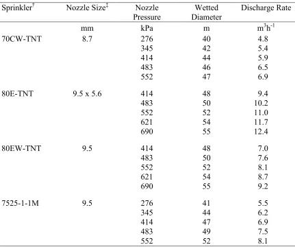
Table 2.1. Manufacturer performance data of impact sprinklers considered for utilization in the line-source irrigation technique.

Sprinkler† Nozzle Size‡ Nozzle Pressure

Wetted Diameter

Discharge Rate

mm kPa m m3h-1

70CW-TNT 8.7 276 40 4.8

345 42 5.4

414 44 5.9

483 46 6.5

552 47 6.9

80E-TNT 9.5 x 5.6 414 48 9.4

483 50 10.2

552 52 11.0

621 54 11.7

690 55 12.4

80EW-TNT 9.5 414 48 7.0

483 50 7.6

552 52 8.1

621 54 8.7

690 55 9.2

7525-1-1M 9.5 276 41 5.5

345 44 6.2

414 47 6.9

483 49 7.5

552 52 8.1

†_{Sprinklers 70CW-TNT, 80E-TNT, and 80EW-TNT are manufactured by Rain Bird.}

(Glendora, CA.). Sprinkler 7525-1-1M manufactured by Senninger (Orlando, Fl.). Use of these specific sprinklers is not meant as an endorsement.

‡_{Sprinkler 80E-TNT has a 5.6 mm spreader nozzle.}

Sprinkler Tests

(43)

basis. The radial profile was determined to be the average application depth at specific distances from the sprinkler. Next, the radial profile for the selected sprinkler was entered into a computer program, designed by R. Huffman (Biological and Agricultural Engineering Dept., NCSU), which calculates and displays the overlapped application pattern for arbitrary head spacings. By inspecting the program outputs, the sprinklers and head spacing that would provide the desired variable application pattern were selected.

Experimental Design

After sprinkler type and spacing had been selected, the field research plots were designed to fit sprinkler and field constraints (Fig. 2.2). A parallel water line-source was added to eliminate the water gradient from the SLL line-source. Based on the irrigation design, the field was divided into three blocks, 30 by 88 m each. Section 3 was increased by 6 m to provide a non-irrigated area. The area in which water and SLL applications overlapped was labeled as Section 2. Section 1 received only continuously variable SLL applications. Section 3 consisted of randomized fertilizer treatments with continuously variable water applications.

(44)

Fig. 2.2. Field layout of treatments at the Upper Coastal Plain Research Station (Field P7).

Irrigation Events

(45)

water, pump pressure, nozzle pressure, and wind speed were recorded periodically (Table 2.2).

For most irrigation events, 12 rows of 30 to 31 catch cans were placed in sets of three transects (along crop rows) perpendicular to the line-source. The first line of catch cans was in line with the centermost sprinkler with the other two lines placed 3 m and 6.1 m to the side of the sprinkler location. When a transect was in line with the sprinkler, the catch cans were spaced 1.5 m from the sprinkler and then every 3 m. The height of the catch cans was ≈1.2 m for soybean. For corn, average catch can height was ≈1.2 m in events A, D, and E and ≈2.1 m in events B, F, G, and H (Table 2.2). Maps of the irrigation distribution and variable N rate were generated in ArcView using the spline method to interpret the data.

Nitrogen Application Rates

The amount of N applied from SLL and water applications was based on N concentrations of random liquid samples taken from catch cans immediately after irrigation. Liquid samples were also taken directly from the line-sources as the irrigation system depressurized to determine N concentrations pumped from the lagoon. After collection, the samples were placed in a cooler with ice and transferred to a refrigerator (4oC) until they could be analyzed for N. Total N was measured by the macro-Kjeldahl method (APHA, 1992) using CuSO4 as the catalyst to convert organic

N into NH3–N. Once the N was converted to the NH3-N form, N was measured by

(46)

Table 2.2. Summary of sprinklers locations and application conditions for each irrigation event. Event†_{Date Liquid}

Irrigated Irrigation Run Duration of Sprinklers Used Sprinkler Locations

‡_Pump

Pressure Sprinkler Pressure SpeedWind § _DirectionWind

min Row # kPa kPa m s-1

A 7 June 1999 SLL * 80E-TNT 16, 43, 70, 83 * * 1.9–3.0 SW–WSW Water * 80E-TNT 9, 22, 36, 50, 63, 80 * *

B 23 June 1999 SLL 30 80E-TNT 16, 43, 70, 83 828 760 2.3–3.0 NE–ENE Water 30 80E-TNT 9, 22, 36, 50, 63, 80 828 690

C 28 July 1999 SLL 60 80E-TNT 14, 20 690 690 0.7 N

SLL 7525-1-1M 48 *

Water 60 80E-TNT (-5), 10, 23 690 690

Water 7525-1-1M 50 586

D 18 May 2000 Water 60 80E-TNT 75 760 760 4.2–5.1 SW

Water 70CW-TNT 83

Water 7525-1-1M 49, 96 690

19 May 2000 SLL 60 80E-TNT 75 655 655 4.6–5.1 SW–WSW

SLL 70CW-TNT 62

SLL 7525-1-1M 49, 96 620

E 2 June 2000 SLL 40 80E-TNT 22, 35, 49, 62, 76 620 620 1.6–2.2 WNW–NW

SLL 7525-1-1M 2, 96 620

3 June 2000 Water 40 80E-TNT 16, 29, 42, 55, 69, 83 690 590 1.1–3.9 N

Water 7525-1-1M 2, 96 590

F 12 June 2000 SLL 40 80E-TNT 22, 35, 49, 62, 76 760 725 2.5 WSW

SLL 7525-1-1M 2, 96 690

Water 45 80E-TNT 16, 29, 42, 55, 69, 83 760 690 1.8–2.7 SSW

Water 7525-1-1M 2, 96

G 21 July 2000 SLL 65 80E-TNT 22 690 690 0.9 NE

SLL 7525-1-1M 2, 42 690

Water 40 80E-TNT 22 790 760 0.6–1.4 NE–E

Water 7525-1-1M 2, 42 690

†_{Events C and J applied only to soybean. Events D and E applied only to corn. SLL and water applied simultaneously for events A, B, and C.} ‡_{Soybean start with row #1 and end with row #48. Corn starts with row #49 and ends with row #96. Row #(-5) is 5 rows outside row #1} §_{Wind data was collected from the weather station on the research farm as provided by the State Climate Office of North Carolina at NCSU.}

(47)

RESULTS AND DISCUSSION

Preliminary Sprinkler Tests

Very little change in the radial profile was noticed for the 70CW-TNT as sprinkler pressure increased from 440 to 580 kPa (Fig. 2.3). When the straightening vane was removed from the nozzle, the distribution pattern became smoother at a sprinkler pressure of 470 kPa (Fig. 2.3). A larger wetted diameter was obtained with sprinkler 80E-TNT (≈32 m) than 70CW-TNT (≈24 m) as indicated by the increase in radial distance (Fig. 2.4). When the spreader nozzle was removed from 80E-TNT and replaced with a plug, the radial profile was smoother (Fig. 2.4). However, there was more variability in the data for 80E-TNT without the spreader nozzle. Some of the enhanced variability may have been due to wind effect (0.9 – 2.7 m s-1) during the test. For the other reported tests, wind movement was minimal. Based on these results, sprinkler 80E-TNT was chosen over 70CW-TNT, in part because it covered a larger distance (wetted diameter) from the sprinkler. While a stronger triangular pattern was obtained for 80E-TNT with a spreader nozzle, 80E-TNT with the plug instead of the spreader nozzle was selected because of the lower application rates (Fig. 2.4).

(48)

Fig. 2.3. Average radial distribution for 70CW-TNT at sprinkler pressures (a) 580 kPa, (b) 440 kPa, and (c) 470 kPa. For sprinkler test (c), the straightening vane was removed from the nozzle. Error bar represents the standard deviation of the mean from all catch cans at a given distance from the sprinkler.

0 2 4 6 8 10

12

_(a)

A

ppl

ic

at

ion R

ate

(mm

h

-1 )

0 2 4 6 8 10 12

Distance From Sprinkler (m)

0 4 8 12 16 20 24

0 2 4 6 8 10 12

(b)

(49)

Fig. 2.4. Average radial distribution for 80E-TNT at 520 kPa with (a) spreader nozzle and (b) without spreader nozzle. Error bar represents the standard deviation of the mean from all catch cans at a given distance from the sprinkler.

0 2 4 6 8 10 12 14

0 4 8 12 16 20 24 28 32

A ppli cation R ate (m m h -1 ) 0 2 4 6 8 10 12 14 (a) (b)

Fig. 2.5. Average radial distribution for part circle impact sprinkler (7525-1-1M) at 621 kPa. Error bar represents the standard deviation of the mean from all catch cans at a given distance from the sprinkler.

0 5 10 15 20 25 30

(50)

Irrigation Events

A total of three irrigation events were applied in 1999 and four in 2000. The average application depths for catch cans locations in respect to line-sources were calculated for the entire field area (Fig. 2.6 and 2.7). The application depths for each experimental section (Fig. 2.2) are found at distances of 0 to 30 m for Section 1, 30 to 60 m for Section 2, and 60 to 90 m for Section 3 (Fig. 2.6 and 2.7). Fewer points are reported for Event D in 2000 (Fig. 2.7) because there were no catch can transects in line with the sprinklers. For the other irrigation events, there were at least two transects in line with the sprinklers. Irrigation Events A and B in 1999 and Events E and F in 2000 were applied to both corn and soybean. Events C in 1999 and G in 2000 were applied only to soybean. In 2000, Event D was applied to corn only.

(51)

Fig. 2.6. Irrigation distribution for events A, B, and C in 1999 (see Table 2.1 for details). Error bar represents the standard deviation of the mean from all catch cans at a given distance from the sprinkler.

0 10 20 30 40

Ir

ri

ga

tio

n D

epth

(

mm)

0 10 20 30 40

Distance (m)

0 10 20 30 40 50 60 70 80 90

0 10 20 30 40

SLL Line Water Line

A

B

(52)

Fig. 2.7. Irrigation distribution for events D, E, F, and G in 2000 (See Table 2.2 for details about the irrigation events). Error bar represents the standard deviation of the mean from all catch cans at a given distance from the sprinkler.

0 10 20 30 40

Irriga

tion Depth (mm)

0 10 20 30 40

Distance (m)

0 10 20 30 40 50 60 70 80 90

0 10 20 30 40

D

E

F

G

(53)

Irrigation distribution patterns appear to be more uniform at a given distance from the sprinkler in 2000 (Fig. 2.7) than 1999 (Fig. 2.6). The improved uniformity resulted from closer sprinkler spacing in 2000 (Table 2.1) and the use of the part circle impact sprinklers for increased coverage toward the ends of the line-sources. The part circle impact sprinklers were not used until Event C in 1999. Events D and G were more variable than events E and F in 2000 due to fewer sprinklers used. Fewer sprinklers were used for Events D and G because only corn or soybean was irrigated respectively. Irrigation depths ranged from 0 to 20 mm in Section 1 and 3 for Events E and F (Fig. 2.7). For Section 2, average depths ranged from 12 to 28 mm with the highest depths midway between the SLL and water line-sources. When only one crop was irrigated (Events D and G), depths ranged from 20 to 30 mm and the peak between the line-sources was less distinct (Fig. 2.7). Average irrigation depths for Sections 1 and 3 ranged from 0 to 30 mm for Events D and G.

(54)

(55)

Estimated Nitrogen Applied

Ammonia volatilization losses were calculated as the difference in total N concentrations of the pumped SLL and that of the SLL in the catch cans (Table 2.3). The amount of N applied from SLL was assumed to be the N content of the catch cans after irrigation as calculated by multiplying the average catch can N concentration by the SLL volume collected. Note that this calculation gives only an estimate of the total N applied because it does not include any further N losses that occur after irrigation. Less than 5 kg N ha-1 each year was added with the irrigation water itself.

(56)

Table 2.3. Estimated ammonia volatilization losses from sprinkler irrigation of SLL.

Nitrogen Concentration Event†

Start

Time Lagoon Catch cans‡

Estimated NH3 Loss

Sprinkler Pressure

Air Temperature§ (Initial – Final)

Relative Humidity§ (Initial – Final)

---mg N L-1--- % kPa oC %

A 7:00 a.m. 554 510 8.0 22 – 27 96 - 79

B 8:45 a.m. 464 437 6.0 760 21 – 23 86 - 78

C 7:20 a.m. 407 368 9.7 690 24 – 31 100 - 84

D 8:00 a.m. 566 527 6.8 690 23 – 27 70 - 56

E 8:10 a.m. 552 432 21.8 620 28 – 32 68 - 52

F 8:15 a.m. 508 442 13.0 725 24 – 27 72 - 66

G 6:50 a.m. 383 336 12.2 690 21 – 22 91 - 86

†_{Events A, B and C occurred in 1999 and the rest in 2000. See Table 2.1 for more information.} ‡_{Average concentration from random sampled catch cans.}

(57)

Fig. 2.9. Average N applied from SLL for all transects for irrigation events A, B, and C in 1999. Error bar represents the standard deviation of the mean from all catch cans at a given distance from the sprinkler.

0 20 40 60 80 100 120

A

pplied N

(k

g ha

-1 )

0 20 40 60 80 100 120

Distance (m)

0 10 20 30 40 50 60

0 20 40 60 80 100 120

SLL Line

A

B

(58)

Distance (m)

0 10 20 30 40 50 60

0 20 40 60 80 100 120 140 160

Fig. 2.10. Average N applied from SLL for all transects for irrigation events D, E, F, and G in 2000. Error bar represents the standard deviation of the mean from all catch cans at a given distance from the sprinkler.

(59)

(60)

CONCLUSIONS

(61)

REFERENCES

American Public Health Association. 1992. Standard methods for the examination of water and wastewater. 22nd Ed. Amer. Public Health Assoc., Washington, DC. American Society of Agricultural Engineers. 1999. Procedure for sprinkler distribution

testing for research purposes. ASAE Standards S491. ASAE, St. Joseph, MI. Bauder, J. W., R.J. Hanks, and D.W. James. 1975. Crop production function

determinations as influenced by irrigation and nitrogen fertilization using a continuous variable design. Soil Sci. Soc. Amer. J. 39:1187–1192.

Beverly, R.B., W.M. Jarrell, and J. Letey. 1986. A nitrogen and water response surface for sprinkler-irrigated broccoli. Agron. J. 78:91–94.

Bresler, E., G. Dagan, and R.J. Hanks. 1982. Statistical analysis of crop yield under controlled line-source irrigation. Soil Sci. Soc. Amer. J. 46:841–847.

Fox, R.L. 1973. Agronomic investigations using continuous function experimental designs – nitrogen fertilization of sweet corn. Agron. J. 65: 454–456.

Gallardo, M., L.E. Jackson, K. Schulbach, R.L. Synder, R.B. Thompson, and L.J. Wyland. 1996. Production and water use in lettuces under variable water supply. Irrig. Sci. 16:125–137.

Guttieri, M.J., R. Ahmad, J.C. Stark, and E. Souza. 2000. End-use quality of six hard red spring wheat cultivars at different irrigation levels. Crop Sci. 40:631–635. Hanks, R.J., G.L. Ashcroft, V.P. Rasmussen, and G.D. Wilson. 1978. Corn production

as influenced by irrigation and salinity – Utah studies. Irrig. Sci. 1:47–59.

Hanks, R.J., J. Keller, V.P. Rasmussen, and G.D. Wilson. 1976. Line source sprinkler for continuous variable irrigation-crop production studies. Soil Sci. Soc. Amer. J. 40:426–429.

Hanks, R.J., D.V. Sisson, R.L. Hurst, and K.G. Hubbard. 1980. Statistical analysis of results from irrigation experiments using the line-source sprinkler system. Soil Sci. Soc. Amer. J. 44:886–888.

Lauer, D.A. 1983. Line-source sprinkler system for experimentation with sprinkler-applied nitrogen fertilizers. Soil Sci. Soc. Amer. J. 47:124–128.

(62)

Meyer, R.D. and D.B. Marcum. 1998. Potato yield, petiole nitrogen, and soil nitrogen response to water and nitrogen. Agron. J. 90: 420–429.

Miller, D.E. and A.N. Hang. 1980. Deficit, high-frequency irrigation of sugarbeets with the line source technique. Soil Sci. Soc. Amer. J. 44:1295–1298.

Singh, R. and J. Singh. 1996. Irrigation planning in cotton through simulation modeling. Irrig. Sci. 17:31–36.

Sorensen, V.M., R.J. Hanks, and R.L. Cartee. 1980. Cultivation during early season and irrigation influences on corn production. Agron. J. 72:266–270.

Stark, J.C., W.M. Jarrell, and J. Letey. 1983. Evaluation of irrigation-nitrogen management practices for celery using continuous-variable irrigation. 1983. Soil Sci. Soc. Amer. J. 47:95–98.

(63)

CHAPTER 3 NITROGEN EFFICIENCY OF ANAEROBIC SWINE LAGOON

LIQUID APPLIED BY IRRIGATION TO FIELD CROPS

ABSTRACT

(64)

(65)

INTRODUCTION

Application of SLL onto agronomic crops by irrigation is the most common means of disposal because of the essential plant nutrients present. Bermudagrass (Cynodon dactylon), used either as hay or pasture, is the most common crop used as the receiver of the SLL. The high nutrient requirement, ease of management, and length of uptake period (from April to September) encourage the use of bermudagrass as a receiver crop for SLL (NCCES, 1990; Burns et al. 1990). However, when bermudagrass is grazed by cattle, the amount of nutrients removed is lower than when it is used for hay production. Also, due to the low economic value of bermudagrass hay within a region, hay bales may be left rotting along the field edge where the nutrients are ultimately returned back to the environment. Therefore grain crops such as corn and soybean may be a better receiver of SLL since the harvested grain is removed from the field and sold off the farm.

(66)

coefficient of 50% is used for SLL to be applied by irrigation, meaning that half of the total applied N will become available for plant uptake during the growing season. For environmental and economic reasons, this coefficient must be determined accurately. Based on these concerns and the need for information regarding application of SLL to grain crops, research was conducted to determine PAN of SLL applied to grain crops by irrigation. The objectives of this research were to (1) measure corn and soybean utilization of applied N from SLL in comparison to NH4NO3 and (2) determine PAN

from crop utilization comparisons of SLL to NH4NO3.

Table 3.1. First-year N availability coefficients for swine manure based on collection and application method†.

Collection Method Injection‡

Soil

Incorporation§ Broadcast Irrigation

Scraped paved surface – .6 .4 –

Liquid manure slurry .8 .7 .4 .3

Anaerobic lagoon liquid .9 .8 .4 .5

Anaerobic lagoon sludge .6 .6 .4 .4

†_{Obtained from Zublena et al. (1990).} ‡_{Manure injected directly into the soil.}

§_{Manure spread onto the soil surface and incorporated within 2 days.}

MATERIALS AND METHODS

(67)

wet periods. Based on soil samples sent to the North Carolina Department of Agriculture Agronomic Division, no additions of lime, P, or K were needed for either corn or soybean. In previous years, the field was planted in corn and SLL was applied at recommended agronomic rates of N.

Monthly rainfall amounts from the Research Station were recorded for 1999 and 2000 (Fig. 3.1). Rainfall was significantly higher during September 1999 because of hurricanes Dennis and Floyd. The field was flooded for several days immediately after hurricane Floyd.

Fig. 3.1. Monthly rainfall distribution during 1999 and 2000 at the Upper Coastal Plain Research Station near Rocky Mount, NC.

Month

Januar y

Feburar y

(68)

Experimental Design and Implementation

The experimental layout, Fig. 2.2 in Chapter 2, consisted of 48 rows of corn and 48 rows of soybean. The supply lines for the effluent and water sprinklers were laid perpendicular to the rows. Based on the maximum throw of the sprinklers, the water line was spaced 30m away from the effluent line. The rows were divided into three sections depending on the location of the supply lines for the sprinklers. Section 1 received only variable rates of SLL. Located between the SLL line and the water line, Section 2 received variable rates of SLL along with variable rates of water to balance the amount of liquid applied across the section. Section 3 consisted of randomized fertilizer treatments that received variable rates of water. Transects of catch cans were placed along the rows in conjunction with the location of the sprinklers to measure the amount of SLL and water applied. More details of the irrigation design are presented in Chapter 2.

(69)

During 2000, deer significantly reduced the vegetative growth of the nodulating soybean within Section 3. Aboveground biomass samples from Section 3 and Section 1 (no deer damage) at 6 and 8 weeks after planting were collected (1 m of row), dried, and weighed. The reduction in vegetation was 63 and 60% at 6 and 8 weeks respectively.

Nitrogen Applications

Section 1 and 2 received N from irrigation with SLL. Applied N was calculated for each irrigation event by measuring total Kjeldahl N from SLL samples and accounting for NH3 volatilization losses during irrigation. Details for N analysis are

given in Chapter 2.

Section 3 consisted of randomized NH4NO3 treatments of 0, 56, 112, 168, and

224 kg N ha-1 with continuously variable water amounts. Each treatment consisted of 9 rows 36 m in length, except for the nonnodulating soybean in 2000. The nonnodulating soybean fertilizer plots were adjacent to the soybean plot in Section 3 (see Fig. 2.2) and received no water through irrigation. Plot size for the nonnodulating soybean randomized fertilizer treatments was 4 rows 4.6 m long. In 1999, NH4NO3 was

broadcasted in two split applications using a drop spreader one month after corn planting (28 May) and one month later (23 June). In 2000, the NH4NO3 was banded by