Evaluation of Different Methods for Populating the LTPP Materials Database with the Dynamic Modulus

(1)

Kim).

The NCHRP 1-37A Guide for Mechanistic-Empirical Design of New and Rehabilitated Design Structures introduces the dynamic modulus (|E*|) as the material property to characterize asphalt concrete. This is a significant change from the resilient modulus (MR) used in the previous AASHTO Pavement Design Guide. One of the challenges of

changing the material characterization is that databases, such as the Long Term Pavement Performance (LTPP) Materials Database, contain older material characterization

information. Therefore, databases must be updated to the currently accepted standard. This thesis evaluates two methods to populate the LTTP database with |E*| values: 1) determine the |E*| from different geometries (i.e., cores and prisms) and 2) predicting the |E*| from the measured MR values in the database.

(2)

the |E*| experimentally, specifically from previously constructed pavements.

Practioners prefer a mathematical model since measuring the |E*| is a time and labor intensive. The second section of this thesis presents an artificial neural network (ANN) to predict the |E*| from the measured MR. The first step is an analytical method of

calculating the MR from the |E*|. It involves the application of multiaxial linear

viscoelastic theory to linear elastic solutions for the indirect tension test developed by Hondros (1959). The results show that the predicted and measured MR values are in close

agreement. The results provide a forward model for the back-calculation of the |E*| from MR. Using this forward model, a database of measured dynamic moduli is populated with

corresponding predicted resilient moduli to train an ANN. The trained ANN is the back calculation model used to predict |E*| from measured MR. The dynamic moduli predicted

(3)

By

Andrew Thomas LaCroix

A thesis submitted to the Graduate Faculty of North Carolina State University

In partial fulfillment of the Requirements for the Degree of

Master of Science

Civil, Construction, and Environmental Engineering Raleigh, North Carolina

2007

APPROVED BY:

____________________________ __________________________

Dr. Murthy N. Guddati Dr. Roy H. Borden

_________________________________ Dr. Y. Richard Kim

(4)

DEDICATION

This thesis is a testament to many people who have constantly encouraged me to stretch and grow as I have journied along my academic career.

The primary influence on my academic career is my parents, Michael and Carol LaCroix, who have shown me the joys of learning a multitude of topics. Probably the most important lessons were about my faith in God, which has given me the strength to keep moving even when it seemed all was lost.

Professors Fr. Thomas McShane and Dr. Michael Cherney in the Department of Physics at Creighton University have encouraged me to succeed and explore new topics such as cellular automata and encouraged me to branch out into engineering.

Dr. E. Terence Foster, a professor of Construction Systems in the College of Engineering at the University of Nebraska at Omaha who provided me with the

encouragement and guidance to use my physics background as a firm grounding for the applications of civil engineering.

(5)

BIOGRAPHY

Andrew LaCroix was born in Greensboro, North Carolina to Michael and Carol LaCroix. After nine months there, his family moved to Albemarle, North Carolina, where they lived for nine years. Then the family moved to Reading, Pennslyvania, living there three years. His family then moved to Omaha, Nebraska, where he lived for ten years. Living in the Heartland of America strongly shapes who he since he completed sixth through the completion of his undergraduate degree in Omaha. The attitude of someone from the Heartland is honesty, directness, and simplicity. His attitude toward life is generally relaxed with the belief that God will provide all his needs. He graduated from Omaha Central High School in May 2001 with honors. He then remained in Omaha to attend Creighton University to earn a Bachelor of Science in Physics magna cum laude in May 2005.

(6)

ACKNOWLEDGEMENTS

The most important person to acknowledge is my wife, Amanda. Without her

encouragement, patience with long and crazy hours, helping sieve, and watching movies at the CFL, the research for this thesis would not be possible. I also acknowledge my parents for their encouragement and understanding when I vented about the number of differents tasks I have done over the years.

A special thanks to Christopher Capp and Jessica Allison of Duke University for being my adopted brother and sister, especially the first year of graduate school.

The most critical group of people for accomplishing the research were my lab partners. Shane Underwood has been a great mentor, especially by challenging me to think about the problem differently and solving many mechanical problems, many times by opening the right drawer. Sangyum Lee has been a great friend who could make me smile when it was what I needed most. The graduate students of Dr. Kim’s, Tae Young Yun, Cheol Min Baek, Jae Jun Lee, Ju Sang Lee, Fadi Jadoun, and Ardalan Mosavi Khandan, are appreciated for providing encouragement and coffee throughout the research process. Several professors were instrumental in teaching me. Dr. Kim provided the needed guidance, encouragement, and big picture to complete the study. Dr. Ranji S. Ranjithan taught me the concept of ANN. Dr. Arellano guided me in using statistics to determine conclusions from a large database with several interactions.

(7)

LIST OF FIGURES

Figure 2.1 Graphical Represenation of E*. ... 6

Figure 2.2 Example of measured |E*| values at different frequencies and temperatures... 8

Figure 2.3 Example of a temperature shift factor curve... 10

Figure 2.4 Time-temperature shifted |E*| mastercurve. ... 10

Figure 2.5 Idealized steady-state stress and strain curves with phase angle. ... 12

Figure 2.6 Stress distribution in the IDT specimen subjected to a strip load. ... 16

Figure 4.1 (a) Surface-mounted LVDTs and (b) IDT test setup with SHRP LGD. ... 22

Figure 5.1 Log-log line-of-equality of SA and SI |E*| values for (a) S12.5C, (b) S12.5FE, (c) S12.5CM, and (d) S12.5C-AV-2. ... 29

Figure 5.2 Line-of-equality of SA and SI |E*| values for (a) S12.5C, (b) S12.5FE, (c) S12.5CM, and (d) S12.5C-AV-2. ... 30

Figure 5.3 Line-of-equality of RI and RP |E*| values for (a) S12.5C-AV+2 and (b) S12.5FE-AV+3. ... 34

Figure 6.1 Poisson’s ratio versus reduced time for S12.5C. ... 46

Figure 6.2 Average |E*| mastercurves: (a) in log-log scale and (b) in semi-log scale. .... 50

Figure 6.3 Strain comparison for ν = 0.20 at 5°C: (a) vertical and (b) horizontal. ... 53

Figure 6.4 Strain comparison for ν = 0.35 at 25°C: (a) vertical and (b) horizontal... 54

Figure 6.5 Strain comparison for ν = 0.45 at 40°C: (a) vertical and (b) horizontal... 55

Figure 6.6 Comparison of predicted and measured MR values: (a) S12.5C, (b) S12.5CM, (c) S12.5FE, and (d) B25.0C. ... 57

Figure 6.7 Line-of-equality graph for mixture and binder shift factors from FHWA study. ... 59

Figure 6.8 Line-of-equality graph of training data: (a) log-log and (b) arithmetic scales. ... 60

Figure 6.9. Line-of-equality graph of verification using Witczak data (a) log-log and (b) arithmetic scales... 62

(10)

LIST OF TABLES

Table 2.1 Geometry Coefficients ... 14

Table 3.1 Summary of Asphalt Mixtures ... 17

Table 4.1 Comparison of Loading Histories for IDT |E*| and MR... 24

Table 5.1 Summary of Completed Test and Specimen Fabrication Methods ... 26

Table 5.2 Statistical Results for Geometry Comparisons... 31

Table 5.3 Statistical Results for RVE and Non-uniform Stress... 33

Table 5.4 Statistical Results for Compaction and Anisotropy... 37

Table 6.1 Comparison of Predicted and Measured MR Values ... 56

(11)

CHAPTER 1 INTRODUCTION

In mechanistic or mechanistic-empirical pavement design and analysis methods, it is essential to know the properties of the layer materials. These material properties define a basic relationship between the stresses and strains in the various layers. The 1993

AASHTO Pavement Design Guide employs the resilient modulus (MR) as the material

property representing the stiffness characteristics of layer materials. The MR is defined as

the ratio between applied stress (σa) and recoverable strain (εr); that is,

a R

r

M σ

ε

= . (1.1)

Several testing standards have been developed for the determination of the MR of asphalt

concrete using the indirect tensile (IDT) test method (ASTM D4123, NCHRP 1-28, SHRP P-07, NCHRP 1-28A).

One of the major changes in the recently developed NCHRP 1-37A Guide for

Mechanistic-Empirical Design of New and Rehabilitated Design Structures, compared to the 1993 AASHTO Guide, is that the dynamic modulus (|E*|) is used as the material property to characterize asphalt concrete. This transition from MR to |E*| may make a

significant amount of the MR data that have been collected in state highway agencies

obsolete, unless a method to measure the |E*| from existing pavements is developed or a method to convert MR values to |E*| is developed. One good example of a database with

MR values obtained from numerous cores taken from in-service pavements is the Long

(12)

different geometries (i.e., cores and prisms) and 2) predicting the |E*| from the measured MR values in the database.

1.1 Measuring Dynamic Modulus with Different Geometries

The first major challenge to populating the LTPP materials database with |E*| is acquiring the material property from existing pavements. For example, the LTPP

materials database has cores from many different pavements, but many cannot be cut and cored to the standard dimensions for measuring |E*|. The AASHTO TP-62 standard decribes a method to determine the |E*| and phase angle of hot mix asphalt (HMA) specimens using an axial compression load. In the standard, a specimen is a cylinder 150 mm (about 6.0 in.) tall and 100 mm (about 4.0 in.) in diameter. The height is greater than some thin pavements, which means the specimen cannot be cored from the surface of the pavement. Also, thicker asphalt concrete pavements are usually composed of several layers (such as base, intermediate, and surface layers). These layers may have different |E*| values, so the ability to characterize the |E*| for each layer from these cores is questionable.

Kim et al. (2004) evaluates the possibility of using IDT testing to measure the |E*| of existing asphalt concrete pavements by comparing the |E*| values from the IDT tests against those from axial compression tests on standard cylinders. Twelve asphalt

(13)

and the resulting cross sections can be cut or cored into specimens similar to the axial specimens used in the AASHTO TP-62 standard. In light of this fact, a prismatic column (prism) geometry is also considered in this study.

Several challenges are addressed in Chapter Five to evaluate the possibility of accepting IDT and/or prism testing as an alternative to standard cylinder. Kim et al. (2004) recognized that two main differences exist between IDT and axial compression tests. One difference is the uniaxial stress state in axial compression versus the biaxial state of stress in IDT. The other difference is the relative directions of compaction and stress-strain analysis. For axial compression tests on specimens compacted by the Superpave gyratory compactor (SGC), the directions of compaction and stress-strain analysis are identical. On the other hand, SGC-produced IDT specimens are tested

perpendicular to the compaction direction. In an anisotropic mixture, the aggregate within a mixture tends to have certain orientations based on the method of compaction (Hunter

et al., 2004, Tashman et al., 2004). The anisotropic aggregate structures resulting from SGC compaction could affect the stress-strain analysis. Another source of anisotropy is the effect of SGC versus field compaction, because specimens for measuring |E*| for existing databases are removed from pavements in the field. The total difference between the field IDT and laboratory axial compression measurements could be due to the effect of anisotropy because of the differences in state of stress, different directions between the compaction and the stress-strain analysis, and/or the compaction method.

(14)

recommendations in a white paper by Schwartz (2004). Chapter Five of the thesis presents experimental results to determine whether the |E*| can be measured from different geometries and compaction methods, as well as possible limitations that might exist for implementing this method as a standardized test.

1.2 Predicting Dynamic Modulus from Resilient Modulus

The LTPP materials database can be populated with |E*| values in a less rigorous, though less accurate method than measuring |E*|. Practioners desire a model to predict |E*| since measuring |E*| is a time and labor-intensive process. Currently, several predictive models of |E*| exist, such as the Witczak model (Bari and Witczak, 2007) and the Hirsch model (Christensen et al., 2003). These models use a variety of inputs such as binder properties, HMA volumetrics, and aggregate information. One of the measured mixture properties available in the LTPP materials database is MR. Therefore, is important to develop a

relationship between MR and |E*| to populate the LTPP material database with reasonably

accurate values of |E*|. Such a method has further benefit since some asphalt materials and pavement analysis methods still require the MR as an input.

MR provides a snapshot of the material behavior under one loading history (i.e., a 0.1

second haversine loading followed by a 0.9 second rest period) at different testing temperatures (normally three temperatures at 5°, 25°, and 40°C). Most attempts to develop the relationship between MR and |E*| so far have been empirical in nature, such

(15)

2005). Zhang (1996) explored the possibility of characterizing the viscoelastic properties from MR tests using Fourier analysis. It was concluded that this type of analysis is

impractical due to: 1) the difficulty in solving a large number of variables and, 2) the limited range of results, providing slightly more time-temperature characterization than MR data. Another challenge is that Fourier analysis requires a loading and deformation

history for optimizing the viscoelastic parameters, which most databases do not contain. Therefore, any attempt to predict the |E*| from the MR is, at best, empirical in nature. The

hypothesis of this study is the prediction of the MR from the |E*| can be made using the

theory of viscoelasticity.

The sixth chapter of the thesis presents an analytical approach to predict the MR from

the |E*|. Experimental results provide evidence that the concept is valid. Because the MR

of asphalt concrete is normally determined using the IDT test, analytical, viscoelastic solutions are developed for the IDT test configuration. It involves the application of multiaxial linear viscoelastic theory to linear elastic solutions for the IDT test developed by Hondros (1959). Since the ultimate purpose of this study is to populate the LTPP materials database with |E*| values, the linear viscoelastic solution is used as a forward model (i.e., |E*| is used to predict MR) for the back-calculation of |E*| from MR.

Using the forward solution method, a database of measured dynamic moduli, such as the Witczak database, is populated with corresponding predicted resilient moduli to train an artificial neural network (ANN). Once a database is populated with predicted MR

(16)

to predict |E*| from measured MR. Further information regarding the use of neural

networks in pavement applications can be found in Xu et al. (2002).

CHAPTER 2 MATERIAL PROPERTIES

2.1 Dynamic Modulus (|E*|)

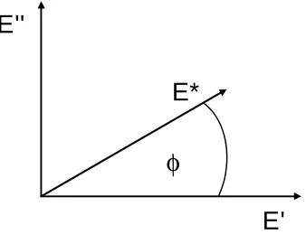
|E*| is one of the three fundamental material properties that can be used in the linear viscoelastic constitutive relationship. E* is the complex modulus, which is composed of the storage and loss modulus, as shown in Figure 2.1.

φ

E'

E''

E*

Figure 2.1 Graphical Represenation of E*. The complex modulus, E*, is represented as follows:

* ' "

E = +E iE , (2.1)

where

|E*| = magnitude of E*;

E' = storage modulus = |E*| cos φ; E" = loss modulus = |E*| sin φ.

The storage modulus represents the storage (elastic) component of energy of the

(17)

the relaxation modulus, E(t). Due to their fundamental nature, theoretical relationships exist among these three material properties that have been proven valid for the

characterization of asphalt concrete (Kim and Lee, 1995). The storage modulus (E’), can be represented in terms of a Prony series as seen in Equation (2.2). Knowing E’ is important for predicting the stress response to a given strain history.

2 2 2 2 1 '( ) 1 n

r i i r

i r i

E

E ω E ω ρ

ω ρ ∞

=

= +

+

∑

, (2.2)

where

E∞ = elastic modulus (MPa);

ωr = angular reduced frequency;

Ei = modulus of the ith Maxwell element; and ρi = relaxation time of the ith Maxwell element.

Since most |E*| tests are load-control tests, D(t) is needed to predict the strain response from a stress history. An exact conversion to D(t) can be obtained by solving the following equations:

[ ]

A D

{ } { }

= B , or AkjDj = Bk (2.3)

(

( / )

)

(

( / ) ( / )

)

1

1 k j k i k i

m

t i i t t

kj i j

i i j

E

A E e τ ρ e ρ e ρ ρ τ

ρ τ − − − ∞ = = − + − ≠ −

∑

, (2.4)

and

( / )

1 1

1 k i

m m

t

k i i

i i

B E_∞ E e− ρ E_∞ E

= =

   

= −_ + _{ } + _



∑

 

∑

. (2.5)

where,

Akj = matrix element in the kth row and jth column of matrix A;

(18)

E∞= equilibrium modulus (MPa);

Ei = modulus of the ith Maxwell element;

ρi = relaxation time of the ith Maxwell element determined a priori; τj = retardation time of the jth Voigt element determined a priori

tk = time of interest; and

m = number of Prony coefficients.

By solving for Dj, the Prony series representation for D(t) can be determined. Equation

(2.4) does not show a solution for ρi = τi since the error increases when such a case exists

(Park and Schapery, 1999).

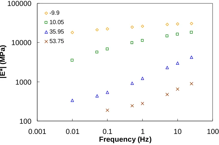
Since the behavior of viscoelastic materials is dependent on time, rate of loading, and temperature, these material properties are determined at multiple rates of loading and multiple temperatures (in degrees Celsius) as seen in Figure 2.2.

100 1000 10000 100000

0.001 0.01 0.1 1 10 100

Frequency (Hz)

|E

*|

(

M

P

a)

-9.9

10.05 35.95

53.75

(19)

A single, continous curve is developed using the time-temperature superposition

principle. The principle states that rheologically simple materials, such as HMA, can be shifted in the time or frequency domain (i.e., the horizontal axis) to produce a single, continuous curve. The equation for the shifted frequency, known as the reduced frequency, is:

r T

f =a f (2.6)

where

f = frequency (Hz); and fr = reduced frequency.

2

1 2 3

log(a_T)=a T +a T+a (2.7)

where

a1, a2, and a3 = coefficients; and

T = temperature.

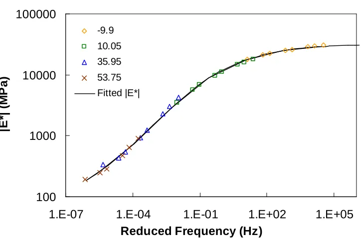
The |E*| values are shifted according to Equations (2.6) and (2.7) to produce a continuous curve called a mastercurve. Before shifting, a reference temperature is selected such that

log(aT) is zero. The result is a curve that provides the relationship between shift factors

(20)

y = 0.0006279x2 - 0.1576342x + 1.5907547 R2 = 0.9996966

-6 -5 -4 -3 -2 -1 0 1 2 3 4

-20 0 20 40 60

Temperature (C)

L

o

g

S

h

ift

F

a

c

tor

Figure 2.3 Example of a temperature shift factor curve.

100 1000 10000 100000

1.E-07 1.E-04 1.E-01 1.E+02 1.E+05 Reduced Frequency (Hz)

|E

*|

(

M

P

a)

-9.9

10.05

35.95 53.75

Fitted |E*|

(21)

As seen in Figure 2.4, the horizontal shifting of the |E*| values in Figure 2.2 produces a mastercurve. The mastercurve is represented by a sigmoidal function, Equation (2.8), which was selected to compensate for variability that might be present in the data.

*log( ) log | * |

1 1

r

c d f

b

E a

e + = +

+

, (2.8)

where

a, b, c, d = constants; and

fr = reduced frequency.

The reduced frequency represents the testing frequency needed to produce the |E*| value at the reference temperature. The benefit of time-temperature superpoisiton is the ability to predict the material response at temperatures and frequencies other than the measured values. To determine the |E*| at a different temperature and/or frequency, calculate the reduced frequency to find |E*| from the mastercurve sigmoidal equation.

2.1.1 |E*| Using Axial Compression

Axial compression is a uniaxial state of stress in the plane of loading. Axial and prism specimens are loaded in the uniaxial manner. Equation (2.9) shows the simple

formulation of calculating the |E*| from uniaxial measurements.

| * | o o

E σ

ε

= , (2.9)

where

(22)

The steady-state response of the material is a result of repeated sinusoidal loading. The following equation is used to calculate the steady-state response for stress and strain.

( ) cos( )

f t = + +a bt c ω φt+ (2.10)

where

f = stress of strain time history;

ω = angular frequency (radians/s);

φ = phase angle (radians); and

a, b, and c = fitting coefficients such that c is the stress or strain amplitude. Figure 2.5 shows a steady-state response for a stress and strain time histories. The dynamic modulus test described in AASHTO TP-62 is a load-controlled test, therefore the measured response is the deformation. The last five cycles are sampled to measure the amplitude and the phase angle between the stress and strain curves

-3 -2 -1 0 1 2 3

0 1 2 3 4 5

Time

S

tr

ess

o

r

S

tr

a

in

Load Strain

φ

σ

ο

ε

o

(23)

2.1.2 |E*| Using the IDT Test

IDT testing causes a biaxial state of stress in the plane of loading and the plane

perpendicular to it on the face of the specimen. Therefore, determination of |E*| from the IDT test requires a more complex formulation than uniaxial testing (e.g., AASHTO TP-62) requires. Drescher et al. (1997) and Zhang et al. (1997) applied the theory of

viscoelasticity to linear elastic solutions, developed by Hondros (1959), to develop linear viscoelastic solutions for stresses, strains, complex compliances, phase angle, and

Poisson’s ratio from the IDT test. The three-dimensional analysis includes calculations for deviatoric or shear stresses and volumetric stresses and strains (Drescher et al., 1997). To validate the solutions, the creep compliance from a creep test was used to calculate the horizontal and vertical displacements from a pulsed loading test, i.e., the MR test. Zhang et al. (1997) conclude that the viscoelastic solution predicted the displacements

reasonably well; they recommend a further step to validate the solution, which is to test more replicates at different temperatures.

(24)

multiple temperatures from the |E*| determined by the IDT test. In this study, the |E*| is calculated using the two-dimensional IDT derivation of Kim et al. (2004) since the MR is

calculated from two-dimensional elastic analysis.

1 2 2 1

2 2

2

* o

o o

P E

ad V U

β γ β γ

π γ β

− = −

− and (2.11)

1 1

2 2

o o

U V

β γ

ν

β γ

− =

− + , (2.12)

where

Po = applied load amplitude (N);

a = loading strip width (m); d = thickness of specimen (m);

Vo = amplitude of sinusoidal vertical displacement (m);

Uo = amplitude of sinusoidal horizontal displacement (m); and β1, β2, γ1, γ2 = geometric coefficients.

Table 2.1 Geometry Coefficients IDT |E*| β₁ β₂ γ₁ γ₂

-0.0134 -0.0042 0.0037 0.0116

MR k3 K4 k1 k2

-0.00067 0.000209 -0.00018 0.000578

The coefficients in Equations (2.11) and (2.12) are listed in Table 2.1. These

(25)

Therefore, in the IDT test, horizontal displacements are positive while vertical displacements and compressive loads are negative.

2.2 Resilient Modulus (MR)

MR can be calculated by several different methods, including the ASTM D 4123-82, the

NCHRP 1-28 method , the SHRP P07 protocol, AASHTO TP-31 standard, or the Roque and Buttlar equation (1992), which accounts for the bulging effects of the specimen. The NCHRP 1-28 elastic solutions are used in this paper. The equations for calculating MR

and Poisson’s ratio are given as follows:

1 2 (

R

P

M k k

Ud ν

= − ) and (2.13)

(

)

(

)

3 1

4 2

k k V U

ν = +

+ , (2.14)

where

MR = resilient modulus (MPa);

P = applied load (N);

d = thickness of specimen (m);

U = recoverable horizontal displacement (m); V = recoverable vertical displacement (m); and k1, k2, k3, k4 = constants.

Equations (2.13) and (2.14) can be combined to yield the following relationship:

(

)

(

)

3 1 1 2

4 2

R

k k V U

P

M k k

Ud k k V U

 + 

=  − ₊ 

 

(26)

These equations are based on the linear elastic solutions, developed by Hondros (1959), after accounting for the non-uniform stress and strain distributions in the IDT specimen, shown in Figure 2.6. The constants in Equations (2.13) and (2.14) are listed in Table 2.1. Note that these constants are different from the constants for |E*|, because the coefficients for MR are derived using linear elastic theory whereas those for |E*| are derived using

linear viscoelastic theory.

Y

sy

a

R 2a

P

sx

X

Figure 2.6 Stress distribution in the IDT specimen subjected to a strip load.

CHAPTER 3 MATERIALS AND SPECIMEN FABRICATION

The specimens in this study comprise ten different mixtures listed in Table 3.1. Five of these mixtures, S12.5C, S12.5CM, S12.5FE, S12.5F and B25.0C, have been provided by the North Carolina Department of Transportation. The first mixture is a surface mixture that has a 12.5 mm (0.5 in.) nominal maximum aggregate size (S12.5C) and coarse aggregate gradation. The granite aggregate came from a quarry in eastern Alamance County, North Carolina. The B25.0C mixture is a 25.0 mm (1 in.) nominal maximum

σ22

X1 σ1

(27)

aggregate base mixture designed with the same aggregate and binder as S12.5C. The S12.5FE mixture was designed to match the gradation of the S12.5C but used a slate aggregate obtained from Asheboro, North Carolina. The main difference is that the slate aggregate contains a large percentage (7.7%) of the aggregate characterized as flat and elongated (S12.5FE) compared to 2.7% for the S12.5C mixture. Based on the large percentage of flat and elongated particles in the S12.5FE mixture, it is assumed that this mixture has a larger degree of anisotropy than the more cubical reference mixture (e.g.

S12.5C). The S12.5F mixture was a fine mixture with a large percentage (47%) by weight of aggregate of fines. The S12.5CM mixture has same gradation as S12.5C but uses a SBS modified binder with a PG grade of 76-22 from Citgo Savannah. The other five mixtures were used to evaluate systemic volumetric variations. In these cases, the reference mixture for this project, S12.5C, was adjusted to add or subtract air void (AV) or asphalt content (AC).

Table 3.1 Summary of Asphalt Mixtures

Mix % AV % AC

Asphalt

Grade NMSA Gradation

S12.5C 4 S12.5C-AV+2 6 S12.5C-AV-2 2

5.5

S12.5C-AC+1 4 6.5 S12.5C-AC-1 4 4.5

PG 64-22

S12.5CM 4 5.5 PG 76-22 S12.5FE 4

S12.5FE-AV+3 7 5.7

Coarse

S12.5F 4 4.8

12.5 mm

Fine B25.0C 4 4.9

PG 64-22

(28)

The target air voids for most of the mixtures was 4% ± 0.5%. The binder for all mixtures, except S12.5CM, is a PG 64-22 acquired from Citgo in Wilmington, North Carolina. The mixing temperature is 158°C (316°F) and the compaction temperature is 145°C (293°F). The S12.5CM uses a SBS-modified binder with a PG grade of 76-22 from Citgo in Savannah. The mixing and compaction temperatures are the same as those of the other binder.

An important component of this study is the evaluation of different compaction methods, as seen in Table 5.1. For a majority of the specimens, the mixtures were

compacted using the SGC. Three different specimen geometries were produced using the SGC: cylindrical specimens according to AASHTO TP-62 specifications (axial),

prismatic column specimens (prism), and short cylinders for IDT testing. The initial specimen geometries were cut to the final dimensions listed in Table 5.1. The prism dimension of 70 mm corresponds to a side of a square that has a diagonal of 100 mm. The diagonal length was chosen to eliminate the need to produce or modify metal endplates for 100 mm diameter axial specimens. This decision is important for

(29)

aggregates. Roque and Buttlar (1992) suggest 25 mm as the ideal thickness of IDT specimens based on three-dimensional finite element analysis. However, 25 mm is not thick enough to meet the conventionally accepted RVE requirement of the minimum dimension to maximum aggregate size ratio of three for even 12.5 mm mixes. 38 mm is higher than the ideal thickness necessary to satisfy the plane stress condition, but was selected in this study based on the consideration of the RVE requirement.

The other compaction procedure was to compact a slab to reproduce the field

environment. The mold was a steel frame with the dimensions of 61 by 60 cm placed on top of a sheet of plywood covered with a ¼ in. sheet of aluminum. The mold was divided into six sections in order to extract one IDT and prism sample from each section. The compactor was a steel wheel compactor with a vibratory rear wheel.

(30)

To prepare for compaction, the mold was placed inside the building to reduce

environmental effects such as the intensity of the sun and the temperature. The first layer was placed in the cool mold by pouring the material into the pre-marked quadrants. After pouring the mixture into the mold, a hand rake was vigorously worked into the mixture to settle and level the mixture. Compaction began immediately after mixture placement. The first layer was lightly compacted to stabilize the structure and prevent shoving. While the top layer was scarified to produce a continuous layer, the second layer mold and ramps were added to compact the second layer. The second layer was placed like the first layer while the first layer was still hot (> 100°C). The first and second lift heights were both 5 cm (about 2.0 in.). The total structure height after placing the second lift was 10 cm (about 4.0 in.). Due to the difficulty in compacting a thick, continuous layer, the air voids of the slabs were not equal to 4%. The S12.5C and S12.5FE slabs had samples with 6% and 7% air voids, respectively.

CHAPTER 4 TESTING PROGRAM

4.1 Geometry Comparisons

(31)

front surface, one vertically in the plane of the center of the loading strip and one rotated 90° from the vertical plane at a gauge length of 50.8 mm (2.0 in.). The same set-up was repeated on the back of the specimen but with the position of the horizontal LVDT flipped 180° so that both horizontal wires extended from the specimen on the same side, as seen in Figure 4.1.

The other difference between the two tests is the difference in loading device. Testing the axial and prism specimens requires contacting the loading plates and applying sinusoidal loading up to 25 Hz. IDT testing requires a device to hold the specimen and apply strip loading. Once the specimen has been prepared, the specimen is placed in the Load Guide Device (LGD), developed from the Strategic Highway Research Program (SHRP). The NCHRP 1-28 study recommends using the SHRP LGD because its two columns provide stability to prevent the specimen from rocking without causing

(32)

(a)

(b)

Figure 4.1 (a) Surface-mounted LVDTs and (b) IDT test setup with SHRP LGD.

(33)

control the temperature during the tests. A dummy asphalt concrete specimen with the same dimensions as the test specimens was used to monitor the temperature of the test specimens. The loading histories for the |E*| of all tests consisted of eight frequencies (25, 10, 5, 1, 0.5, 0.1, 0.05, 0.01 Hz) at three temperatures (-10, 10, and 35°C). Axial and prism specimens were also tested at the first six frequencies at 54°C. IDT testing did not include this temperature due to increased punching shear under the loading strip. The load levels were adjusted to keep the strains below 75 microstrains for the axial and prism specimens. In the IDT |E*| test, the target for horizontal strains was 30 microstrains which resulted in 60 to 100 microstrains vertical strains depending upon the temperature and Poisson’s ratio. It is important to note that the strain levels chosen to limit the material to a linear viscoelastic response are based on experience. Other studies have tested specimens at higher strain levels, which might produce different results.

4.2 Comparison Between |E*| and MR

IDT |E*| testing and IDT MR testing were both conducted following the same set-up

procedure. The difference between the two tests is the difference in loading sequence and temperatures. The loading histories for the |E*| and MR tests are summarized in Table 4.1.

Testing the |E*| at different temperatures than the MR demonstrates the strength of

time-temperature superposition. It is noted that the recommended gauge length used for acquiring the deformations is varies standard to standard. Therefore, the geometry constants in the |E*| and MR equations must be recalculated for the gauge length that is

(34)

Table 4.1 Comparison of Loading Histories for IDT |E*| and MR

Test Type Test Temperatures (oC) Loading History Frequency (Hz)

|E*| -10, 10, 35 Sinusoidal 25, 10, 5, 1, 0.5, 0.1, 0.05, 0.01

MR 5, 25, 40 Haversine Pulse

10 Hz (0.1s) Pulse, 0.9 s rest period

In the IDT |E*| test, the load amplitude used at the beginning of this research was adjusted to target 60 to 80 microstrains in the horizontal direction (i.e., ε11) of the center

of the specimen. However, this load resulted in a large vertical displacement, which caused a slight shear deformation under the loading strip. Therefore, the load level was reduced to induce 60 to 100 microstrains in the vertical direction (i.e., ε22) of the center of

the specimen. This reduced load level, however, yielded a smaller horizontal strain and a lower signal-to-noise ratio that made the analysis more difficult. It is interesting to note that the resulting |E*| mastercurves obtained from these two different load levels are not statistically different. In the IDT MR test, the load levels that yield vertical strains

between 60 to 80 microstrains were used.

(35)

CHAPTER 5 MEASURING DYNAMIC MODULUS WITH DIFFERENT GEOMETRIESEQUATION CHAPTER (NEXT) SECTION 1

5.1 Method

To evaluate the challenges set out in the Introduction, several comparisons are necessary to account for interaction effects. The questions to answer are:

1. Do IDT and axial testing procedures produce the same |E*| mastercurve? 2. What is the magnitude of anisotropic effects?

3. What are the geometry influences for prism versus axial specimens?

4. What are the differences in IDT |E*| measured from SGC versus slab specimens? 5. Do the non-uniform stress and strain fields in IDT testing influence the measured

|E*| values?

(36)

Table 5.1 Summary of Completed Test and Specimen Fabrication Methods Test Type

Axial Compression |E*| IDT |E*|

Test Specimen

Geometry Cylinder Prismatic Column Disk

Specimen Type Axial Prism IDT

Original Specimen

Geometry Cylinder Cylinder Slab Cylinder Slab

Original Specimen Dimensions

150 mm diameter, 178 mm height

600 mm by 600 mm by 100 mm

150 mm diameter, 120 mm thickness

600 mm by 600 mm by 100 mm

Specimen Final Dimensions

100 mm diameter, 150 mm height

70 mm length, 70 mm width,

150 mm height 150 mm diameter, 38 mm thickness

Compaction

Method SGC Rolling-Wheel SGC Rolling Wheel

Mixture Type Number of Replicates

S12.5C 4 5 - 4 -

S12.5C-AV+2 3 - 3 3 3

S12.5C-AV-2 4 - - 3 -

S12.5C-AC+1 3 - - 4 -

S12.5C-AC-1 3 - - 3 -

S12.5CM 3 - - 4 -

S12.5FE 3 3 - 5 -

S12.5FE-AV+3 - - 3 4 4

S12.5F 4 - - 3 -

B25.0C 3 3 - 4 -

Total 30 11 6 37 7

(37)

5.2 Discussion of Results

Several comparisons mentioned earlier are necessary to determine if IDT and prism specimens are acceptable alternatives to the standard axial specimen. The evaluations are categorized as: 1) geometry, 2) non-uniform stresses and strains, 3) anisotropy, and 4) representative volume element (RVE). Throughout this section, the labels of each

specimen and geometry type are represented by two letters. The first letter represents the compaction method, i.e., (S)GC and (R)olling-wheel; and the second letter represents the geometry, i.e., (A)xial, (P)rism, and (I)DT.

Theoretically, testing specimens with different geometries should produce the same values, provided the material is tested in the range of linear viscoelastic behavior and has the appropriate RVE. The study by Kim et al. (2004) presents a comparison of IDT and axial mastercurves. The conclusion is that IDT and axial geometries produce similar mastercurves a majority of the time. Therefore, the expected outcome of this study is a similarity between the mastercurves generated by the two different geometries.

(38)

replicate with a sigmoidal curve based on a shift factor curve referenced to 10°C. Then, the |E*| values for the six frequncies were predicted using the conditions above.

(39)

100 1000 10000 100000

Averaged Axial |E*| (MPa)

A ve ra g ed I D T | E *| ( M P a) (a) 100 1000 10000 100000

100 1000 10000 100000

A ve ra g ed I D T | E *| ( M P a) (b) 100 1000 10000 100000

100 1000 10000 100000

A ve raged I D T | E *| ( M P a) (c) 100 1000 10000 100000

100 1000 10000 100000

A v e rage d I D T | E *| ( M P a) (d)

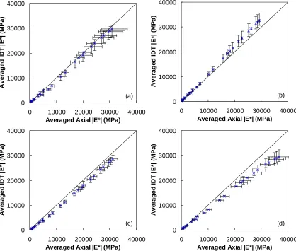
Figure 5.1 Log-log line-of-equality of SA and SI |E*| values for (a) S12.5C, (b) S12.5FE, (c) S12.5CM, and (d) S12.5C-AV-2.

To compensate for this effect, the standard deviation was determined for each frequency. The standard devations from each mixture for a given specimen geometry were averaged. The assumption is a given testing method has a normal variability. Sometimes the

(40)

statistically significant difference exists between the methods. Graphical comparisons are presented to support the statistical results.

0 10000 20000 30000 40000

A ve rag e d I D T | E *| ( M P a) (b) 0 10000 20000 30000 40000

0 10000 20000 30000 40000

A ve raged I D T | E *| ( M P a) (a) 0 10000 20000 30000 40000

0 10000 20000 30000 40000

A ve raged I D T | E *| ( M P a) (c) 0 10000 20000 30000 40000

0 10000 20000 30000 40000

A ve raged I D T | E *| ( M P a) (d)

Figure 5.2 Line-of-equality of SA and SI |E*| values for (a) S12.5C, (b) S12.5FE, (c) S12.5CM, and (d) S12.5C-AV-2.

Figure 5.1 and Figure 5.2 provide evidence that axial compression and IDT

(41)

represent the maximum and minimum |E*| values from these replicates. The number of replicates used is shown in Table 5.1.

5.2.1 Geometry Comparisons

Table 5.2 Statistical Results for Geometry Comparisons Stepdown Bootstrap p-value

Evaluation Comparison Mixture fq1 fq2 fq3 fq4 fq5 fq6 S12.5C 0.60 0.83 0.20 0.81 0.92 0.69 S12.5C-AV+2 0.11 0.32 0.20 0.15 0.070 0.13 S12.5C-AV-2 0.85 0.34 0.066 0.065 0.067 0.041 S12.5C-AC+1 0.55 0.44 0.11 0.15 0.041 0.041 S12.5C-AC-1 0.31 0.31 0.065 0.20 0.13 0.067 S12.5CM 0.16 0.23 0.065 0.20 0.26 0.29 S12.5FE 0.24 0.14 0.27 0.067 0.071 0.18 S12.5F 0.92 0.88 0.27 0.43 0.12 0.18 IDT Procedure SA vs SI

B25.0C 0.028 0.11 0.54 0.92 0.74 0.45 S12.5C 0.92 0.59 0.92 0.15 0.239 0.740 Prism SA vs SP

S12.5FE 0.27 0.80 0.91 0.92 0.92 0.800

Note: * Compaction (first letter): (S)GC or (R)olling Wheel Geometry (second letter): (A)xial, (P)rism, or (I)DT

IDT versus Axial

(42)

testing is suitable for a wide range of mixtures. Measurements with the S12.5CM mixture show statistical insignificance at low reduced frequencies (fq1-fq4). Also of note is the S12.5-AV-2 mixture, where the results show p-values near the 0.05 threshold, except for fq2. A closer analysis of these results suggests that the data from IDT and axial

compression are indeed different. The reason fq2 for S12.5-AV-2 is highly insignificant is the IDT curve crosses the axial curve at this point. This is an undesirable result because it indicates that the shapes of the curves are different. Even though some mixtures show a significant difference, most of the mixtures show insignificance. Based on statistical information, IDT and axial mastercurves are concluded to be similar.

Axial versus Prism

Another geometry comparison of interest is that of axial and prismatic specimens. It is expected that prismatic and axial specimens should be similar because the compaction and loading directions and state of stress are the same as for axial specimens. The only difference is a smaller cross-sectional area in prismatic specimens to apply the load.

The data in Table 5.2 show that comparisons between prism and axial specimens have no statistically significant difference. The variability of prism testing is the smallest of all three geometries. The average variability of the data points is approximately 10% of the averaged |E*| value. Based on this evidence, comparisons between prism and IDT specimens can be considered similar to comparisons between axial and IDT specimens.

RVE

(43)

the difference between axial, IDT, and prism specimens is statistically insignificant for all frequencies except for the previously mentioned small reduced frequency in the SA versus SI comparison. Given the large aggregate size, and the small RVE (≈ 2), this observation provides evidence that the IDT gauge length of 2 inches and the thickness of 1.5 inch are adequate to capture the response of the mixture. Kim et al. (2004) show an increase in the difference between axial and IDT specimens for increasing nominal maximum size of aggregate (NMSA) values, but this study shows a similarity. Caution should be exercised when comparing IDT and axial mastercurves at low reduced frequencies. Large variability occurs in this region. This variability is to be expected because the lower |E*| value corresponds to 35°C, the temperature at which the material is rather soft and the large aggregate would disproportionately affect the deformation over the gauge length (i.e., larger stiffness gradient between constituent phases).

Table 5.3 Statistical Results for RVE and Non-uniform Stress Stepdown Bootstrap p-value

Evaluation Comparison Mixture fq1 fq2 fq3 fq4 fq5 fq6 S12.5C 0.60 0.83 0.20 0.81 0.92 0.69 SA vs SI

B25.0C 0.03 0.11 0.54 0.92 0.74 0.45 S12.5C 0.92 0.59 0.92 0.15 0.23 0.74 RVE

SA vs SP

B25.0C 0.17 0.85 0.92 0.87 0.84 0.57 S12.5-AV+2 0.62 0.88 0.07 0.07 0.07 0.07 Non-uniform

stress RP vs RI _S12.5FE-AV+3 _0.09 _0.04 _0.92 _0.47 _0.14 _0.15

5.2.2 Non-uniform State of Stress

(44)

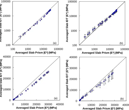
significant difference. In the case of the S12.5C-AV+2 mixture, a nearly significant difference is observed. Significance is seen in the S12.5FE-AV+3 mixture at low reduced frequencies. IDT testing at low reduced frequencies is more variable due to the high strain levels and damage to the specimen at high temperatures. To gain further insight into these observations, Figure 5.3 illustrates the results of the testing in both semi-log and log-log space for the two mixtures.

100 1000 10000 100000

Averaged Slab Prism |E*| (MPa)

A ve raged S la b I D T | E *| ( M P a) (b) 0 10000 20000 30000 40000

0 10000 20000 30000 40000

A ve rage d S lab I D T | E *| ( M P a) (b) 100 1000 10000 100000

100 1000 10000 100000

A ve raged S lab I D T | E *| ( M P a) (a) 0 10000 20000 30000 40000

0 10000 20000 30000 40000

A ve ra g ed S lab I D T | E *| ( M P a) (a)

(45)

In Figure 5.3, for the S12.5C-AV+2 mixture, the RI mastercurve is lower than the RP mastercurve except at the lowest modulus value. For the S12.5FE mixture, the RP and RI mastercurves are similar except in the lower modulus range (i.e., low reduced

frequencies). Once again, the inconsistency in variability for the same geometry is shown, though in this case the RI specimens tend to have larger variability than RP specimens do. Recall that the S12.5C-AV+2 mixture contains cubical aggregates, which research suggests should result in less inherent anisotropy than mixtures with flat and elongated aggregate (Saadeh, 2002). It is, therefore, unexpected that this mixture shows more significance with regard to stress state than the S12.5FE-AV+3 mix, so it is assumed the state of stress does not cause the difference shown. The conclusion is the state of stress does not effect the |E*| values due to the stastical analysis.

5.2.3 Anisotropy

(46)

comparisons from Table 5.3, the challenges of interpreting the data with differences in aging and air voids is observed.

Both compaction and anisotropy comparisons have aging effects and differences in air voids, which are inconsistent. For example, for comparisons of anisotropic effects, each comparison for the S12.5C-AV+2 mixture can be made with the same air voids, but the comparisons for the S12.5FE mixture require data with air voids of 4% (SA) and 7% (RP and RI). In addition, both mixtures contain aging effects due to differences in fabrication. The slab mixture was cooled and reheated instead of immediately proceeding to

compaction like the SGC specimens. The greater aging of the rolling-wheel specimens should produce a higher stiffness. Therefore, the aging effect may account for the smaller distance to the line-of-equality because the S12.5C mixture sat in pans for two months instead of a few days. The difference in aging alone, though, does not explain the reason that the SI and SP mastercurves are higher than those of the RI and RP. Therefore, it should be understood that the following conclusions are drawn with less confidence than if the materials had the same air voids and if there had been no aging effects.

SGC versus Field Compaction

(47)

To compare the effects of compaction on anisotropy, comparisons should be made between the SI and RI. The results in Table 5.4 show the difference in S12.5C is insignificant, but in S12.5FE is significant. It is important to note that the rolling-wheel specimens have higher air voids than the SGC specimens, which could be the source of the difference. But as previously mentioned, air voids showed no statistical difference. Because the effects of compaction based on IDT were inconclusive, a comparison was made with prism specimens (SP vs. RP). This comparison removes any interaction effects from the different states of stress. The results of this comparison show that the difference between mastercurves is significant for the S12.5C. The reason for the difference is the smaller standard deviation used to prism specimens than IDT or axial. If the standard deviation for the IDT testing had been used, the mixture would have no statistical difference.

Table 5.4 Statistical Results for Compaction and Anisotropy Stepdown Bootstrap p-value

Evaluation Comparison Mixture fq1 fq2 fq3 fq4 fq5 fq6 S12.5-AV+2 a 0.17 0.07 0.17 0.27 0.165 0.17 SI vs RI

S12.5FE a 0.20 0.81 0.17 0.04 0.04 0.066 S12.5-AV+2 0.008 0.008 0.008 0.008 0.041 0.065 SGC vs Field

Compaction b

SP vs RP

S12.5FE 0.42 0.66 0.16 0.27 0.42 0.27 S12.5-AV+2 0.11 0.32 0.20 0.15 0.07 0.13 SA vs SI

S12.5FE a 0.24 0.14 0.27 0.07 0.07 0.18 S12.5-AV+2 0.09 0.07 0.21 0.29 0.12 0.12 SA vs RP

S12.5FE a 0.08 0.04 0.19 0.26 0.86 0.88 S12.5-AV+2 0.71 0.18 0.04 0.04 0.03 0.04 Anisotropy b

SA vs RI

S12.5FE a 0.40 0.45 0.27 0.19 0.17 0.19

Note: aair void difference * Compaction (first letter): (S)GC or (R)olling Wheel b

(48)

between the comparisons. The known differences between the two curves, SI and RI, are the method of compaction and the aging. Only the aging condition is inconsistent

between the mix types. As previously mentioned, the effect of aging does not entirely account for the SGC specimens being stiffer than the rolling-wheel specimens. Even though the statistics reveal insignificant influence from the compaction method, a numerical investigation seems to suggest an increase in |E*| values from the SGC. The increase may be a result of the air distribution within a gyratory specimen, since the center of the specimen is known to be denser in the center where the LVDT’s measure deformations than the outside, which could increase the |E*| values. Based on statistics, the values are not different.

Effect of Anisotropy on Field to Laboratory Values

(49)

compaction and stress-strain analysis do not have an effect. In the comparison of SA and RI, a significant difference occurs at high reduced frequencies or at high modulus values. In the S12.5C-AV+2 mixture, the SA values are higher than S12.5C, which is unexpected since S12.5-AV+2 has greater air voids and is less dense, the |E*| values should remain the same or decrease. This difference could explain why S12.5C-AV+2 is different but S12.5FE is not. The results seem to imply that the magnitude of anisotropy is not as great a factor as might be expected. Because the material’s property is measured at low strain levels, which generally does not mobilize the aggregate, this conclusion is reasonable. Results suggest that the compaction direction and stress-strain analysis generally do not have an effect.

5.3 Conclusions

Based on the results presented in this chapter, the following conclusions can be drawn: 1. The statistical difference between IDT and axial specimens is insignificant for a

variety of mixture gradations at low strain levels.

2. Sources of anisotropy and its effects are difficult to isolate. Based on the data, compaction and loading direction have an insignificant effect.

3. Prism specimens provide a good alternative for axial specimens in forensic work. Prisms have statistically similar |E*| values for SGC and rolling-wheel specimens. 4. The effects of non-uniform stress in IDT testing is insignificant compared to

prism specimens.

(50)

test method has a small RVE, which is adequate except at small reduced

frequencies (high temperatures and long loading times), due to the gauge length. 6. The alternative geometries explored in this study appear to reduce the

specimen-to-specimen variability.

Based on these conclusions and the observations in this chapter, the |E*| can be acquired through several geometries with minimal concerns about differences stemming from the RVE, non-uniform states of stress, and anisotropy.

CHAPTER 6 PREDICTING DYNAMIC MODULUS FROM RESILIENT

MODULUS USING AN ARTIFICAL NEURAL NETWORK

6.1 Method

This study has three stages for investigating whether MR data can be used to predict the

|E*| using the ANN: 1) developing a database with corresponding |E*| and MR values; 2)

training the ANN; and 3) verifying the accuracy of the predictions.

Developing a database with |E*| and MR values can be a lengthy task if the properties

are measured in the laboratory, especially for a database comprehensive enough to encompass a large range of mixture variables, such as binders, gradations, NMSA, voids in mineral aggregate, voids filled with asphalt, air voids, etc. The proposed method is to use a comprehensive |E*| database, and then populate the database with MR values using

the method presented.

As previously mentioned, several MR formulations exist. The MR solution used in this

(51)

1 2 (

R

P

M k k

Ud ν

= − ), (6.1)

where

MR = resilient modulus (MPa);

P = applied load (N);

U = recoverable horizontal displacement (m); d = thickness of specimen (m);

ν = Poisson’s ratio; and k1, k2 = (-0.00018, 0.000578).

The unknowns in the equation are the load, the horizontal displacement, and the

Poisson’s ratio. The Poisson’s ratio is assumed to be constant for a given temperature (0.2, 0.35, and 0.45 for 5°, 25°, and 40°C, respectively). To determine the horizontal

displacement amplitude, a two-dimensional viscoelastic formulation is needed to predict a strain history from a given loading history for a biaxial state of the stress. Equation (6.2) shows the formulation for calculating the horizontal strains needed for Equation (6.1). Equation (6.2) is based on the generalized Hooke’s Law in conjunction with the viscoelastic correspondence principle and the plane stress formulations of Hondros (1959):

1 2

0

2( )

( )

t

P

U D t d

ad

γ νγ _τ _τ

π τ

+ ∂

= −

∂

∫

, (6.2)

where

D = compliance

a = loading strip width (m); d = thickness of specimen (m); and

(52)

To predict the horizontal displacement, a representative loading history (i.e. a repeated 0.1 second haversine pulse followed by a 0.9 second rest period) is introduced to Equation (6.2). Once the horizontal strains are calculated, the MR can be calculated by

using Equation(6.1).

After the database has been populated, the next step is to train the ANN. The ANN is a model composed of nonlinear transfer functions, typically a sigmoidal function, between inputs and outputs. The ANN is trained using the feedfoward, backpropagation method. The feedforward portion of the training involves presenting the inputs and the desired outputs (targets) so that the computer program can make the appropriate connections with the transfer functions. The backpropagation portion involves predicting the output using a given input, which is the ultimate purpose of the ANN. The program evaluates the error between the targeted and predicted outputs based on the weighted transfer functions. Using the Levenberg-Marquardt optimization algorithm, the computer selects new weighted values and repeats this process until the program reaches a maximum number of iterations or the minimum error desired. Further information regarding the use of neural networks in pavement applications can be found in Xu et al. (2002).

(53)

the data. If the network has too many degrees of freedom, the data can predict the training data well, but may not be able to interpolate for new inputs, which is the ultimate purpose of training the network.

In order to verify the accuracy of the predictions, an independent database containing both measured |E*| and MR values is used. The measured |E*| values allow for a

comparison between predicted and measured values. The MR data are necessary to

determine if the greater variability in measured MR affects the ANN results.

6.2 Theoretical Background

6.2.1 Determination of Displacements Using the Multiaxial Convolution Integral

For linear elastic materials, the stress-strain relationship is represented by the generalized Hooke’s law. Assume the rectangular coordinate of x1 in the horizontal direction, x2 in

the vertical direction, and x3 in the depth direction of the IDT specimen. Two strains that

are of interest are ε11 and ε22. According to the generalized Hooke’s law, these two strains

are related to stresses as follows:

11 11 22 11 22

1

( ) D( )

E

ε = σ −νσ = σ −νσ ; (6.3)

22 22 11 22 11

1

( ) D( )

E

ε = σ −νσ = σ −νσ , (6.4)

where

E = Young’s modulus and D = compliance.

(54)

11 11 0

( ) [ ( ) ]

t

D t t d

ε τ σ ν τ σ τ

τ 22

∂

= − − −

∂

∫

and (6.5)

22 22 11

0

( ) [ ( ) ]

t

D t t d

ε τ σ ν τ σ τ

τ ∂

= − − −

∂

∫

. (6.6)

The Hondros equations used to calculate the resulting stresses in the horizontal and vertical directions are:

11 2

[ ( ) ( )]

P

f x g x

ad σ

π

= − and (6.7)

22 2

[ ( ) ( )]

P

f x g x

ad σ

π

= − + , (6.8)

where

2 2

2 2 4 4

(1 / ) sin 2 ( )

1 (2 / ) cos 2 /

x R

f x

x R x R

α α −

=

+ + (6.9)

2 2 1

2 2

1 /

( ) tan tan

1 /

x R

g x

x R α

−  − 

= _ _

+

 ; (6.10)

R = radius of specimen (m);

x = horizontal distance from center of specimen (m); and

α = radial angle (radians).

Combining Equations (6.5), (6.6), (6.7), and (6.8) results in the following expressions for the horizontal and vertical strains:

11 1 0 2 ( , ) ( ) {[ ( ) ( )] ( )[ ( ) ( )]} t P

x t D t f x g x t f x g x d

ad ε τ ν τ τ π τ ∂ = − − + − + ∂

∫

; (6.11)

22 2 0 2 ( , ) ( ) {[ ( ) ( )] ( )[ ( ) ( )]} t P

x t D t f x g x t f x g x d

ad ε τ ν τ τ π τ ∂ = − − + + − − ∂

∫

. (6.12)

(55)

11( , )1

l

U ε x t dx

−

=

∫

; (6.13)

22( , )2

l

V ε x t dx

−

=

∫

; (6.14)

or

0 2

( ) [ ( ) ( ) ] ( ) [ ( ) ( )]

t l l

l l

P

U D t f x g x dx t f x g x dx d

ad τ ν τ τ

π τ ₋ ₋

 

∂

= − _ − + − + _

∂  

∫

; (6.15)

0 2

( ) [ ( ) ( )] ( ) [ ( ) ( )]

t l l

l l

P

V D t f x g x dx t g x f x dx d

ad τ ν τ τ

π τ ₋ ₋

 

∂

= − _− + + − − _

∂  

∫

. (6.16)

For the gauge length of 50.8 mm (2.0 in.), Equations (6.15) and (6.16) reduce to:

1 2 0 2 ( ) { ( ) } t P

U D t t d

ad τ γ ν τ γ τ

π τ

∂

= − + −

∂

∫

; (6.17)

1 2 0 2 ( ) { ( ) } t P

V D t t d

ad τ β ν τ β τ

π τ

∂

= − + −

∂

∫

, (6.18)

where the values of β1, β2, γ1, and γ2 are shown in Table 2.1.

Equations (6.17) and (6.18) require two time-dependent material properties, i.e., creep compliance and Poisson’s ratio. It has been proven that the creep compliance of asphalt concrete can be predicted from the |E*| using theoretical relationships (Kim and Lee, 1995). In this study, the approach is used to convert the |E*| mastercurve to the creep compliance is presented in Section 2.1.

The second time-dependent material property in Equation (6.17) is Poisson’s ratio. The time-dependent nature of Poisson’s ratio has been reported in Kim et al. (2004).

(56)

sample-to-sample variability in Poisson’s ratio values. Another difficulty involved in Poisson’s ratio is that Equation (6.17) is difficult to solve because there are two time-dependent properties in the equation. If Poisson’s ratio in Equation (6.17) and (6.18) is assumed to be constant, Equations (6.17) and (6.18) reduce to the following:

1 2

0

2( )

( )

t

P

U D t d

ad

γ νγ _τ _τ

π τ

+ ∂

= −

∂

∫

and (6.19)

1 2

0

2( )

( )

t

P

V D t d

ad

β νβ _τ _τ

π τ

+ ∂

= −

∂

∫

. (6.20)

0.0 0.2 0.4 0.6 0.8

0.0000001 0.0001 0.1 100 100000

Reduced Time (s)

P

o

is

s

ion

's

R

a

ti

o

(ν

)

Replicate 1 Replicate 2

Replicate 4

Replicate 5

Evaluation of Different Methods for Populating the LTPP Materials Database with the Dynamic Modulus

DEDICATION

BIOGRAPHY

ACKNOWLEDGEMENTS

TABLE OF CONTENTS

LIST OF FIGURES

LIST OF TABLES

φ

E'

E''

E*

∑

[ ]

{ } { }

(

)

(

)

∑

∑

∑

φ

σ

ε

(

)

(

)

(

)

(

)

∫

∫

∫

∫

∫

∫

∫

∫

∫

∫

∫

∫

∫

∫

∫

∫

∫