Available Online atwww.ijcsmc.com
International Journal of Computer Science and Mobile Computing
A Monthly Journal of Computer Science and Information Technology
ISSN 2320–088X
IJCSMC, Vol. 4, Issue. 4, April 2015, pg.271 – 285
RESEARCH ARTICLE
Forecasting USD/IQD Future Values
According to Minimum RMSE Rate
ABSTRACT
This paper has used econometric time series to model and forecast the future price of United States Dollar comparing with Iraqi Dinar (USD/IQD) along 2 years, started from 1st January, 2013 to 31st December, 2014. After pre-processing the data to check and fill the missing values using interpolation method, the first effort of this project employs the Auto Regressive Moving Average (ARMA) model, which has been used to prototypical a time series data set. It is establish that the model can be used to suitable the data in the estimation period (2013-2014). 400 ARMA models had been tested in this job. The Root Mean Square Error (RMSE) is used to find best order of the parameter in ARMA model i.e. r, m accurate values.
The forecasting is very important in the analysis of economic and industrial time series, and in sailing and buying movement and investment operation. In order to avoid falling into a financial crisis, the idea in this work is trying to find a model to predict approximately future prices of USD/IQD by predicting three days ahead closing prices based on previous one year closing prices for each three days based on the ARMA model. The proposed model gave close results to actual price when it has been compared to closing prices of year 2014.
Keywords: Time series analysis, USD, IQD, ARMA, RMSE, and Forecastıng.
1. Introduction to Time Series Data Set and Prediction
A time series is a set or structure of detected data arranged in sequential order and in
correspondingly spaced time intervals such as daily or hourly air temperature or prices of
currency values and prices of stock markets. Time series data sets are used in many fields
such as finance and economy, engineering, and science.
Jehan Kadhim Shareef 1
Information System (IS), [email protected] Thi_Qar University/ Media Faculty
Mohammad Abdulrazzaq Thanoon 2
Artificial Intelligent, [email protected]
University of Mosul / Electronics Engineering Faculty
Wijdan Rashid Abdulhussien 3 Soft Computing, [email protected]
The data set has a stationary state if and only if the mean, variance, and autocorrelation of a
univariate time series are not changing over the time. There are many analysis methods apply
to only stationary data sets, and there are several methods to convert a data set to a stationary
such as: transforming it to difference data, or removing the slope from the data set. In order to
forecast future information using specific analysis methods, the researchers rely on historical
data of time series data sets [1].
Currency crisis is a state in which the rate of a currency becomes unstable, production it
difficult for the currency to be used as a dependable medium of exchange. The effect of a
currency crisis can be mitigated by sufficient foreign reserves. Also, it is mention as a type of
financial crisis. So, we tried to program a model able to predict future financial prices like
USD/IQD prices.
There are various statistical analysis methods to process a time series data set. They can be
applied to estimate the future level (estimated value), the trend of observations, or the
variability of the estimation and observations. As an example, time series regression is used
to find out the estimated value of time series data, the trend of the data set, and also the
confidence level of the estimated value. More advanced statistical linear estimation methods
such as Auto-Regressive Moving-Average (ARMA) were developed since many years ago,
and they are still in use for accurate estimations [2].
The ARMA model is a statistical time series analysis technique based on discrete time
dynamic modelling of the observations by using the weighted sum of previous r observations
to predict the expected next observation, building an autoregressive model. Moreover, the
expectation error is considered to represent the external effects to the dynamics of this
autoregressive model, and the weighted average of m of past error terms is used to drive the
model parallel to the observations. The weighted sum of the past observations builds the Auto
Regressive model, and, the weighted average of errors is called the Moving Average part of
ARMA [3].
ARMA model is frequently used as a prediction model [3] [4] [5] [6] [7] [8] [9] [10]. It gives
the researchers the prospect to forecast the future value of time series data set. J., A., M. and
and the result has been proven that the ARMA model is work well for forecasting the future
values, especially in the longer-term forecasting.
2. Procedures and Material of this Work
2.1 Theoretical Background for ARMA
The Auto-Regressive–Moving-Average (ARMA) model for prediction of the future value of
a time series data set was proposed by Peter Whittle in 1951 [9], and more developed by
George E. P. Box and Gwilym Jenkins in 1971 [10]. ARMA model comprises two
polynomial parts, one contains the past values of the target variable in an auto regressive
structure (AR), and the other one contains the moving average of the prediction error as an
input variable (MA). The notation AR(r) refers to the autoregressive model of order r. It is
written: t i t r i i
t
c
x
x
1
(2.1)
where are weighting parameters for autoregressive model, c is a constant, and the random
variable is white noise.
The notation MA(m) refers to the moving average model of order m. It is set up by taking the
average of sub orders. It is written:
i t m i i t t
x
1 (2.2)where the θ1... θm are the parameters of the model, is the expectation of (often assumed
to equal 0), and the , are again, white noise error terms.
The notation ARMA(r,m) refers to the model with r autoregressive terms and m
moving-average terms: i t m i i i t r i i t t
x
x
1 1 (2.3)The collective model, ARMA(r,m) provides two benefits; the autoregressive part (AR)
part (MA) predicts the effect of disturbances which appears as error in the auto regressive
model.
2.2 The Data Sets of USD/ IQD Price
In this work, the three-day-ahead prediction of USD/IQD required time series daily closing
prices for the period starting from 1st January, 2013 to 31st December, 2014, for total 2
years. The data is collected from the financial data accessible on
www.oanda.com/currency/historical-rates/ [11].
Missing vectors and values are an important problem in time series data sets when they are
used for forecasting purposes, because the missing part misleads the features of the time
series (Missing vector means no data available for a day, and missing value means that some
of the values of a daily record are missing) [12]. Mathematically, there are methods to
construct missing data vectors within the range of a discrete data set, such as using previous
day or next day values to complete the missing days. A commonly used method to fix
missing data is method of linear interpolation, i.e. to complete missing values using the
weighted average of the previous and next day values.
Linear interpolation finds the target y for a value of x using the previous (xa, ya) and the next
(xb, yb) values as given by equation 3.1 [13].
)
(
)
(
)
(
a b
a a
b a
x
x
x
x
y
y
y
y
Figure 2.1: Daily Original Price (USD/IQD)
Figure 2.1 shows daily closing price of USD comparing with IQD values with minimum
value = 1123 IQD, maximum value = 1180 IQD, mean= 1150 IQD, and stander division
(Std) = 9.081 IQD. The random movement of the prices is clearly visible in the plot, where
the prices of 1 USD was 1144 IQD at the start of the year 2013, makes a sharp bottom down
to 1123 IQD after five months in the same year, design the financial crisis, and recovers
slowly in the forward months back to the 1144 IQD level and more. The plot of the prices in
long period clears that the prices are non-stationary.
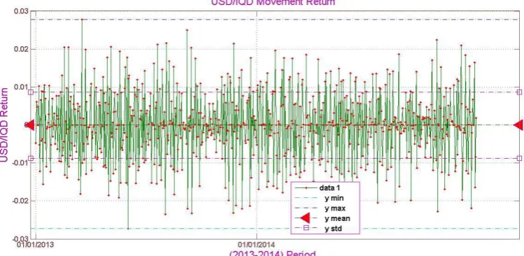
The return value of the USD/IQD for the period (2013-2014) is shown in Figure 2.2, where
the mountaintops of return take place especially when the prices start to increase or decrease.
The largest positive return= 0.0276 and negative return= -0.0272 which were happened at
2013. As recognized in the figure 2.2, the return values have zero mean over the long period,
Figure 2.2: USD/IQD Original Return
2.3 Parameter Estimation and Performance Criteria
The target of forecasting in this test is to predict the three-days-ahead return values xˆk+3
correctly. The performance of the ARMA model is measured by the smallness of the error of
prediction, comparing the predicted value xˆk+3 by the actual return of three-days-later, i.e.,
ek= xk+3 - xˆk+3. During the estimation of values for a long period of time, the error may
change in positive and negative directions, and their sum i ek-i might stay nearly zero
although the magnitude of error is much higher than the sum of errors. Therefore i ek-i is not
a performance measure for the predicted values by an ARMA model. In the most systems and
small errors are tolerated to a degree, however, large errors are intolerable because they may
result in unexpected hazards. Squaring the error, ek-i, makes it positive, and also increases the
effect of larger errors nonlinearly as desired in many cases. The mean of squared errors needs
square rooted to make it compatible to the output. The resulting performance measure for n
successive days of predictions using an ARMA model is:
eRMSE=
n
i en i
n 1 2
1
1
(2.5)
It is called root-mean-square-error, and commonly used in estimation as a performance
metrics [14]. The parameters of an ARMA(r, m) model may be trimmed to reduce eRMSE of
predicted return.
For practical considerations, ARMA model shall have the smallest order, which provides an
MA, are structural parameters of ARMA model, and in the literature, there are methods based
on plotting the partial autocorrelation functions for an estimate of r, and m [15].
2.4 The
r
and
m
Values
by Autocorrelation and Partial Autocorrelation
The autocorrelation function (ACF) measures the similarities of a series starting from xt
against another series starting from xt-h. It is used for predictions. An auto correlated time
series is predictable, probabilistically, because upcoming values rely upon present and
previous values. The time series plot could be a tool for measurement the autocorrelation of a
time series. Positive autocorrelation may show up a plot as remarkably long runs of many
consecutive observations higher than or below the mean. Negative autocorrelation may show
up as a nosily low incidence of such runs. For computing autocorrelation the relative a
horizontal line planned at the sample mean is helpful in evaluating autocorrelation with the
time series plot.
In addition, a partial autocorrelation (PACF) is defined to give the correlation between xt and
xt-h after intermediate correlation has been removed. The PACF is obtained from the set of
difference equations related to the ACF. Equation 2.6 shows the formula for the sample lag-h
autocorrelation. For an observed series x1, x2,...,xT and the sample meanx, the sample lag-h
autocorrelation is given by [15] [16]:
lag-h
T t t T ht t t h
x x x x x x 1 2 1 (2.6)
Figure 2.3 and Figure 2.4 show the lag-h autocorrelation (ACF) and lag-h partial
autocorrelation (PACF) for USD/IQD Movement at period (2013-2014).
For data set analysis such USD/IQD price, it is difficult to identify the patterns for AR and
MA models directly. For AR(r) model, the partial autocorrelation (PACF) will be close to
zero at lags greater than r. For a MA (m) model the autocorrelation (ACF) be close to zero at
lags greater than m. As a result, the expected m values according to ACF were 10, 11, 13 and
19 (Figure 2.3), and the r values agreeing to PACF were 8, 10, and15 in USD/IQD price data
Figure 2.3: Autocorrelation of USD/IQD Movement
In figure 2.3 and 2.4, x-axis represents the order of m in ACF and order of r in PACF, y-axis
represents the lag-h of ACF and PACF for the time series data set.
2.5 Finest
r, m
Values of ARMA Model
The parameters r and m are called structural parameters to distinguish them from the autoregressive parameters i and moving average parameters i in the ARMA (r, m). The best
forecasting ARMA (r, m) model is obtained by two steps which are the r and m values that
give the lowest estimation error (RMSE) of three days ahead forecasting over the previous
one year data set. The crucial goal of the forecasting is to have sufficiently small error of
prediction with less structural order so that satisfactorily accurate prediction is obtained by an
ARMA model with the minimum possible order.
For example in the partial auto correlation function (Figure 2.4), the 8th, 10th, and 15th terms (including them as zero-term+Lag) have significant high values. The RMSE values for
USD/IQD indicates clearly minimums at (r, m)=(3.3), (3,9), (6,6), (8,9), (10,10), (9,12), and
(15,15).
Principally, the preferred model is the model which has a minimum number of parameters to
escape the large number of computational steps as much as possible, eliminate increase the
percentage of error and become close to the prediction precision. In this work, the minimum
RMSE value = 0.00003 corresponding to ARMA (10, 10) model, rather than RMSE value
with ARMA (3, 3) and ARMA (6, 9) were 0.00006 and 0.00009 respectively. So, the data set
fitted by ARMA (10, 10) model to get the precision expecting future data set. Figure 2.5
Figure 2.5: Block diagram the project
3. Results and Discussion
3.1 Forecasting
Guess of the future using the movement and forms in a set of past available observations
Time series data set (closing price of USD/IQD from 1/1/2013 to
31/12/2014)
Start
Pre-processing missing values calculation
Data partitioning for each day (closing prices of previous one
year)
Search best ARMA(r, m) model among 400 models according to RMSE value
Fitting closing price by the best ARMA(r, m) model
Forecasting the future closing price of USD/IQD
resources for a future period of time. The forecasting of economic and industrial time series is
important as a tool of analysis for the business decisions such as selling or buying, and hold
transactions in the markets [17] [18]. As a methodical technique, predicting helps
organizations and companies for decision making in the state of uncertainty.
For the idea of this work, the objective period lies on the years from 2013, to 2014. The
observations are collected as the time series of closing prices for the USD/IQD price which is
suitable by an ARMA model.
The h-day-ahead prediction error is ek,h = xk+h - xˆk+h, where xk+h is the actual return value at
the end of h-day and xˆk+h is the forecasted return value by ARMA model.
3.2 The Results of Forecasting Using ARMA Model
In this idea, the forecasting of three-days-ahead return is gains by training the
ARMA (10, 10) model for each predicted day by using its previous one year of USD/IQD
price. Once the estimation errors et-i is calculated from the previous actual values and their
estimated by et-i= xt-i - xˆt-i, the future values
e
ˆ
xt is predicted by ARMA (10, 10) modelwith an error et. Figure (3.1) shows the original and forecasting prices along 2014 on one
graph.
X-axis represented to the period from 1/1/2013 to 31/12/2014 and y-axis denotes USD/IQD
price. The forecasting process happening from 1/1/2014 because each three days are
Figure (3.1): The Original and Predicted USD/IQD Price
The error means a difference between original and predicted price. For instance, in (6/1/2014)=3.85, i.e. (1146.4- 1142.55), the table 3.1 below contain sample of the actual and prediction price of USD/IQD by ARMA (10, 10) model.
Table 3.1: Actual and predicting USD/IQD closing price
Date Original price Forecasting Price by ARMA(10,10)
6/1/2014 1146.4 1142.55
7/1/2014 1154.88 1157.88
8/1/2014 1168.11 1169.11
9/1/2014 1168.11 1171.11
10/1/2014 1168.11 1166.11
11/1/2014 1153.88 1154.88
12/1/2014 1165.5 1164.5
13/01/2014 1165.5 1163.5
14/01/2014 1165.74 1164.19
15/01/2014 1164.66 1162.55
16/01/2014 1152.98 1150.88
17/01/2014 1152.98 1152.1
18/01/2014 1166 1164.7
19/01/2014 1147.1 1145.9
20/01/2014 1162.8 1161.6
21/01/2014 1145.68 1147.18
22/01/2014 1150.09 1151.59
23/01/2014 1146.91 1143.81
24/01/2014 1150.32 1150.68
25/01/2014 1147.07 1149.47
28/01/2014 1155.04 1154.16
29/01/2014 1165.29 1166.69
30/01/2014 1146.74 1148.04
31/01/2014 1144.24 1142.91
1/2/2014 1154.31 1151.31
2/2/2014 1177.2 1173.9
3/2/2014 1177.22 1178.72
4/2/2014 1167.84 1168.07
5/2/2014 1148.47 1150.13
6/2/2014 1146.05 1148.05
7/2/2014 1147.14 1145.94
8/2/2014 1147.57 1145.07
9/2/2014 1133.5 1137.5
10/2/2014 1133.5 1135.27
11/2/2014 1144.78 1143.28
12/2/2014 1150.49 1147.99
13/02/2014 1167.21 1164.11
14/02/2014 1146.7 1143.6
15/02/2014 1152.85 1149.75
16/02/2014 1173.4 1170.3
17/02/2014 1163.8 1160.7
18/02/2014 1172.49 1169.39
19/02/2014 1163.75 1159.65
4. Conclusions
This paper has practical Auto-Regressive Moving Average (ARMA) model on the indexes of
USD/IQD time series data set from 2013 to 2014 with the intention to predict the closing
price and the possibility for the companies to make a decision of selling or buying operations.
The greatest structural parameter set (r, m) of ARMA(r,m) model is investigated among 400
cases: {ARMA(1,1), ... ARMA(20,20)} were obtained by pointed the minimum RMSE case.
The ARMA (10,10) model was used to fitting USD/IQD price to get future price because it
was record a minimum value of RMSE among 400 tested model (RMSE= 0.00003).
Bibliography
[1] R. P. Schumaker and H. Chen, "Textual Analysis of Stock Market Prediction Using Financial News Articles," in Americas Conference on Information Systems, Arizona, 2006.
[2] S. Fallaw, "Modeling long -run bahavior with the fractional ARIMA model," Monetary Economics, no.
29, pp. 227-302, 1992.
[3] P. J. Brockwell and R. A. Davis, Time Series: Theory and Methods, 2nd ed., Colorado State University,
1991.
[4] L. T. J., G. A. , . D. B. M. and . D. F. A., "Forecast of hourly average wind speed with ARMA models in
Navarre (Spain)," Solar Energy, vol. 79, p. 65–77, 2005.
[5] A. G. Paul , "The Time-Series Behavior of Quarterly Earnings: Preliminary Evidence," Journal of
Accounting Research, vol. 15, no. 1, pp. 71-83, 1977.
[6] . P. Ping-Feng and L. Chih-Sheng , "AhybridARIMAand support vector machines model in stock price
forecasting," Omega , no. 33, p. 497 – 505, 2005.
[7] . L. S. Brian, M. . W. Billy and K. . O. R. , "Comparison of parametric and nonparametric models for
traffic flow forecasting," Transportation Research Part C, no. 10, p. 303–321, 2002.
[8] J. N. Francisco , C. Javier , J. . C. Antonio and . E. Rosario, "Forecasting Next-Day Electricity Prices
by Time Series Models," IEEE TRANSACTIONS ON POWER SYSTEMS, vol. 17, no. 2, pp. 342-348,
2002.
[9] P. Whittle, Hypothesis Testing in Time Series Analysis, 1st ed., English Universities Press, 1951.
[10] E. P. George, M. J. Gwilym and C. R. Gregory, Time Series Analysis: Forecasting and Control,
[11] "OANDA," 3 3 2015. [Online]. Available: www.oanda.com/currency/historical-rates/.
[12] J. L. Roderick and B. R. Donald, Statistical Analysis with Missing Data, New Jersey: John wiley
&sons,Inc., 2002.
[13] B. Thierry , . T. Philippe and U. Michael , "Linear Interpolation Revitalized," IEEE TRANSACTIONS
ON IMAGE PROCESSING, vol. 13, no. 5, pp. 710-719, 2004.
[14] J. W. Cort and M. Kenji , "Advantages of the mean absolute error (MAE) over," Clim Res, vol. 30, pp.
79-82, 19 December 2005.
[15] C. Javier , E. Rosario , J. N. Francisco and J. C. Antonio , "ARIMA Models to Predict Next-Day
Electricity Prices," IEEE TRANSACTIONS ON POWER SYSTEMS, vol. 18, no. 3, pp. 1014-1020,
AUGUST 2003.
[16] A. G. Paul , "The Time-Series Behavior of Quarterly Earnings: Preliminary Evidence," Journal of
Accounting Research, vol. 15, no. 1, pp. 71-83, 1977.
[17] B. V. Nagendra and C. Dr. Tansen , "FORECASTING ECONOMIC TIME SERIES DATA USING
ARMA," pp. 1-8.
[18]
J. C. Antonio , A. P. Miguel , E. Rosa and . B. M. Ana, "Day-Ahead Electricity Price Forecasting Using
the Wavelet Transform and ARIMA Models," IEEE TRANSACTIONS ON POWER SYSTEMS, vol. 20,