Communication
1
A probability density function generator based on
2
deep learning
3
Chi-Hua Chen 1, Fangying Song 1,*, Feng-Jang Hwang 2 and Ling Wu 1
4
1 College of Mathematics and Computer Science, Fuzhou University, China; [email protected];
5
[email protected]; [email protected]
6
2 School of Mathematical and Physical Sciences, University of Technology Sydney, Australia;
Feng-7
8
* Correspondence: [email protected]; Tel.: +86-19959346509
9
10
Abstract: To generate a probability density function (PDF) for fitting probability distributions of
11
real data, this study proposes a deep learning method which consists of two stages: (1) a training
12
stage for estimating the cumulative distribution function (CDF) and (2) a performing stage for
13
predicting the corresponding PDF. The CDFs of common probability distributions can be adopted
14
as activation functions in the hidden layers of the proposed deep learning model for learning actual
15
cumulative probabilities, and the differential equation of trained deep learning model can be used
16
to estimate the PDF. To evaluate the proposed method, numerical experiments with single and
17
mixed distributions are performed. The experimental results show that the values of both CDF and
18
PDF can be precisely estimated by the proposed method.
19
Keywords: probability density function; cumulative distribution function; deep learning
20
21
1. Introduction
22
To explain trends or phenomena, statistic tools and probability models are usually applied to
23
analyse real data. Various common probability distributions (e.g. exponential distribution (ED),
24
normal distribution (ND), log-normal distribution (LD), gamma distribution (GD), etc.) are used as
25
the assumptions about the distribution of practical data [1]. The CDF and PDF of real data, however,
26
could be complex and irregular, so serious errors would be incurred by the naive assumptions. This
27
study proposes a deep learning method [2] that develops a neural network to learn the CDF of real
28
data and fit the corresponding PDF.
29
2. Method
30
The proposed deep learning method is comprised of two stages: (1) a training stage for
31
estimating the CDF and (2) a performing stage for predicting the corresponding PDF (shown in
32
Figure 1).
33
In the training stage, practical data can be collected and analysed for generating actual
34
cumulative probabilities. A deep learning model retaining multiple layers (i.e. an input layer, hidden
35
layers and an output layer) is constructed to learn a CDF in accordance with the actual cumulative
36
probabilities (shown in Figure 2). The input layer includes the random variable x, the actual CDF of
37
which is denoted by F, and the output layer contains the estimated CDF of x, denoted by F. The
38
CDFs of common probability distributions can be adopted as the activation functions in the hidden
39
layers. For example, the CDFs of ED, ND, LD, and GD [1] (denoted by f1, f2, f3, and f4, respectively)
40
can be used as the activation functions (shown respectively in Eq. (1), (2), (3), and (4), where ,
1
,
41
1 s
,
2
, s2, , and are all parameters). In Eq. (4),
, ,x
is the lower incomplete gamma42
function, and
is the gamma function. Furthermore, the number of neurons with different43
activation functions can be extended to n, and the CDF can be estimated by Eq. (5) in accordance with
44
a weight set (i.e.
w w1, 2,...,wn
). The loss function of the proposed deep learning model is defined by45
Eq. (6) according to the estimated CDF (i.e. F ) and the actual CDF (i.e. F) for minimising the
46
estimation error. The gradient descent method is applied to the setting of parameters. The partial
47
differential of E with respect to each parameter is calculated (Eq. (7)-(14)), and the parameter in the
48
(k+1)-th iteration can be updated in accordance with the aforementioned partial differential in the
k-49
th iteration (Eq. (15)-(22), where η is the learning rate). In Eq. (13), ( ) is the digamma function. The
50
number of hidden layers can be increased to estimate a relatively complex CDF.
51
52
Figure 1. The proposed deep learning method for estimating practical probability distributions.
53
54
Figure 2. The structure of the proposed deep learning model.
55
56
1
1
x
f
e
(1)
1 2
1
1
1 erf
2
2
x
f
s
(2)
2 32
ln
1
1 erf
2
2
x
f
s
(3)
Actual Cumulative Probabilities
Deep Learning Model Training Stage
Estimated CDF
Differential Deep Learning Model Performing Stage
Estimated PDF
x
4
, ,
x
f
(4)
1 1 n i i i n i iw f
F
w
(5)
2 21
1
2
2
E
F
F
(6)
1 2 1 ni j i
i
n
j j
i i
w f
f
E
E
F
w
F w
w
(7)
1 1 1 1 x n i if
E
E
F
w
xe
f
F
w
(8)
1
2 2 1 2 2 2 2 21 1 1
1
1
2
x s n i if
E
E
F
w
e
f
F
s
w
(9)
1
22 1 1 2 2 2 2
1 2 1 1
1
2
x s n i ix
f
E
E
F
w
e
f
s
F
s
s
w
(10)
22 2 2 ln 3 3 2 2 3
2 2 2
1
1
2
x s n i if
E
E
F
w
e
f
F
s
w
(11)
22 2 2 ln 2 3 3 2 2
2 3 2 2
1
ln
2
x s n i ix
f
E
E
F
w
e
f
s
F
s
s
w
4 4 4 0 0 11
ln
1
1
l l x x n l l i if
E
E
F
f
F
x
x
l
w
x
x
x
e
e
l
l
w
(13)
4 4 4 11
x n i if
E
E
F
w
x
e
f
F
w
(14)
( )
1 k
k k
j j k
j
E
w
w
w
(15)
1 k k k kE
(16)
1 1 1 1 k k k kE
(17) 1 1 1 1 k k k kE
s
s
s
(18)
1 2 2 2 k k k kE
(19) 1 2 2 2 k k k kE
s
s
s
(20)
1 k k k kE
(21)
1 k k k kE
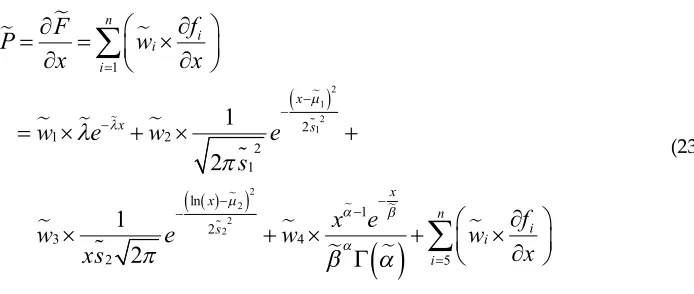
(22)In the performing stage, the differential equation of trained deep learning model described by
57
Equation (23) is derived to obtain the estimated PDF (i.e. P).
2 1 2 1
2 2 2 2
1
2 1 2
2 1 ln
1 2
3 4
2 5
1
2
1
2
ni i i
x
x s
x x
n
i s
i i
f
F
P
w
x
x
w
e
w
e
s
f
x
e
w
e
w
w
x
xs
(23)
3. Experimental Results and Discussions
59
In the numerical experiments, single and mixed common probability distributions with the
60
number of records denoted by m were designed, and the proposed method was evaluated in terms
61
of the mean absolute percentage errors (MAPEs). The MAPE of the estimated CDF (i.e.
F
M ) is defined
62
as Eq. (24) according to F and F, and the MAPE of the estimated PDF (i.e. MP) is defined as Eq. (25)
63
according to P and P.
64
1
100%
m k
k
F
k k
F
F
M
F
m
(24)
1
100%
m k
k
P
k k
P
P
M
P
m
(25)Six test cases, including single ED, single ND, single LD, single GD, and two mixed distributions
65
(MDs) of single ND and single GD with different parameters, were set in the experiments, where the
66
proposed deep learning model for comparison was constructed with f1, f2, f3, and f4. The simulated
67
experimental results are shown in Tables 1, 2, 3, and 4.
68
69
Table 1. MAPEs of the estimated CDF with single distributions.
70
m Case 1: ED
(=0.5)
Case 2: ND (=1,=0.5)
Case 3: LD (=1,=0.5)
Case 4: GD (=0.1,=0.5)
2 0% 0% 0% 1.29%
5 0% 0% 0% 0.20%
40 0% 0% 0% 0%
71
Table 2. MAPEs of the estimated PDF with single distributions.
72
m Case 1: ED
(=0.5)
Case 2: ND (=1,=0.5)
Case 3: LD (=1,=0.5)
Case 4: GD (=0.1,=0.5)
2 0% 0% 0% 9.30%
5 0% 0% 0% 1.58%
40 0% 0% 0% 0.01%
Table 3. MAPEs of the estimated CDF with mixed distributions.
74
m Case 5: ND + GD
(=1,=0.5,=0.1,=0.5)
Case 6: ND + GD (=1,=0.5,=2,=10)
2 5.12% 22.77%
5 2.20% 6.60%
40 0.01% 0.01%
75
Table 4. MAPEs of the estimated PDF with mixed distributions.
76
m Case 5: ND + GD
(=1,=0.5,=0.1,=0.5)
Case 6: ND + GD (=1,=0.5,=2,=10)
2 31.41% 16.70%
5 16.04% 19.10%
40 1.39% 0.09%
77
In Case 1, a single ED with the parameter
=0.5
was used as the benchmark, and different78
numbers of records (i.e. m=2, 5, and 40) were considered to analyse the MAPEs of the estimated CDF
79
and PDF. Both MF and MP are 0%, so the proposed method can obtain a precise estimated PDF for
80
Case 1. In Cases 2 and 3, a single ND with
( , ) (1,0.5)
and a single LD with the same parameters81
were generated, respectively. The PDF was precisely estimated again by the proposed method for
82
both cases. In Case 4, a single GD with
( , ) (1,0.5)
was set to train and test the proposed deep83
learning model. The experimental results show that the estimated CDF and PDF with MAPEs no
84
more than 0.01% can be obtained for m40 even though the GD is a relatively complex probability
85
distribution.
86
As for the analyses of MDs, Cases 5 and 6 were designed to combine single ND and single GD,
87
and the MAPEs of the corresponding estimated CDFs and PDFs were provided in Tables 3 and 4. In
88
Case 5, the parameters
( , , , ) (1,0.5,0.1,0.5)
were adopted to generate an MD. The MAPE of89
the estimated PDF can be less than 1.4% when
m
40
. In Case 6, a relatively complex MD was90
generated with the parameters
( , , , ) (1,0.5,2,10)
. The proposed method can precisely91
estimate the CDF and PDF with MAPEs no more than 0.01% and 0.09%, respectively, for
m
40
.92
4. Conclusion and Future Work
93
This study proposes a deep learning method to learn the potentially complex and irregular
94
probability distributions, and the differential equation of trained deep learning model can be used to
95
estimate the corresponding PDF. The experimental results demonstrate that the proposed method
96
can precisely estimate the CDFs and PDFs for single and mixed probability distributions. Future
97
research could be conducted by assessing the proposed model with real data. Moreover, the accurate
98
CDF and PDF of real-data probability distribution can be produced to improve further analyses with
99
game theory or queueing theory.
100
Author Contributions: conceptualization, Chi-Hua Chen and Fangying Song; methodology, Chi-Hua Chen and
101
Fangying Song, Feng-Jang Hwang; software, Chi-Hua Chen and Fangying Song; validation, Chi-Hua Chen and
102
Fangying Song; formal analysis, Chi-Hua Chen and Fangying Song; investigation, Chi-Hua Chen and Fangying
103
Song; resources, Chi-Hua Chen and Fangying Song; data curation, Chi-Hua Chen and Fangying Song; writing—
104
original draft preparation, Chi-Hua Chen and Fangying Song; writing—review and editing, Fangying Song and
105
Ling Wu.
106
References
108
1. King, M.: ‘Probability density function’ in King, M. (Ed.): ‘Statistics for process control engineers: a practical
109
approach’, John Wiley & Sons Ltd., New York, 2017.

![External trade monthly statistics [Monthly external trade bulletin] 6 7/1986/Commerce exterieur statistiques mensuelles [bulletin mensuel du commerce exterieur] 1986 6 7](data:image/gif;base64,R0lGODlhAQABAIAAAP///wAAACH5BAEAAAAALAAAAAABAAEAAAICRAEAOw==)