Symbolic Side-Channel Analysis for Probabilistic Programs
Pasquale Malacaria∗, MHR. Khouzani∗, Corina S. P˘as˘areanu†, Quoc-Sang Phan‡, Kasper Luckow† ∗Queen Mary University of London, London E1 4FZ, UK
†Carnegie Mellon University, PA 15213, and NASA Ames Research Center, Moffett Field, CA 94035, USA ‡Fujitsu Laboratories of America, Sunnyvale, CA 94085, USA
Abstract—In this paper we describe symbolic side-channel analysis techniques for detecting and quantifying information leakage, given in terms of Shannon and min-entropy. Measur-ing the precise leakage is challengMeasur-ing due to the randomness and noise often present in program executions and side-channel observations. We account for this noise by introducing additional (symbolic) program inputs which are interpreted probabilistically, using symbolic execution with parametrized model counting. We also explore a sampling approach for increased scalability. In contrast to typical Monte Carlo tech-niques, our approach works by sampling symbolic paths, repre-senting multiple concrete paths, and uses pruning to accelerate computation and guarantee convergence to the optimal results. A key novelty of our approach is to provide bounds on the leakage that are provably under- and over-approximating the exact leakage. We implemented the techniques in the Symbolic PathFinder tool and demonstrate them on Java programs.
1. Introduction
Pervasive proliferation of computer systems has in-creased access to sensitive information, ranging from finan-cial and medical records of individuals to trade and military secrets of corporations or countries. It has become critical to develop tools and techniques to ensure that software systems that manipulate sensitive data do so in a secure manner. The confidentiality of secret data is particularly hard to achieve if an attacker can observe non-functional characteristics of a program behavior, for instance by measuring execution times or memory usage. Side-channel attacks [7], [8], [20], [24] aim to recover secret program data based on this kind of observations. Side-channel attacks are of grave concern and they have been shown to pose serious security threats. For instance, they can recover cryptographic keys from well-known encryption/decryption algorithms [7] or derive user-sensitive data from common compression algorithms [20].
In this paper we describe symbolic analysis techniques for quantifying information leaks in side channels. A key obstacle in reasoning about side-channel attacks is the randomness and noise that are often present in program executions and side-channel measurements. This can come from “outside” the program, due to measurements made on noisy hardware platforms or over busy networks, but can also come from “inside” the program, due to explicit
calls toRandommethods in implementations of randomized algorithms (that are often used in security applications), or due to the thread scheduler or the garbage collector, which behave non-deterministically. Furthermore randomness can be introduced as a countermeasure against attacks, e.g. by adding random delays to a program to make it difficult for an adversary to infer secrets based on timing measurements. Thus, it is important to develop precise side channel analysis techniques to assess program leakage in the presence of ran-dom or noisy behavior and to determine if the implemented countermeasures are indeed effective.
To address this problem, we model both internal and external noise by creating additional (symbolic) inputs to the program. Conditions on these inputs are interpreted probabilisticallyusing a probabilistic extension to symbolic execution [16]–[18]. The technique uses model counting over constraints collected with symbolic execution to com-pute probabilities of different program paths. In this paper, we adapt the technique to computing Shannon and min-entropy leakage in the presence of internal and external randomness (or noise). We further describe optimizations based on symbolic projection [1] to avoid explicit enu-meration over secret values. Our analysis is parametrized by an observation model which allows us to obtain the side-channel measurements from the execution of program instructions.
To address the potential scalability issues associated with symbolic execution and model counting, we also explore partial exploration techniques that sample the symbolic pro-gram space to gradually collect symbolic paths. In contrast to typical Monte Carlo approaches, the techniques sample over the symbolic paths which represent multiple concrete paths. Furthermore, each symbolic path needs to be sam-pled only once and is subsequently pruned, accelerating the analysis. Our key contribution is to provide concrete (non-probabilistic) lowerandupper boundson the informa-tion leakage, for min-entropy and Shannon-Entropy leakage, based on the partial exploration analysis. The computed bounds hold for any partial exploration (hence they are “any-time”), improve with more symbolic samples and are guaranteed to converge to the exact value of leakage.
There are few existing tools that can cope with noisy ob-servations. Statistical analysis tools, such as LeakWatch [9], are often imprecise and require a huge number of samples. These tools run the program multiple times and use the
c
outcome of each execution to get an estimate of the in-formation channel (joint probabilities) and any function of it, specifically, leakage values. In contrast to our symbolic approach, statistical approaches have the advantage that they can be used in a “black-box” fashion, where no knowledge of the program or noise distribution is assumed. However, due to the random nature of sampling, the leakage values provided by statistical approaches are only approximate, with no guarantee that they over- or under- approximate the real leakage, which may lead to many false results (positive or negative). Furthermore the accuracy measures such as the confidence intervals provided by e.g. LeakWatch are still probabilistic, and to get a reliable value for them one often needs a large amount of samples. In contrast, our symbolic analysis technique is exact and our estimation approach reports bounds that are provably under- and over-estimating the real leakage, while avoiding resampling of the same (symbolic) path.
We have implemented the exact and partial symbolic analyses in the Symbolic PathFinder tool [38]. We illustrate them in the context of Java applications where we show how to obtain tight bounds on the leakage in the presence of internal and/or external randomness. Our approach can be easily adapted to work with other symbolic execution tools, targeting other programming languages.
Contributions and roadmap.
The main contributions of this work are:
• Introducing a symbolic execution framework for the analysis of side channels in probabilistic programs (Sections 4 and 5);
• Combining this symbolic execution analysis with Barvinok parametrized model counting to optimize the computation (Section 6);
• Developing a symbolic sampling approach to scale up
the computation, and proving guarantees in terms of converging concrete upper and lower bounds, both for Shannon and min-entropy leakage, for our symbolic sampling algorithms (Section 7);
• Demonstrating the applicability of these techniques
to challenging programs (provided by DARPA) and exhibiting the merits of our techniques compared with tools that use standard Monte Carlo techniques; we use “Leakwatch” [9] for comparison (Section 8).
2. Motivating Example
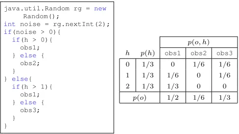
We illustrate our analysis with the example in Figure 1. Assume that the sensitive data h is uniformly distributed over the domainD={0,1,2}, that is:
p(h= 0) =p(h= 1) =p(h= 2) = 1 3
The observableo, which can be for instance the execution time or the runtime power consumption, has three dis-tinct valuesobs1,obs2, andobs3. The instance method
java.util.Random rg = new Random();
int noise = rg.nextInt(2); if(noise > 0){
if(h > 0){ obs1; } else {
obs2; } } else{
if(h > 1){ obs1; } else {
obs3; } }
p(o, h) h p(h) obs1 obs2 obs3
0 1/3 0 1/6 1/6 1 1/3 1/6 0 1/6 2 1/3 1/3 0 0
p(o) 1/2 1/6 1/3
Figure 1: An example Java program and its corresponding joint probability matrix for(h, o).
nextInt(2)ofjava.util.Randomalso returns a uni-formly distributed value from the set{0,1}, and thus:
p(noise >0) =p(¬(noise >0)) = 1 2.
From the probability distribution of h andnoise, con-structing the joint probability matrix for(h, o)as in Figure 1 is straightforward. For example(h= 0, o=obs1)cannot happen, so its probability is 0; (h = 1, o = obs1) can only happen when h = 1 and noise > 0, hence its probability isp(h= 1)·p(noise >0) = 1/3·1/2 = 1/6; p(h = 2, o = obs1) = p(h = 2) = 1/3 because when h= 2 the observable isobs1 regardless of the noise.
An adversary can learn something about the secret h by observingo. From this joint probability matrix, one can quantify this leakage using security metrics such as Shannon entropy or (R´enyi’s) min-entropy, as we will overview later.
3. Background:
Symbolic
Execution
and
Parametrized Model Counting
complexity of the algorithm does not depend on the actual size of the variable domains, making it suitable for the anal-ysis of real programs (albeit limited to linear constraints).
In particular, we use Barvinok’scardoperation which computes the number of elements in a set, or the number of elements in the image of a domain element of a map [1, p.12]. The operation is performed exactly and symbolically and the result is a piecewise quasi-polynomial, i.e., a sub-division of one or more spaces, with a quasi-polynomial associated to each cell in the subdivision.
4. Analysis of Noisy Side Channels
Let P(h) denote a program, where h is a high input (secret value) taken from the setD. In this paper, we assume the high input (secret) is chosen uniformly from its space. We also assume that the public program inputs are fixed and can be hence treated as constants.
We briefly discuss relaxing the assumption of having a fixed low input in Section 6.3. Assuming a uniform distribution over the high values is compatible with prac-tical situations, especially, in the context of cryptographic protocols, where the high value is the secret key. Also, if the distribution of the high can be selected, then it should be generally picked to be uniform, in order to maximize the uncertainty of an adversary. If the distribution cannot be picked, then the worst case for leakage (which pertains to “channel capacity”) is still uniform distribution for the min-entropy leakage (though not for Shannon entropy).
Suppose an attacker tries to infer some information on the hidden secret h based on side channel measurements obtained when running the program. We assume that the attacker has full knowledge about the implementation ofP. This assumption is justified as our goal is to give bounds on what side-channel attackers can, in principle, achieve.
Our setting is standard information theory [10]. With a slight abuse of notation, we usehandoto denote both the program secrets/output and the random variables represent-ing them. For simplicity of presentation, we assume we have only one secret input; however all our results generalize to vectors of secrets in a straightforward way.
One way to compute the information leakage is based on Shannon information. Let the observablesbe the (side-channel) measurements computed for each path in the pro-gram and let O = {o1, o2, . . . , om} denote these
obser-vations. Our analysis is parametrized by an observation function that gives these measurements for different kinds of side channels, e.g. execution time, number of allocated bytes, number of sent packets over a network, etc.
By definition, when considering systems whose only in-put is a confidential valueh, Shannon leakage is themutual informationbetween the observable and the secret [29]:
LeakageS=I(h;o) =H(o)− H(o|h), (1)
where H(X) is classical Shannon entropy, measuring un-certainty about a random variable X. Let p(oi) be the
probability of observing oi (i.e. side-channel measurement
in our case). Then, Shannon’s entropy is defined as:
H(o) =− X
oi∈O
p(oi) log2p(oi).
The second term in (1) is the conditional entropy of the observable given the input and is computed as follows:
H(o|h) = X
hj∈D
p(hj)H(o|hj),
where H(o|hj) is the Shannon entropy computed for the
conditional probability of p(o|hj). H(o|h) can be thought
of as the amount of uncertainty about the observable due to the effect of noise, and we will hence refer to it as “entropy of noise”. If we consider a deterministic system and without any noise, then H(o|h) = 0, since there is no uncertainty about the observable when the inputs are given. Thus the leakage is simply H(o). In the presence of noise, proba-bilistic scheduler or garbage collection,H(o|h)>0, so the leakage is smaller. Note that there are several equivalent ways to compute the leakage defined as Shannon mutual information. Namely:
LeakageS=I(h;o) =H(o)− H(o|h) =
H(o) +H(h)− H(h, o) =H(h)− H(h|o).
whereH(h, o) is the joint entropy of random variables h, o, given as:H(h, o) =−P
i,jp(hj, oi) log2p(hj, oi).
Noise may come from outside the program, e.g. due to measurements made on a noisy hardware platform or over a busy network, but can also come from inside the program, e.g. due to explicit calls tojava.util.Random
methods. Further, noise can be due to the thread scheduler or the garbage collector, which behave non-deterministically. In this paper we internalize all these different kinds of noise. We introduce an additional input (or inputs) “noise”, denoted byn, and we compute leakage of noisy programsP(h)by analyzing programs of the formP(h, n), using probabilistic symbolic execution [5], [16]. As we shall see, the analysis needs to be performed with care, and to treat these inputs differently when computing the conditional entropy.
4.1. Min-entropy
We also consider the leakage expressed asmin-entropy [40]. Min-entropy leakage measures how much the observa-tions increase the probability of correctly guessing the secret in one try. Researchers have argued that to reason in terms of probability of guessing the secret is in many cases more natural and appropriate when quantifying leakage.
The leakage expressed as min-entropy (which we will refer to as min-leakage) is as follows:
LeakageM= log2
P
imaxjp(hj, oi)
maxjp(hj)
. (2)
As a simple example justifying min-entropy, consider the following two probability distributions over the secret:
p1= (1/2,1/2), p2= 1/2,1/21000, . . . ,1/21000.
These distributions have very different Shannon entropies (for p1, it is 1 bit, while for p2, it is500.5 bits). However,
they have the same min-entropy which capture that with probability1/2, the best guess is correct.
Since both Shannon and min-entropy formulations of leakage rely on joint probabilities, we will provide an ef-ficient computation of the joint probabilities as one of the main objectives of our algorithms.
4.2. Observation models
The analysis is parametrized by an observation model, which provides measurements for the following:
• execution time: based on a model which maps each bytecode instruction to a timing observation, the execution time of a symbolic path is computed as the sum of timing observations of all instructions along that path.
• memory usage: by monitoring the Java Bytecode in-structions that allocate memory (e.g.,NEWandNEWARRAY), we can compute the number of heap objects allocated along a symbolic path. Further, we compute the memory allocated for the live heap objects along a path.
• network and file communication: the observable is the number of bytes written to a TCP socket or a file. In both cases, the writing is done via multiple invocations of the methodwriteofjava.io.OutputStream, which writes 1 byte to the stream. The listener monitors the bytecode instructionINVOKEVIRTUALto check how many timeswriteis called.
For cases that do not fall into the above categories, we developed another listener that monitors user-defined observables. A precise model of e.g. timing measurements needs to take into account low-level features of the target platform including processor architecture, pipelining, and branch prediction. For this paper, we assume that the obser-vation model is given and consider building precise models out-of-scope. Furthermore, we do not consider cache side channels as they are out of scope for our Java project. However the tool that we use does have its own memory model that could be adapted for considering cache effects.
5. Computing Probabilities via Symbolic
Exe-cution and Model Counting
In this section, we describe the basics of how symbolic execution and model counting can be used to compute probabilities such as p(o). In the next section, we present an efficient way to extend this method to compute joint probabilitiesp(h, o)as well.
For p(o), we adapt the procedure from previous work that studies noiseless side channels [37]. Specifically, we assume that the program under analysis,P, is modified to explicitly add the noise as an extra input. We perform a symbolic execution over the programP(h, n)where we set the secret and noise inputs to fresh symbolic values (the inputs can be vectors) ranging over possibly very large but finite domains. We further assume that there are no infinite loops (loops with symbolic conditions will terminate due to the finite domain assumption).
The result of symbolic execution is a finite set of (feasible) symbolic paths π1, π2, . . . , πn each with a path
condition (P C1,P C2, . . . , P Cn). Letobs(πi)represent the
side-channel measurement along that path according to the observation function. Thus we assume that each symbolic path can give only one observable, however, note that dif-ferent paths may produce the same observable. Our work is done in the context of a project that targets side channels for Java programs but our results are applicable to other types of quantitative flow analysis where this assumption holds. To simplify the notation, we writeobs(P Ci)to meanobs(πi).
We group the path conditions that lead to the same observation oi into clauses, i.e. Ci ≡ Wobs(P Cj)=oiPCj. Each clause characterizes the set of secret and noise values that lead to the same observation. The procedure called ComputeConstraints is described below.
Procedure: ComputeConstraints(P(h, n),obs(·))
1 O ← ∅,C ← ∅
2 PC ←SymbolicExecution(P(h, n)) 3 foreachP C∈ PC do
4 O ← O ∪ {obs(P C)}
5 foreachoi∈ O do
6 Ci← _
obs(P Cj)=oi
PCj
7 returnC
Assuming a uniform distribution over the secret, the probability of observingoi is:
p(oi) =
#(Ci)
|D| · |Dn|
= P
obs(P Cj)=oi
#(PCj)
|D| · |Dn| .
Here #(c) denotes the number of solutions of c, i.e., possible values satisfying the constraintc, assuming that the secret and the noise values range over the domains Dand
Dn, respectively. This count can be computed with an
We use |D| and |Dn| to denote the size of the secret and
noise domains respectively. They can be large but finite.
Example. Consider the example introduced in Section 2. Running symbolic execution over the program (where both hand noise n are symbolic) results in four paths but only in three observables, since two paths lead to the same observation. As mentioned, we group the path conditions for the paths that lead to the same observation into a clause and we apply model counting over the clauses.
p(obs1) =#(n >0 ∧h >0) + #(n≤0 ∧h >1)
|D| · |Dn|
=|{1,2}|·#(n >0) +|{2}|·#(n≤0)
|D| · |Dn|
=2·1 + 1·1 3·2 =
1 2
p(obs2) =#(n >0 ∧h≤0)
|D| · |Dn|
=|{0}| 3 ·
#(n >0)
|Dn|
= 1 3·
1 2 =
1 6
p(obs3) =#(n≤0 ∧h≤1)
|D| · |Dn|
=|{0,1}| 3 ·
#(n≤0)
|Dn|
=2 3·
1 2 =
1 3
6. Computing Joint Probabilities with Barvinok
Building on the discussion in the previous section, the joint probability can be computed as:
p(hj, oi) =
#(Ci∧h=hj)
|D| · |Dn| .
Recall that clause Ci is the disjunction of all the path
conditions that lead to the same observableoi. We propose
to use Barvinok [1] to decompose the cardinality of the solution set for eachCi into its projections on the values of
high inputhand noise n. As we will demonstrate, this can be used to obtain efficient computations of the leakage.
To illustrate Barvinok’s functionality, consider the fol-lowing example, where a clause C is (n > 0 ∧ h >
0)∨(n≤0 ∧ h > 1), and the domains for n and hare [0. . .2]and[1. . .1000000]respectively. The result returned automatically by Barvinok is a function FC as follows:
FC(h) = (
2 if h= 1
3 if 2≤h≤1000000
The result can be interpreted as follows. Given a choice for h, the number of solutions for C is FC(h). Thus, if h= 1, clause C has FC(1) = 2solutions. This is easy to
verify since when h= 1 clause C becomes (n >0∧1 >
0)∨(n≤0∧1 > 1) which simplifies to(n > 0), which has2 solutions. On the other hand, ifh= 2, clauseC has FC(2) = 3 solutions. In fact, for any value ofh such that
2 ≤h ≤ 1000000, there are three solutions satisfying C. Again this is easy to verify. For example, ifh= 2, clauseC becomes(n >0∧2>0)∨(n≤0∧2>1)which simplifies to(n >0∨n≤0)which is satisfied by any value of noise. Another observation is that FC gives the number of noise
values that satisfy C for a particular value of h. Thus FC
can be seen as the decomposition of the solution space for #C with respect to handn.
More generally, for any clauseCiwe can use Barvinok’s cardoperation to obtain a counting functionFCi:D →N,
such that FCi(hj)gives the number of solutions for (Ci∧ h = hj). We can then compute the joint probabilities as
follows:
Proposition 1. p(hj, oi) =
FCi(hj)
|D| · |Dn|
.
The importance of this proposition is that the use ofFCi is more efficient than the repeated invocation of a model counting procedure for computing#(Ci∧h=hj)for each
value ofhj inD.
Combining the results of the previous and the current section, we can compute any leakage function based on the p(h, o) andp(o), includingLeakageS andLeakageM, but
also other measures of interest likeg-leakage [35].
6.1. Separable constraints
The computation of leakage based on Shannon entropy can be made more efficient for an interesting special case where the constraints on the noise nand high input h are separable. That is, each path condition P C can be written as φn ∧φh, i.e., as a conjunction of constraints φn and φh, whereφn is a constraint on noise variable andφh is a
constraint on the secret. This can arise e.g. when the noise variables are not directly compared to secret values; this is a common case for noise that models multi-threading, imprecisions in hardware side-channel measurements, or defense mechanisms that add some noise to programs’ computations. In our running example from Section 2, e.g., P C1=n >0∧h >0. Thus:φn= (n >0),φh= (h >0).
For such cases, Barvinok’scard operation generates a counting function of the following form:
FCi(h) =
Ni
1,n h |= ci1,h Ni
2,n h |= ci2,h
.. . Ni
m,n h |= cim,h
(3)
Here function FCi decomposes the solution space of #Ci in m components: for each component, the
num-ber of solutions is a constant number, denoted Ni k,n (for k= 1, . . . , m), when the secret hsatisfies the correspond-ing condition, denoted ci
k,h. The function FCi(h) can be compactly represented by the set of pairs of hNi
k,n, cik,hi
fork= 1, . . . , m. By construction, we have the following.
#Ci= m X
k=1 Ni
k,n·#cik,h.
Note that allci
k,h are disjoint and their union defines all
thehvalues that satisfyCi; thus the conditions cik,h define
a partition over the secrets satisfyingCi.
Computing Shannon Leakage. Notice that #(Ci ∧h = hj) = Nk,ni if hj is a solution to Ci (and further it is
a solution of ci
k,h), since the projection on h should have
exactly #ci
k,h. Thus we can use the piecewise
decomposi-tion for clauseCi to perform the following simplifications:
X
j
#(Ci∧h=hj) |D| · |Dn|
·log2 #(Ci∧h=hj)
|D| · |Dn|
=
X
h|=ci 1,h
N1i,n |D| · |Dn|
·log2 N1i,n |D| · |Dn|
+ X
h|=ci 2,h
N2i,n |D| · |Dn|
·log2 N
i
2,n |D| · |Dn|
+. . .
+ X
h|=cim,h
Ni m,n |D| · |Dn|
·log2 Ni
m,n |D| · |Dn|
=
m X
k=1
#cik,h·
Nk,ni |D| · |Dn|
·log2 Nk,ni |D| · |Dn|
.
Thus, instead of iterating over all possible values ofh(index j) we only need to iterate over the partitions over h(index k) as computed symbolically by Barvinok. It follows that:
Proposition 2. For Shannon entropy, we can write:
H(h, o) =−X
i X
k
#ci k,h·
Ni k,n
|D| · |Dn|·
log2 Ni
k,n
|D| · |Dn| .
Thus, followingH(o|h) =H(h, o)− H(h), we get:
H(o|h) =−X
i,k
#cik,h· Ni
k,n
|D| · |Dn|·
log2 Ni
k,n
|D| · |Dn| −
log2|D|
=−X
i,k
#ci k,h·
Ni k,n
|D| · |Dn|·
log2 Ni
k,n
|Dn| .
This proposition directly leads to Algorithm 2 below for an optimized way to compute the Shannon leakage.
Algorithm 2:ShannonLeakage
1 h←makeSymbolic(0h0)
2 C ←ComputeConstraints(P(h, n),obs(·)) 3 Ho←0
4 Ho|h←0
5 foreachCi∈ C do
6 p(oi) =
#(Ci)
|D| · |Dn|
7 Ho← Ho−p(oi) log2(p(oi))
8 Si←BarvH(Ci)/* BarvH: Barvinok
’card’ operation, FCi(h), as in (3) */
9 foreachhNk, cki ∈ Si do
10 Ho|h← Ho|h−
#ck
|D| ·
Nk
|Dn|
log2 Nk
|Dn|
11 LeakageS ← Ho− Ho|h 12 return LeakageS
Example.Consider our running example again. Recall that there are four path conditions that lead to three observations. We therefore have three clauses:
C1::= (h >0∧n >0)∨(h >1∧n≤0) C2::=h≤0∧n >0
C3::=h≤1∧n≤0
Running Barvinok on the three clauses gives the following:
FC1(h) = (
2, h= 2 1, h= 1
FC2(h) = 1, h= 0 FC3(h) = 1,0≤h≤1
Using our notations,S1 ={h2, h= 2i,h1, h= 1i} etc.
Thus,H(o|h) =−1×2/6×log22/6−1×1/6×log21/6−
1×1/6×log21/6−2×1/6×log21/6−log23 = 2/3.
Computing min-entropy leakage. Min-entropy leakage can be computed in an efficient way in a similar manner, as provided in Algorithm 3. To see the logic behind the algorithm, note that within the inner loop,Nk/(|D| · |Dn|)
for varyingk, captures all the joint probabilitiesp(h, oi)for
the givenoi, hence, the result of the inner loop (represented
by variablemax) will bemaxj(p(hj, oi)).
Algorithm 3:Min-entropy Leakage
1 h←makeSymbolic(0h0)
2 C ←ComputeConstraint(P(h, n),obs(·)) 3 prob←0
4 foreachCi∈ C do
5 max←0
6 Si←BarvH(Ci)/* BarvH: Barvinok
’card’ operation, FCi(h), as in (3) */
7 foreachhNk, cki ∈ Si do
8 if max < Nk
|D| · |Dn|
then
9 max← Nk
|D| · |Dn|
10 prob←prob+max
11 LeakageM ←log2(prob· |D|) 12 returnLeakageM
For our running example, we can computeprob= 2/6+ 1/6 + 1/6 = 2/3 givingLeakageM= log
2(2/3×3) = 1.
6.2. Control-flow Side Channels
As before, we can decompose each path conditionP Ci
as:φi
n∧φih. Sinceφnandφhare separated, we simply have
#P Ci= #φin·#φih. Hence:
p(oi) =
#P Ci
|D| · |Dn|
=#φ
i h·#φ
i n
|D| · |Dn| .
We can use this observation and the calculations forH(o|h) from the previous sections to simplify the leakage formula:
Proposition 3. When each observable is associated to a single path condition and the constraints on secret and noise are separable, we have:
LeakageS=−X
i
p(oi) log2
#φi h
|D| .
The corresponding algorithms are omitted for brevity.
6.3. Leakage Computation in the Presence of Both High and Low inputs
We now discuss the case when the program depends not only on the confidential inputhbut also on the public inputl. In this case the leakage is defined using conditional mutual information [29], i.e.:
I(h;o|l) =H(o|l)− H(o|h, l)
As before, in the case of deterministic systems the term
H(o|h, l) is 0 and the above reduces to H(o|l). When we fix a low input, it can be seen as a constant within the program, and we can then see the program as a system that only depends on the high input, for which we can use the leakage formulas we have presented in the previous sections. We can also treat the public input l symbolically and apply parametrized model counting and numerical optimiza-tion to find the low value that maximizes the leakage, in a manner similar to [36] (that work does not consider noise). The technical development of such an approach is beyond the scope of this paper, and we leave it for future work.
7. Symbolic Sampling With Path Pruning
The leakage computations that we have presented can be computationally expensive as they involve exploring all the symbolic program paths (up to a user specified bound) and performing expensive (parametrized) model counting over the collected path conditions. We describe here alternative sampling techniquesto scale up the computation of leakage. Instead of an exhaustive symbolic execution, we perform sampling over the symbolic paths, as follows: A sample is obtained by performing one symbolic execution run; whenever a condition depending on a symbolic value is encountered, the decision of exploring either thethenor the else branch is taken randomly, breaking the tie arbitrarily, resulting in one symbolic path through the program.
Note that instead of doing Monte Carlo sampling as done in previous approaches [9], [19] we perform sampling over thesymbolic paths. Each symbolic path represents multiple
concrete paths all following the same control flow in the program. It is not necessary to sample along the same path multiple times, since repeated sampling will not result in new information. We can thereforeprunethe explored paths, reducing the search space and accelerating the analysis.
The result of this analysis, after taking multiple samples, is asubsetof the symbolic paths of the program, over which we can apply the leakage computation. Our goal is to be able to compute bounds (lower and upper bounds) on the actual leakage of the program given this partial symbolic exploration. The approach that we propose is an anytime analysis, that is, we would like bounds that hold for any partial exploration of the program, i.e., yield valid bounds whenever the estimation program is halted.
But first, we make a simpler observation: since the analysis with pruning always explores new paths, and since we assume a finite number of paths, it follows that the search converges to an exhaustive analysis and that precise program leakage will be computed eventually.
Proposition 4 (Convergence of symbolic sampling with pruning). If pruning is enabled, then all the symbolic pro-gram paths are guaranteed to be sampled yielding the precise leakage computation for the program.
7.1. Anytime Bounds for Leakage
As we mentioned, even with symbolic execution and Barvinok counting, the process of computing leakage for a practical program can be long. Especially, each time a loop is encountered in the program, it can be unwounded a number of times during symbolic execution resulting in an impractical number of paths to explore. Symbolic sampling with path-pruning will explore only a subset of the symbolic program paths, leading to partial learning of the (side) channels of the program. In this section, we provide both upper and lower bounds for the leakage given any partial sampling of the channel. Both of the bounds monotonically converge to the actual value of leakage as more sample paths are examined. These bounds are any-time bounds, in the following sense: they are guaranteed that at any time that their computation is halted, the bounds are valid, and the leakage is sandwiched between them. Furthermore, under some conditions, our bounds are “tight”, in that, no better bound exist given the samples so far. In other words, there exist programs that could generate the samples learned so far (are consistent with them) and have a leakage that is exactly equal to one of the bounds.
Letpb(oi|hj)be the estimated conditional probability of
observable oi given the high value hj after some (but not
all) symbolic paths are sampled. Specifically, pb(oi|hj) =
#(Ci(hj))/|Dn|, where #(Ci(hj)) represents the number
of noise values that satisfy the clause Ci for the givenhj
based on the collected symbolic paths. Compared to the actual value of p(oi|hj)we have:
b
This is because the remaining symbolic paths may only add to the value of conditional probabilities that are seen so far, and can never subtract from it.
Note that some of the high inputs as well as some observables may not have been part of any samples yet. Let the observables that are seen so far be o1, . . . , ok out
of o1, . . . , om, where k ≤ m. The value of m (the size
of the space of the observables) may not even be known in advance (before sampling is complete, unlike the size of the space of the high inputs |D|, which is known even before sampling begins). Also, keep in mind that pb(oi|hj)
may not yet constitute proper conditional probabilities, that is, we can have: Pk
i=1pb(oi|hj) < 1. This is because for a given hj, there may be some observables that are not
sampled yet, or there may be some contributions to the sampled observables that are yet to be accounted for. Recall that the (prior) distribution over the high values is assumed to be uniform. We can also define bp(hj, oi) and pb(oi) to
respectively be the learned joint probability of(hj, oi), and
the probability of output oi, by symbolic sampling so far.
That is:
b
p(hj, oi) =
1
|D|pb(oi|hj),
b p(oi) =
1
|D|
X
j b p(oi|hj).
Moreover, letq(hj)be defined as the following:
q(hj) =
1
|D| 1−
X
i b p(oi|hj)
!
. (4)
That is, q(hj) can be thought of as the “unaccounted for”
probability for high input hj that is to be learned through
future samples. Note that the value ofq(hj)can be measured
given the samples so far. Initially,q(hj)is at1/|D|, and as
more paths are sampled, its value goes down to zero. Finally, letQbe the total unexplored probability. That is:
Q=X
j
q(hj) = 1− X
i,j b
p(hj, oi) = 1− X
i b
p(oi). (5)
Given this background, we can now present our bounds.
7.2. Upper bounds for side-channel leakage
Proposition 5. Let bp(o|h) be the learned values of the (side)-channel of the program resulting from symbolic sam-pling. Then US as given below is a tight monotonically
decreasing upper-bound for the Shannon leakage:
US= log2|D| −Hb(h|o), where:
b
H(h|o) =−X
i,j b
p(hj, oi) log2 b p(hj, oi)
b p(oi)
.
Similarly, the following is a tight monotonically decreasing upper-bound for the min-entropy leakage:
UM= log2 |D|
X
i
max
j bp(hj, oi) +|D| ·Q !
.
Note that before any sampling, the value of the upper-bound (for both Shannon and min-entropy) is simply log2|D|, i.e., H(h), which corresponds to a program that
completely reveals the value of high.
Algorithms 4 and 5 show the implementation of the proposition for Shannon and min-entropy, respectively.
Algorithm 4: UpperBoundShannon(P(h, n),obs(·))
1 O ← ∅,Q←1,U ←log2(|D|)
2 t←0 /* counter for path samples */ 3 whileQ >0 do
4 t←t+ 1
5 P C ←sample a new symbolic path
6 o←obs(P C)
7 π← #P C
|D| · |Dn|
8 Q←Q−π
9 if o /∈ O then /* new observable */
10 hN, φhi ←BarvH(P C)
11
b p[o]←π
12 u[o]← −π·log2(#φh)
/* u[oi] =p(oi)H(h|oi) in U=Piu[oi] */ 13 U[t]←U[t−1] +u[o]
14 O ← O ∪o
15 C[o]←P C
16 else /* observable already encountered */ 17 U[t]←U[t−1]−u[o] /* subtracting the old u[oi] =bp(oi)Hb(h|oi) as the only
term in U=P
iu[oi] that changes. */
18
b
p[o]←bp[o] +π 19 C[o]←C[o]∨P C
20 u[o]←0 /* computing the new u[o] */ 21 foreachhNj, cji ∈BarvH(C[o])do
22 pj←
Nj
|D| · |Dn|
23 u[o]←u[o] + #cj·pj·log2 pj
b p[o]
24 U[t]←U[t] +u[o]
25 Prune the symbolic pathP C
26 returnU
Proof:We provide the proof for a generalized class of leakages that includes Shannon and min-entropy as spe-cial cases. Assume the expression for the posterior entropy
H(h|o)can be written as follows:
H(h|o) =η X i:p(oi)>0
p(oi)F(p(h|oi))
, (6)
whereη is anR→Rfunction, andF is a scalar function over the space of probability distributions and one of the following two cases holds:
η: increasing, andF: concave; or (7a) η: decreasing, and F: convex. (7b)
Algorithm 5: UpperBoundMinEnt(P(h, n),obs(·))
1 O ← ∅,Q←1,U ←1 2 t←0
3 while Q >0do
4 t←t+ 1
5 P C←sample a new symbolic path 6 o←obs(P C)
7 Qnew ←Q− #P C
|D| · |Dn| 8 ifo /∈ O then
9 hN, φhi ←BarvH(P C)
10 u[o]← N
|D| · |Dn|
/* u[oi] = maxhjpb(hj, oi)
*/
11 U[t]←U[t−1] +u[o] + (Qnew−Q) 12 O ← O ∪o
13 C[o]←P C
14 else
15 U[t]←U[t−1]−u[o] 16 C[o]←C[o]∨P C
17 foreachhNj, cji ∈BarvH(C[o])do
18 u[o]←max
u[o], Nj
|D| · |Dn|
19 U[t]←U[t] +u[o] + (Qnew−Q) 20 Prune the symbolic pathP C
21 returnlog2(|D| ·U)
−P
jp(hj|oi) log2(p(hj|oi)), which corresponds to (7a).
Posterior min-entropy, −log2(Pip(oi) maxj(p(hj|oi))),
can be expressed by taking η(x) = −log2(x) and F(p(h|oi)) = maxj(p(hj|oi)), which complies with (7b).
We can rewrite (6) as H(h|o) = η(K(p(h, o))), by introducing the functionK as follows:
K(p(h, o)) = X
i:p(oi)>0
p(oi)F(p(h|oi)). (8)
The domain of K can be extended to include any non-negativep(hj, oi), by naturally defining:
p(oi) = X
j
p(hj, oi), p(h|oi) = (p(hj|oi))j= p(h
j, oi) p(oi)
j
By(p(hj|oi))j, we mean theR+|D|vector whose entries are p(hj|oi) and j = 1, . . . ,|D|. Note that whenever p(oi) >
0, the vector p(h|oi) as defined above is still a legitimate
probability distribution forh, becausep(hj|oi)≥0∀j, and P
jp(hj|oi) = 1. Hence, p(h|oi) is still in the domain of F. We prove the proposition using the following lemma:
Lemma 1. For (7a), K is “super-additive”, i.e., for any
p1(h, o)andp2(h, o)on the same spaceR+|D| |O|, we have:
K(p1(h, o) +p2(h, o))≥K(p1(h, o)) +K(p2(h, o)).
For the case (7b), we have “sub-additivity”, i.e., the inequality of the lemma holds in the opposite direction.
Proof: We provide the proof only for case (7a) for brevity. First, we show that for α > 0, K(αp(h, o)) =
αK(p(h, o)): Transforming p(h, o) to αp(h, o) transforms p(oi) = Pjp(hj, oi) to Pjαp(hj, oi) = αp(oi). On
the other hand, p(hj|oi) = p(hj, oi)/p(oi) transforms to αp(hj, oi)/(αp(oi)), which is the same asp(hi|oi). Hence:
K(αp(h, o)) = X
i:αp(oi)>0
αp(oi)F(p(h|oi)) =αK(p(h, o)) (9)
Next, following Proposition 1 in [21], we note that K is concave, i.e., ∀p1(h, o) and p2(h, o) on the same space R+|D| |O|, and∀λ∈[0,1], we have:
K(λp1(h, o) + (1−λ)p2(h, o))≥
λK(p1(h, o)) + (1−λ)K(p2(h, o)).
Now, consider p1(h, o)and p2(h, o) inR+|D| |O|. Take
aλ∈(0,1). Following concavity ofK:
K
λ·p1(h, oλ )+ (1−λ)·p12(h, o) −λ
≥λ·K
p1(h, o) λ
+ (1−λ)·K
p2(h, o)
1−λ
The left-hand is simply K(p1(h, o) +p2(h, o)). Using (9),
the right-hand simplifies toK(p1(h, o)) +K(p2(h, o)).
Resuming with the proof of Proposition 5, let us define q(h, o)as the difference between the true joint probabilities and the learned ones so far. That is, let:
q(h, o) :=p(h, o)−bp(h, o)
where the difference is performed element-wise (i.e.,∀i, j). Since any partial symbolic sampling provides an under-estimation of the joint probabilities, we have pb(h, o) ≤
p(h, o), or equivalently q(h, o)≥0. Now, because we can write p(h, o) = pb(h, o) +q(h, o), where both pb(h, o) and q(h, o)are element-wise non-negative, Lemma 1 implies:
K(p(h, o))≥K(pb(h, o)) +K(q(h, o)) (10)
Referring to the definition of K in (8), for Shannon, sinceη is the identity, this inequality reduces to:
H(h|o)≥Hb(h|o)) +Hq(h|o)
whereHq(h|o) =−Ph,oq(h, o) log2(q(h, o)/
P
hq(h, o)),
which is the familiar posterior Shannon entropy where q(h, o) ≥ 0 is used in place of p(h, o). It can be easily shown (using e.g., Jensen’s inequality) that Hq(h|o) ≥ 0.
Referring to the definition of leakage, we thus have:
LeakageS=H(h)− H(h|o)≤ H(h)−Hb(h|o)
Note that H(h) is simply the entropy of the high value, which for uniform distribution is simplylog2(|D|).
For min-entropy, the conditional entropy can be written as −log2(K(p(h, o))), where K(p(h, o)) =
P
have case (7b)). Therefore, inequality (10) holds in the opposite direction:
X
i
max
j p(hj, oi)≤ X
i
max
j pb(hj, oi) + X
i
max
j q(hj, oi)
Since, −log2(x) is a decreasing function over x > 0, and
leakage is the difference between prior entropy, log2|D|,
and posterior entropy, we get:
LeakageM≤log2 |D|
X
i
max
j bp(hj, oi) +|D| X
i
max
j q(hj, oi) !
The claim in the proposition follows by noting that the term P
imaxjq(hj, oi) can be bounded above by P
i P
jq(hj, oi) = P
jq(hj) =Q.
Showing that these upper-bounds are tight is by con-structing a (side)-channel whose leakage is exactly the bound. Such channel is constructed by assigning the remain-ing probability of each high value, q(hi, oj), to a distinct
new observable. Intuitively, this is the maximally leaking channel among all possible channels that are consistent with the partially learned channel.
Note that the tightness property in Proposition 5 is under the assumption that nothing is known in advance about the size of the observable space|O|. If |O|or an upper-bound on it is known before sampling, then we may no longer have tightness, and our upper-bounds can be improved. For instance, suppose it is known (or can be argued) that
|O| ≤M for a constantM whereM <|D|. Then we know leakage is less thanlog2M which is better than the
upper-bound in the proposition before any sampling, i.e.,log2|D|.
If sampling is done over the symbolic paths obtained by initializing the high input one at a time, i.e., scanning the high values concretely while using model counting on the symbolic noise, then this upper-bound can be improved (proof omitted for brevity):
Proposition 6. Suppose the number of distinct possible (side channel) observables is known to be capped at M. When sampling is done by concrete scanning of the high values and model counting on the symbolic noise, the following is also an upper-bound for Shannon Leakage:
US0 = min{Hb(o)−Qlog2 Q
M,log2M} −Hb(h, o)
+(1−Q) log2|D|, where:
b
H(o) =−X
i b
p(oi) log2bp(oi), and
b
H(h, o) =−X
i,j b
p(hj, oi) log2pb(hj, oi).
7.3. Lower bounds for side-channel leakage
Proposition 7. Let bp(o|h) be the learned values of the (side)-channel of the program resulting from symbolic
sam-pling so far. ThenLSas given below is an any-time
lower-bound for the Shannon leakage:
LS= log2|D| −Hb(h|o) + X
j
q(hj) log2q(hj)
+ (1−Q) log2(1−Q)
whereHb(h|o)is as defined in Proposition 7, andq(hj)and Qare as defined in(4) and(5), respectively. Moreover, the following is a monotonically non-decreasing lower-bound for the min-entropy leakage:
LM= max log2 |D|
X
i
max
j pb(hj, oi) !
,0 !
At the beginning of sampling, the value of the leakage’s lower bound for both entropies is zero, which corresponds to the possibility that the program satisfies non-interference. Both lower-bounds converge to the real value by the end of sampling, for min-entropy, monotonically so.
Proof: For min-entropy, the proof is straightforward by referring to the definition of its leakage in (2) for a uniform distribution on the secrets, and noting two points: first, the leakage can never be negative, and second, that the estimated joint probabilitiespb(h, o)is always a lower bound for (and can only increase to) the true joint probabilities p(h, o)using our symbolic sampling.
The rest of the proof concerns Shannon. Recall:
H(h)− H(h|o) =H(h) +X
i,j
p(hj, oi) log2
p(hj, oi) p(oi)
in which p(h, o)is the true joint probability, and we have: p(h, o) = pb(h, o) +q(h, o), where q(h, o) ≥ 0. Hence
−H(h|o)can be written as:
X
i,j
(pb(hj, oi) +q(hj, oi)) log2
b
p(hj, oi) +q(hj, oi)
b
p(oi) +q(oi)
Consider the function f(t) = tlog2(t).f(t) is convex and f(0) = 0, therefore, it is super-additive. Hence, we have:
X
i,j
(pb(hj, oi) +q(hj, oi)) log2
b
p(hj, oi) +q(hj, oi)
b
p(oi) +q(oi)
≥
X
i,j b
p(hj, oi) log2
b p(hj, oi)
b
p(oi) +q(oi)
+
X
i,j
q(hj, oi) log2
q(h j, oi)
b
p(oi) +q(oi)
(11)
In what follows, we find a tight lower-bound for the right hand side (and hence, for −H(h|o)) by casting it as an optimization problem and solve it in closed-form:
min
q(h,o)
n X
i,j b
p(hj, oi) log2
b p(hj, oi)
b
p(oi) +q(oi)
+X
i,j
q(hj, oi) log2
q(hj, oi)
b
p(oi) +q(oi)
subject to:
q(hj, oi)≥0,∀i,∀j & X
i
q(hj, oi) =q(hj),∀j (12b)
Lemma 2. The following is a closed-form solution for(12):
q∗(hj, oi) =q(hj) b p(oi) P
i0pb(oi0)
(13)
The lemma follows by checking that the proposed solu-tion satisfies the Karush-Khun-Tucker (KKT) condisolu-tions for the convex optimization (12). Details are omitted for brevity. Next, we will replace the minimizing argument given by the lemma into the objective function in (12a) as a lower-bound on−H(h|o). First, (13) gives:
q∗(oi) = X
j
q∗(hj, oi) = X
j
q(hj) b
p(oi) P
i0pb(oi0) =bp(oi)
Q
1−Q
Hence, (12a) becomes:
X
i,j b
p(hj, oi) log2 b p(hj, oi)
b
p(oi) +pb(oi) Q
1−Q !
+X
i,j
q(hj) b
p(oi)
1−Qlog2
q(hj)bp(oi)
1−Q
b
p(oi) +bp(oi) Q
1−Q !
=X
i,j b
p(hj, oi) log2
b
p(hj, oi)(1−Q)
b p(oi)
+X
i,j
q(hj) b
p(oi)
1−Qlog2(q(hj))
=X
i,j b
p(hj, oi) log2
b p(hj, oi)
b p(oi)
+X
i,j b
p(hj, oi) log2(1−Q)
+X
i,j
q(hj) b
p(oi)
1−Qlog2(q(hj))
=X
i,j b
p(hj, oi) log2
b p(hj, oi)
b p(oi)
+ (1−Q) log2(1−Q)
+X
j
q(hj) log2(q(hj))
Referring to the definition of Hb(h|o) in Proposition 5, the first term in the last equation above is −Hb(h|o). In short: −H(h|o) ≥ −Hb(h|o) + (1− Q) log2(1−Q) + P
jq(hj) log2q(hj)which yields:
LeakageS≥ H(h)−Hb(h|o) + (1−Q) log2(1−Q) + X
j
q(hj) log2q(hj)
For uniform prior over high values,H(h) = log2(|D|).
While for a general sampling, these bounds may not be tight in general, we have the following tightness result:
Proposition 8. When sampling is done by concrete scanning of the high values and model counting on the symbolic noise, then the lower bounds in Proposition 7 become tight.
Again, by tightness, we mean the program under con-sideration can achieve the lower-bound as its leakage, so it is impossible to improve the lower-bounds.
Proof:For Shannon, the inequality of (11) is satisfied with equality when for alli, j, either pˆ(hj, oi)or q(hj, oi)
is zero. This is exactly the case when sampling is done by concretely scanning the high value while keeping the noise symbolic. For min-entropy follows by noting that the lower-bound in Proposition (7) is exactly achieved for the legitimate channel described in (13).
Note that when using the above per-input sampling, the value of q(hj) is either zero (for a sampled input),
or p(h) = 1/|D| (for an unexplored input). Hence, the term P
jq(hj) log2q(hj) in the expression of Shannon’s
lower-bound simply becomes−Qlog2|D|. When using path
sampling with both high and noise symbolic, this term, although computable, is not as straightforward to keep track of. One way to go around this is to use a simpler (albeit looser) lower-bound by noticing that:
X
j
q(hj) log2q(hj)≥Qlog2(Q/D)
with equality occurring only when q(hj) =
(P
jq(hj))/|D| = Q/|D| for all j. Using this inequality
gives the overall lower bound as:
L0S= log2|D|−Hb(h|o)+Qlog2 Q
|D|+ (1−Q) log2(1−Q) (14)
Hence, compromising on the quality of the lower-bound, we have something that is now easier to compute.
Confidence Intervals. Our bounds implies that the true value of the leakage is within the “error” window of [Lx, Ux],x∈ {S,M}, which goes to zero. The value of this
error window can be used to stop the sampling once it falls below a desired threshold. Hence, similar to previous work on probabilistic analysis [16] but in the strong notion of this paper, we can define aconfidence intervalCIx= [Lx, Ux].
Our confidence interval is non-probabilistic, that is, the actual leakage is guaranteed to be within it, and, in case of tightness, it cannot be improved.
8. Implementation and Experiments
We implemented the described techniques in the Sym-bolic PathFinder (SPF) tool, using listeners to monitor the execution of symbolic paths, collect the constraints, perform model counting and sampling. We evaluated them on the following examples, initially provided by DARPA as part of STAC engagements.
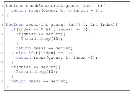
1) CheckSecret, a password-checker that compares a “guess” with an internally stored password, “secret” (see Figure 2), encoded as numbers. The program goes recursively over the elements of an arrayt of random boolean variables. The size refers to the length of array
t. Our techniques discovered a timing side-channel caused by the delays in the code.
1 boolean checkSecret(int guess, int[] t){ return recur(guess, t, t.length - 1);
3 }
5 boolean recur(int guess, int[] t, int index){ if(index == 0 && t[index] == 1){
7 if(guess <= secret){ Thread.sleep(10);
9 }
return guess == secret;
11 } else if(t[index] == 1){
return recur(guess, t, index -1);
13 }
if(guess <= secret){
15 Thread.sleep(10); }
17 return guess == secret; }
Figure 2: TheCheckSecretexample. One of the example programs that we investigate in Section 8.
which implements string compression using the Lempel-Ziv (LZ77) algorithm. We studied both a deterministic and a randomized version: with a probability p = 3/10, k = 1 bytes are appended to the compressed string before it is sent. The size here refers to the the number of characters of high and low strings (i.e., input lengths, which we kept equal for simplicity); our techniques discovered a space side channel, that reveals the secret through the size of the compressed input.
3) LawDB, a network service application that manages information about law enforcement personnel. Each employee’s data is referenced with a unique employee ID. Standard users are provided operations such as SEARCH and VIEW to manage information about employees except for the ones working on confidential activities. IDs of this particular group of employees are restricted. The requests handling non-confidential records are randomly delayed. In this case, “size” indi-cates the number of IDs in the database. Our techniques reported a timing channel in the process of handling a SEARCH request that is caused by additional com-putation, leading to slower response, when there are restricted IDs within the requested search range. 4) Collab, a complex application implementing a
net-work service that provides event scheduling. Users can insert events into theCollabcalendar. The events are organized by their ID in a re-balancing tree structure. In addition to regular users, Collab also has special auditorsthat can insert auditing events for other users. It is not possible for regular users to obtain auditing events directly. The application performs logging dur-ing the maintenance of the balanced tree. A random number determines how many lines are written to the log file. Our analysis identified both a timing and a space channel that reveals the IDs related to a user’s audits. This is due to the fact that when each node exceeds a certain number of IDs, the node is split into
two, which results in some extra logging, hence taking additional time.
8.1. Full Exploration of Symbolic Paths
We first evaluated our exact approach. The results are summarized in Table 1. For each example, we report the number of paths (#PC), the Shannon and the min-entropy leakages, along with the corresponding execution time. To illustrate the scaling behavior of our approach, we examined our examples for different size configurations.
For theCRIMEexample, we ran experiments on both the deterministic and the randomized versions (columns marked as CRIME and noisy CRIME): the results show that, as expected, the randomized version has smaller leakage for both Shannon and min-entropy measures.
8.2. Symbolic Path Sampling
We also experimented with our sampling approach on these examples. Figure 3 plots the lower and upper bounds of Shannon leakage for CRIME as more path samples (shown in percentage on x axis) are analysed. The plot shows how all the bounds converge to the exact leakage. Furthermore, if at any time the exploration is stopped, the real value of leakage is guaranteed to be between the lower and upper-bounds. A similar pattern was observed for all the other examples (see e.g. Figure 5 forCheckSecret). We observe that many samples are needed for the tight bound US tight* (given by Proposition 5) to get close to
the real value. If a bound on the number of observables is known, then a trivial upper-bound on the leakage is the “capacity” bound, i.e.,log2|O|. This can be improved
using Proposition 6 to an upper-bound that monotonically decreases to the exact leakage (marked asUSusing|O|). The LS tight is as provided by Proposition 7, whose tightness
comes from Proposition 8. Finally, “LS simple” is as per
(14), which is of course not as good as the “LS tight”.
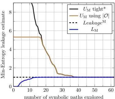
The plots for min-entropy are illustrated in e.g. Figures 6 (see also Fig. 4 forCheckSecret). The plots show how all the bounds converge to the exact leakage faster than the Shannon leakage case. Note also that our results can be used for side channeldetection. For example, if the lower bound for min-entropy leakage is greater than zero, then that means both min-entropy leakage and Shannon leakage are greater than zero, hence we can use the lower bound for min-entropy leakage todetect side channels. Thus, even if the bound is not tight, it can be very useful in practice.
8.3. Comparison with “Leakwatch”
CheckSecret CRIME noisyCRIME LawDB Collab
Size 100 150 200 3 4 3 4 200 300
#P C 202 302 402 77 799 154 1598 615 1030 2510
Shannon 0.46757 0.46757 0.46757 0.84290 0.92850 0.43598 0.49412 0.77320 1.14203 0.99712
Time 99 364 943 4 36 5 49 106 404 472
Min-Ent. 0.99930 0.99930 0.99930 0.92850 1.00000 0.76553 0.76553 3.32193 3.32193 1.0000
Time 107 412 920 4 37 5 49 158 388 515
TABLE 1: Computation of Shannon and min-entropy leakages using symbolic execution and model counting by Barvinok, for our four example case studies. Leakages are measured in bits, times in seconds.
0 20 40 60 80 100 0
2 4 6 8
% input space explored
Shannon
leak
age
estimate
UStight*
capacity USusing|O|
LeakageS
LStight
LSsimple
Figure 3: Shannon leakage estimates forCRIME(size 3).
0 20 40 60 80 100 120 140 0
2 4 6 8
number of symbolic paths explored
Min-En
trop
y
leak
age
es
ti
m
ate
UMtight*
UMusing|O|
LeakageM
LM
Figure 4: Min-entropy leakage estimates forCRIME(size3).
“Leakwatch” runs using its default settings. Notice first that, for this program, the leakage reported by the symbolic sampling is the real one (the approach coverges quickly); hence we observe that “Leakwatch” wrt symbolic sampling can be very imprecise. In particular in four out of thirteen cases “Leakwatch” wrongly report an absence of leakage: these false negatives can have serious security consequences, and could allow an attacker to go unnoticed and, with repeated runs, obtain the whole password. The second
obser-0 20 40 60 80 100 0
2 4 6 8
% input space explored
Shannon
leak
age
estimate
UStight*
capacity USusing|O|
LeakageS
LStight
LSsimple
Figure 5: CheckSecret’s Shannon leakage estimates (guess=1000,D={0, . . . ,10000}, size oft= 10).
0 10 20 30 40 50 60 0
2 4 6 8
number of symbolic paths explored
Min-En
trop
y
leak
age
es
ti
m
ate
UMtight*
UMusing|O|
LeakageM
LM
Figure 6: Estimates ofCheckSecret’s min-entropy leak-age (guess=1000,D={0, . . . ,10000}, size oft=30).
Guess Values
10 100 300 500 1000 3000 5000 8000 9000 9800 9900 9980 9990
LW Leak 0 0 0.1098 0.2008 0.3840 0.7954 0.9155 0.6410 0.3858 0.0633 0.0044 0 0 Time 16m29 21m9 21m22 22m1 11m22 11m8 11m54 15m1 11m35 13m27 14m46 20m23 13m16
SPF Leak 0.0114 0.0806 0.1939 0.2856 0.4676 0.8776 0.9944 0.7145 0.4617 0.1358 0.0761 0.0181 0.0094 Time 6.465 6.524 6.437 6.544 6.384 5.992 6.849 6.956 7.204 7.244 6.955 6.496 7.15
TABLE 2: Comparison of Shannon leakage evaluation for theCheckSecretexample (Figure 2) using “Leakwatch” (LW) and symbolic sampling in SPF. Notice time for Leakwatch is in minutes
.
9. Related Work
Symbolic analysis of side channels has been studied in [36], [37]. While these works share a similar symbolic execution platform with our approach, they do not address probabilistic programs or symbolic sampling.
Another related approach [23] uses symbolic analysis and Barvinok model counting to quantify information leak-age. That approach is based on a deductive verification system (KeY), and is not fully automated, as it requires user annotations for the KeY proofs. The work applies only to deterministic programs; it translates source code into a logical formula over which projection and model counting are applied; it is not clear how it could be applied to prob-abilistic programs. They also do not study any sampling.
There have been recent works quantifying leakage using Monte Carlo sampling, e.g. “Leakwatch” [9] and hybrid approaches where sampling is only performed under some conditions, e.g. [19]. However these approaches are based on standard sampling techniques, they are not symbolic and hence of a different nature to ours. Also our symbolic framework allows us to prove stronger theoretical guarantees compared to previous sampling techniques.
There is a significant literature on side-channel analysis, for example [3], [7], [8], [13], [24], [25], [31]. Recent works successfully use abstract interpretation for cache side-channels analysis [14], [26], [30]. Our approach differs from these works by using symbolic execution, symbolic sampling and considering probabilistic behavior.
Probabilistic programs are studied in [28], [32] in the context of enforcement [32] and synthesis [28] of privacy policies, where quantification of leakage becomes relevant. However compared to those works, our focus is on efficient quantification of leakage of side channels: it is not clear how those works advance on this problem. The case studies therein are quite small and even the greedy algorithm Syn-Grd in [28] relies on computing all observables, which can be prohibitively costly in practice.
Our lower bounds for min-entropy leakage are similar to the iterative approach in [4]. However that paper abstracts information systems into channel matrices whereas we de-velop a concrete program analysis. Moreover, we consider both min-entropy and Shannon leakages.
Symbolic execution and sampling are also used in [27] with proved bounds for Shannon and min-entropy leakages.
However that work considers standard sampling and applies only to deterministic systems; our bounds are for noisy systems and symbolic sampling. Noise introduces some significant technical challenges; also results on standard sampling do not hold for symbolic sampling, hence these works complement each other. Another work [33] provides bounds on information leakage from a sampling analysis, but it only applies to deterministic systems.
Our symbolic sampling is similar to previous work on probabilistic symbolic execution [17] which was done in the context of software safety and reliability. In this paper we provide novel results that allow us to use the information collected with symbolic sampling to compute theoretical lower- and upper- bounds on information leakage.
Conclusion
We presented a symbolic technique for computing leak-age in noisy side-channels. We also presented a sampling approach to scale up the technique, and provided upper and lower bounds to the leakage. Future work involves investigating model counting procedures for non-linear con-straints [5], [6] which will allow us to expand the appli-cability of the presented techniques to e.g. cryptographic protocols. We also plan to explore distributed versions of our techniques to further increase scalability.
Acknowledgment.We would like to thank the anonymous reviewers for their valuable comments. This material is based on research sponsored by DARPA under agreement number FA8750-15-2-0087. The U.S. Government is autho-rized to reproduce and distribute reprints for Governmental purposes notwithstanding any copyright notation thereon.
References
[1] Barvinok library. http://garage.kotnet.org/∼skimo/barvinok/.
[2] Giovanni Agosta, Luca Breveglieri, Gerardo Pelosi, and Israel Koren. Countermeasures against branch target buffer attacks, 2007.
[4] Miguel E Andr´es, Catuscia Palamidessi, Peter Van Rossum, and Ge-offrey Smith. Computing the leakage of information-hiding systems. InTACAS, pages 373–389. Springer, 2010.
[5] Mateus Borges, Antonio Filieri, Marcelo d’Amorim, Corina S. P˘as˘areanu, and Willem Visser. Compositional Solution Space Quan-tification for Probabilistic Software Analysis. InProc. of 35thACM SIGPLAN Conf. on Programming Language Design and Implemen-tation, PLDI ’14, pages 123–132, New York, NY, USA, 2014. ACM. [6] Mateus Borges, Quoc-Sang Phan, Antonio Filieri, and Corina S. P˘as˘areanu. Model-counting approaches for nonlinear numerical con-straints. In NASA Formal Methods: 9th International Symposium, NFM 2017, Moffett Field, CA, USA, May 16-18, 2017, Proceedings, pages 131–138. Springer International Publishing, 2017.
[7] David Brumley and Dan Boneh. Remote Timing Attacks Are Prac-tical. In Proc. of the 12th Conf. on USENIX Security Symposium -Volume 12, SSYM’03, Berkeley, CA, USA, 2003. USENIX Associ-ation.
[8] Shuo Chen, Rui Wang, XiaoFeng Wang, and Kehuan Zhang. Side-Channel Leaks in Web Applications: A Reality Today, a Challenge Tomorrow. In Proc. of the 2010 IEEE Symposium on Security and Privacy, SP ’10, pages 191–206, Washington, DC, USA, 2010. IEEE Computer Society.
[9] Tom Chothia, Yusuke Kawamoto, and Chris Novakovic. LeakWatch: Estimating Information Leakage from Java Programs. In 19th Eu-ropean Symposium on Research in Computer Security - Volume 8713, ESORICS 2014, pages 219–236, New York, NY, USA, 2014. Springer-Verlag New York, Inc.
[10] Thomas M. Cover and Joy A. Thomas. Elements of information theory. Wiley-Interscience, New York, NY, USA, 1991.
[11] Mark De Berg, Otfried Cheong, Marc Van Kreveld, and Mark Over-mars. Computational Geometry: Introduction. Springer, 2008.
[12] Leonardo De Moura and Nikolaj Bjørner. Z3: an efficient SMT solver. InProc. of the 14thinternational Conf. on Tools and algorithms for the construction and analysis of systems, TACAS’08, pages 337–340, Berlin, Heidelberg, 2008. Springer-Verlag.
[13] Quoc Huy Do, Richard Bubel, and Reiner H¨ahnle. Exploit Generation for Information Flow Leaks in Object-Oriented Programs. In ICT Systems Security and Privacy Protection: 30thIFIP TC 11 Intl. Conf., SEC 2015, Hamburg, Germany, pages 401–415. Springer, 2015. [14] Goran Doychev, Dominik Feld, Boris K¨opf, Laurent Mauborgne, and
Jan Reineke. CacheAudit: A Tool for the Static Analysis of Cache Side Channels. InProc. of 22ndUSENIX Conf. on Security, SEC’13,
pages 431–446, Berkeley, CA, USA, 2013. USENIX Association. [15] Thai Duong and Juliano Rizzo. The CRIME attack. InPresentation
at ekoparty Security Conf., 2012.
[16] Antonio Filieri, Corina S. P˘as˘areanu, and Willem Visser. Reliability analysis in symbolic pathfinder. InProc. of the 2013 International Conf. on Software Engineering, ICSE ’13, pages 622–631, Piscat-away, NJ, USA, 2013. IEEE Press.
[17] Antonio Filieri, Corina S. P˘as˘areanu, Willem Visser, and Jaco Gelden-huys. Statistical Symbolic Execution with Informed Sampling. In
Proc. of the 22Nd ACM SIGSOFT International Symposium on Foun-dations of Software Engineering, FSE 2014, pages 437–448, New York, NY, USA, 2014. ACM.
[18] Jaco Geldenhuys, Matthew B. Dwyer, and Willem Visser. Probabilis-tic Symbolic Execution. InProc. of the 2012 International Symposium on Software Testing and Analysis, ISSTA 2012, pages 166–176, New York, NY, USA, 2012. ACM.
[19] Yusuke Kawamoto, Fabrizio Biondi, and Axel Legay. Hybrid Statis-tical Estimation of Mutual Information for Quantifying Information Flow. In FM, volume 9995 ofLecture Notes in Computer Science, pages 406–425, 2016.
[20] John Kelsey. Compression and Information Leakage of Plaintext. In Revised Papers from the 9th International Workshop on Fast Software Encryption, FSE ’02, pages 263–276, London, UK, UK, 2002. Springer-Verlag.
[21] MHR Khouzani and Pasquale Malacaria. Leakage-Minimal Design: Universality, Limitations, and Applications. In30th IEEE Computer Security Foundations Symposium (CSF’17), 2017.
[22] James C. King. Symbolic execution and program testing. Commun. ACM, 19(7):385–394, July 1976.
[23] Vladimir Klebanov. Precise quantitative information flow analysis– a symbolic approach. Theoretical Computer Science, 538:124–139, 2014.
[24] Paul C. Kocher. Timing Attacks on Implementations of Diffie-Hellman, RSA, DSS, and Other Systems. InProc. of the 16thAnnual International Cryptology Conf. on Advances in Cryptology, CRYPTO ’96, pages 104–113, London, UK, UK, 1996. Springer-Verlag.
[25] Boris K¨opf and David Basin. An Information-theoretic Model for Adaptive Side-channel Attacks. InProc. of the 14thACM Conf. on Computer and Communications Security, CCS ’07, pages 286–296, New York, NY, USA, 2007. ACM.
[26] Boris K¨opf, Laurent Mauborgne, and Mart´ın Ochoa. Automatic quantification of cache side-channels. InProc. of the 24th interna-tional Conf. on Computer Aided Verification, CAV’12, pages 564– 580, Berlin, Heidelberg, 2012. Springer-Verlag.
[27] Boris K¨opf and Andrey Rybalchenko. Approximation and Ran-domization for Quantitative Information-Flow Analysis. InProc. of the 23rd IEEE Computer Security Foundations Symposium, CSF’10,
pages 3–14, Washington, DC, USA, 2010. IEEE Computer Society.
[28] Martin Kuˇcera, Petar Tsankov, Timon Gehr, Marco Guarnieri, and Martin Vechev. Synthesis of probabilistic privacy enforcement, 2017.
[29] Pasquale Malacaria. Algebraic foundations for quantitative informa-tion flow.Mathematical Structures in Computer Science, 25:404–428, February 2015.
[30] Heiko Mantel, Alexandra Weber, and Boris K¨opf. A Systematic Study of Cache Side Channels Across AES Implementations, 2017.
[31] Piotr Mardziel, M´ario S. Alvim, Michael W. Hicks, and Michael R. Clarkson. Quantifying Information Flow for Dynamic Secrets, 2014.
[32] Piotr Mardziel, Stephen Magill, Michael Hicks, and Mudhakar Sri-vatsa. Dynamic enforcement of knowledge-based security policies using probabilistic abstract interpretation. Journal of Computer Se-curity, 21(4):463–532, 2013.
[33] Stephen McCamant and Michael D. Ernst. Quantitative information flow as network flow capacity, 2008.
[34] David Molnar, Matt Piotrowski, David Schultz, and David Wagner. The program counter security model: Automatic detection and re-moval of control-flow side channel attacks, 2005.
[35] S Alvim M’rio, Kostas Chatzikokolakis, Catuscia Palamidessi, and Geoffrey Smith. Measuring information leakage using generalized gain functions, 2012.
[36] Quoc-Sang Phan, Lucas Bang, Corina S. P˘as˘areanu, Pasquale Malacaria, and Tevfik Bultan. Synthesis of Adaptive Side-Channel Attacks, August 2017.
[37] Corina S. P˘as˘areanu, Quoc-Sang Phan, and Pasquale Malacaria. Multi-run Side-Channel Analysis Using Symbolic Execution and Max-SMT, June 2016.
[38] Corina S. P˘as˘areanu, Willem Visser, David Bushnell, Jaco Gelden-huys, Peter Mehlitz, and Neha Rungta. Symbolic PathFinder: inte-grating symbolic execution with model checking for Java bytecode analysis.Automated Software Engineering, pages 1–35, 2013.
[39] Ashay Rane, Calvin Lin, and Mohit Tiwari. Raccoon: Closing Digital Side-channels Through Obfuscated Execution, 2015.