David Cash1, Feng-Hao Liu2, Adam O’Neill3, Mark Zhandry4, Cong Zhang5 1 Department of Computer Science, University of Chicago
2
Department of Computer and Electrical Engineering, Florida Atlantic University 3
Department of Computer Science, Georgetown University 4
Department of Computer Science, Princeton University 5
Department of Computer Science, Rutgers University
Abstract. Order-revealing encryption (ORE) is a popular primitive for outsourcing encrypted databases, as it allows for efficiently performing range queries over encrypted data. Unfortunately, a series of works, start-ing with Naveedet al.(CCS 2015), have shown that when the adversary has a good estimate of the distribution of the data, ORE provides little protection. In this work, we consider the case that the database entries are drawn identically and independently from a distribution of known shape, but for which the mean and variance are not (and thus the at-tacks of Naveedet al.do not apply). We define a new notion of security for ORE, calledparameter-hiding ORE, which maintains the secrecy of these parameters. We give a construction of ORE satisfying our new definition from bilinear maps.
Keywords.Encryption, Order-revealing encryption
1
Introduction
An emerging area of cryptography concerns the design and analysis of “leaky” protocols (see e.g. [33, 36, 12] and additional references below), which are pro-tocols that deliberately give up some level of security in order to achieve better efficiency. One important tool in this area is order-revealing encryption [8, 9].6. Order-revealing encryption (ORE) is a special type of symmetric encryption which leaks the order of the underlying plaintexts through a public procedure Comp. In practice, ORE allows for a client to store a database on an untrusted server in encrypted form, while still permitting the server to efficiently perform various operations such as range queries on the encrypted data without the secret decryption key. ORE has been implemented and used in real-world encrypted database systems, including CryptDB [36]
Various notions of ORE have been proposed. The strongest, called “ideal” ORE, insists that everything about the plaintexts is hidden, except for their order. For example, it should be impossible to distinguish between encryptions of 1,2,3 and 1,4,9. Such ideal ORE can be constructed from multilinear maps [9], showing that in principle ideal ORE is achievable. However, current multilinear
6
maps are quite inefficient, and moreover have been subject to numerous attacks (e.g. [16, 32, 17]).
In order to develop efficient schemes, the community often relaxes the security requirements, allowing for somewhat more leakage. Order-preserving encryption (OPE) [1, 7] — which actually predates ORE — is one example, whereCompis simply integer comparison. Very efficient constructions of OPE are known [7]. However, OPE necessarily leaks much more information about the plaintexts [7] than ideal ORE; intuitively, the difference between ciphertexts can be used to approximate the difference between the plaintexts. More recently, there have been efforts to achieve better security without sacrificing too much efficiency: Chenette, Lewi, Weis and Wu (CLWW) [15] recently gave an ORE construc-tion which leaks only the posiconstruc-tion of the most significant differing bits of the plaintexts.
Unfortunately, even hypothetical ideal ORE has recently been shown insecure for various use cases [24, 25, 3, 19, 30, 26, 11, 34, 20, 22]. This is even if the scheme itself reveals nothing but the order of the plaintexts. The problem is that just the order of plaintexts alone can already reveal a significant amount of information about the data. For example, if the data is chosen uniformly from the entire domain, then even ideal ORE will leak the most significant bits. As the most significant bits are often the most important ones, this is troubling.
The problem is that the definitions of ORE, while precise and provable, do not immediately provide any “semantically meaningful” guarantees for the privacy of the underlying data. Indeed, the above attacks show that when the adversary has a strong estimate of the prior distribution the data is drawn from, essentially no security is possible. However, we contend that there are scenarios (see below) where the adversary lacks this knowledge. A core problem in such scenarios is that the privacy of one message is inherently dependent on what other cipher-texts the adversary sees. Analyzing these correlations under arbitrary sources of data, even for ideal ORE, can be quite difficult. Only very mild results are known, for example the fact that either CLWW leakage or ideal leakage provably hides theleastsignificant bits of uniformly chosen data. Unfortunately, these bits are probably of less importance.
Therefore, a central goal of this paper is to devise a semantically meaningful notion of privacy for the underlying data in the case that the adversary does not have a strong estimate of the prior distribution, and develop a construction attaining this notion not based on multilinear maps.
We stress that we are not trying to devise a scheme that is secure in the use cases of the attacks above, as many of the attacks above would apply to any
ORE scheme; we are instead aiming to identify settings where the attacks do not apply, and then provide a scheme satisfying a given notion of security in this setting.
1.1 This Work: Parameter-Hiding ORE
distribution they came from. We show how to protect some information about the underlying data distribution.
Motivating Example. To motivate our notion, consider the following setting. A large university wants to outsource its database of student GPAs. For simplicity, we will assume each student’s academic ability is independent of other students, and that this is reflected in the GPA. Thus, we will assume that each GPA is sampled independently and identically according to some underlying distribu-tion. The university clearly wants to keep each individual’s GPA hidden. It also may want aggregate statistics such as mean and variance to be hidden, perhaps to avoid getting a reputation for handing out very high or very low grades.
Distribution-Hiding ORE. This example motivates a notion of distribution-hiding ORE, where all data is sampled independently and identically from some underlying distribution D, and we wish to hide as much as possible about D. We would ideally like to handle arbitrary distributions D, but in many cases will accept handling certain special classes of distributions. Notice that if the distribution itself is completely hidden, then so to is every individual record, since any information about a record is also information aboutD.
We begin with the following trivial observation: if D has high min-entropy (namely, super-logarithmic), then the ideal ORE leakage is just a random order-ing with no equalities, since there are no collisions with overwhelmorder-ing probability. In particular, this leakage is independent of the distribution D; as such, ideal ORE leakage hides everything about the underlying distribution, except for the super-logarithmic lower bound on min-entropy. Thus, we can use the multilinear map-based scheme of [9] to achieve distribution-hiding ORE for any distribution with high min-entropy.
We note the min-entropy requirement is critical, since for smaller min-entropies, the leakage allows for determining the frequency of the most common elements, hence learning non-trivial information aboutD.7
Unfortunately, the only way we know to build distribution-hiding ORE is using ideal leakage as above; as such, we do not know of a construction not based on multilinear maps. Instead, in hopes of building such a scheme, we will allow some information about the distribution to leak.
on an approximately normal distribution, so GPAs might reasonably be conjec-tured to be normal. For a different example, insurance claims are often modeled according to the Gamma distribution.
Therefore, since the general shape of the distribution is typically known, a reasonable relaxation of distribution-hiding ORE is what we will call parameter-hiding ORE. Here, we will assume the distribution has aknown, public “shape” (e.g. normal, uniform, Laplace etc.) but it may be shifted or scaled. We will allow the overall shape to be revealed; our goal instead is to completely hide the shifting and scaling information. More precisely, we consider a distribution D over [0,1] which will describe the general shape of the family of distributions in question. For example, if the shape in consideration is the set of uniform distributions over an interval, we may take D to be uniform distribution over [0,1]; if the shape is the normal distribution, we will take D be be the normal distribution with mean 1/2, and standard deviation small enough so that the vast majority of the mass is in [0,1]. LetDα,β be the distribution defined as: first samplex←D, and then outputbαx+βc. We will callαthe scaling term andβ the shift. The adversary receives a polynomial number of encryptions of plaintext sampled iid from Dα,β for someα, β. We will call a schemeparameter hiding if the scale and shift are hidden from any computationally bounded adversary. Our main theorem is that it is possible to construct such parameter-hiding ORE from bilinear maps:
Theorem 1 (Informal). Assuming bilinear maps, it is possible to construct parameter-hiding ORE for any “smooth” distribution D, provided the scaling term is “large enough.”
We note the restrictions to large scalings are inherent: any small scaling will lead to a distribution with low min-entropy. As discussed above, even with ideal ORE, it is possible to estimate the min-entropy of low min-entropy distributions, and hence it would be possible to recover the scaling term if the scaling term is small. Some restrictions on the shape ofD are also necessary, as certain shapes can yield low min-entropy even for large scalings. “Smoothness” (which we will define as having a bounded derivative) guarantees high min-entropy at large scales, and is also important technically for our analysis.
1.2 Technical Overview
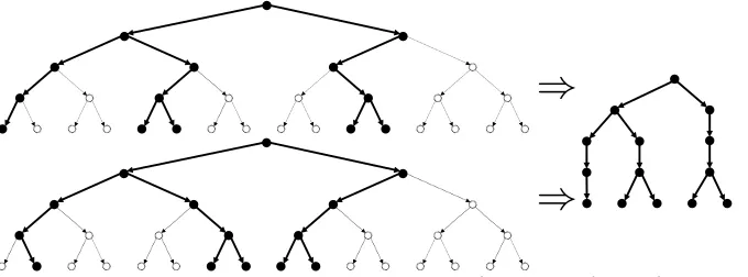
An alternative view of CLWW leakage Consider the plaintext space{0,1,2, . . . ,2`−1}. We will think of the plaintexts as leaves in a full binary tree of depth `. In this tree, the position of the most significant differing bit between two plain-texts corresponds to the depth of their nearest ancestor. The leakage of CLWW can therefore can be seen as revealing the tree consisting of all given plaintexts, their ancestors in the tree up to the lowest common ancestor, and the order of the leaves, with all other information removed. See Figure 1 for an illustration.
⇒
⇒
Fig. 1: CLWW Leakage. The two sets of plaintext {0,4,5,10,11} and {1,6,7,8,9}
correspond to equivalent subtrees. If the message space extends beyond 15, the CLWW leakage remains the same as depicted, since the leakage only reveals the tree up to the most recent ancestor.
Now, suppose all plaintext elements are in the range [0,2i) for somei. This means they all belong in the same subtree at heighti; in particular, the CLWW leakage will only have depth at mosti. Now, suppose we add a multiple of 2i to every plaintext. This will simply shift all the plaintexts to being in a different subtree, but otherwise keep the same structure. Therefore, the CLWW leakage will remain the same.
Therefore, while CLWW is not shift hiding, it isshift periodic. In particular, if imagine a distributionDwhose support is on [0,2i), and consider shiftingDby β. Consider an adversaryA, which is given the CLWW leakage fromqplaintexts sampled from the shifted D, and outputs a bit. If we plot the probability p(β) that A outputs 1 as a function of β, we will see that the function is periodic with period 2i.
Shift-Hiding ORE/OPE. With this periodicity, it is simple to construct a scheme that is shift hiding. To get a shift-hiding scheme for message space [0,2`), we instantiate CLWW with message space [0,2`+1). We also include as part of the secret key a random shift γ chosen uniformly in [0,2`). We then encrypt a messagemasEnc(m+γ). Adding a random shift can be seen as convolving the signal p(β) with the rectangular function
q(β) =
(
Since the rectangular function’s support matches the period ofp, the result is that the convolved signal ˆpisconstant. In other words, the adversary always has the same output distribution, regardless of the shift β. Thus, we achieve shift hiding.
When the comparison algorithm of an ORE scheme is simple integer compar-ison, we say the scheme is anorder-preserving encryption(OPE) scheme. OPE is preferable because it can be used without any modification to a database server. We recall that CLWW can be made into an OPE scheme — where ciphertexts are integers and comparision is integer comparison — while maintaining the CLWW leakage profile. Our conversion to shift-hiding preserves the OPE property, so we similarly achieve a shift-hiding OPE scheme.
Scale-Hiding ORE/OPE. We note that we can also turn any shift-hiding ORE into a scale-hiding ORE. Simply take the logarithm of the input before encrypt-ing; now multiplying by a constant corresponds to shifting by a constant. Of course, taking the logarithm will result in non-integers; this can easily be fixed by rounding to the appropriate level of precision (enough precision to guarantee no collisions over the domain) and scaling up to make the plaintexts integral. Similarly, we can also obtain scale-hiding OPE if we start with an OPE scheme.
Impossibility of parameter-hiding OPE. One may hope to achieve both shift-hiding and scale-shift-hiding by some combination of the two above schemes. For example, since orderpreserving encryption schemes can be composed, one can imagine composing a shift-hiding scheme with a scale-hiding scheme. Interest-ingly, this does not give a parameter-hiding scheme. The reason is that shifts/scalings of the plaintext do not correspond to shifts/scalings of the ciphertexts. There-fore, while the outer OPE may provide, say, shift-hiding for its inputs, this will not translate to shift-hiding of the inner OPE’s inputs.
Nonetheless, one may hope that tweaks to the above may give a scheme that is simultaneously scale and shift hiding. Perhaps surprisingly, we show that this is actually impossible. Namely, we show thatOPE cannot possibly be parameter-hiding. We prove this in appendix B. We first provide a simple proof of the impossibility of ideal security for OPE, re-proving [7, 15] but in a much simpler way. Our proof is flexible to the exact choice of plaintexts, and we then show how to extend it to parameter-hiding OPE, even when the adversary sees just two ciphertexts.
This impossibility shows that strategies leveraging CLWW leakage are un-likely to yield parameter-hiding ORE schemes. Interestingly, all ORE schemes we are aware of that can be constructed from symmetric crypto can also be made into OPE schemes. Thus, this suggests we need stronger tools than those used by previous efficient schemes.
Parameter Hiding via Smoothed CLWW Leakage Motivated by the
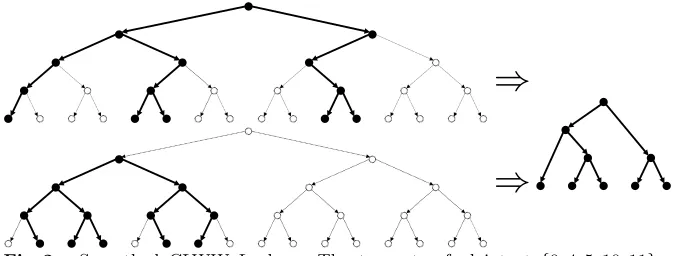
that will allow us to perform similar tricks as in the shift hiding case in order to achieve both scale and shift hiding simultaneously. Our dream leakage will be a “smoothed” CLWW leakage, where all nodes of degree exactly 2 are replaced with an edge between the two neighbors. In other words, the dream leakage is the smallest graph that is “homeomorphic” to the CLWW leakage. See Figure 2 for an illustration.
⇒
⇒
Fig. 2: Smoothed CLWW Leakage. The two sets of plaintext {0,4,5,10,11} and
{1,2,3,5,6}correspond to equivalent smoothed subtrees. Notice that the CLWW leak-age for these two trees is different.
Our key observation is that this smoothed CLWW leakage now exhibits ad-ditional periodicity. Namely, if we multiply every plaintext by 2, every edge in the bottom layer of the CLWW leakage will get subdivided into a path of length 2, but smoothing out the leakage will result in the same exact graph. This means that smoothed CLWW leakage is periodic in thelog domain.
In particular, if imagine a distribution D whose support is on [0,2i), and consider multiplying byα. Consider an adversaryA, which is given the smoothed CLWW leakage from qplaintexts sampled from a scaled D, and outputs a bit. If we plot the probabilityp(log2α) thatAoutputs 1 as a function ofα, we will see that the function is periodic with period 1.
Therefore, we can perform a similar trick as above. Namely, we convolvep with the uniform distribution over the period of p in the log domain. We ac-complish this by including a random scalar α as part of the secret key, and multiplying byαbefore encrypting. However, this time several things are differ-ent:
– Since we are working in the log domain, the logarithm of the random scalar αhas to be uniform. In other words,αis log-uniform
the period thatαapproximates the continuous log-uniform distribution sufficiently well.
• Second, unlike the shift case, sampling at random fromDand then scal-ing is not the same as samplscal-ing from a scaled version of D, since the rounding step does not commute with scaling. For example, for con-creteness consider the normal distribution. If we sample from a normal distribution (and round) and then scale, the resulting plaintexts will all be multiples of α. However, if we sample directly from a scaled nor-mal distribution (and then round), the support of the distribution will include integers which are not multiples ofα.
To remedy this issue, we observe that if the plaintexts are sampled from a wide enough distribution, their differing bits will not be amongst the lowest significant bits. Hence, the leakage will actually be independent of the lower order bits. For example, this means that while the rounding does not commute with the scaling, the leakage actually does not depend on the order in which the two operations are carried out.
• The above arguments can be made to work for, say, the normal dis-tribution. However, we would like to have a proof that works for any distribution. Unfortunately, for distributions that oscillate rapidly, we may run into trouble with the above arguments, since rounding such distributions can cause odd behaviors at all scales. This problem is actu-ally unavoidable, as quickly oscillating distributions may have actuactu-ally have low min-entropy even at large scales. Therefore, we must restrict to “smooth” functions that have a bounded derivative.
Using a careful analysis, we are able to show for smooth distributions that we achieve the desired scale hiding.
– Finally, we want to have a scheme that is both scale and shift hiding. This is slightly non-trivial, since once we introduce, say, a random shift, we have modified the leakage of the scheme, and cannot directly appeal to the argu-ments above to obtain scale hiding as well. Instead, we distill a set of specific requirements on the leakage that will work for both shift hiding and scale hiding. We show that our shift hiding scheme above satisfies the require-ments needed in order for us to introduce a random scale and additionally prove scale hiding.
Achieving Smoothed CLWW Leakage. Next we turn to actually construct-ing ORE with smoothed CLWW leakage. Of course, ideal ORE has better than (smoothed) CLWW leakage, so we can construct such ORE based on multilinear maps. However, we want a construction that uses standard tools.
We therefore provide a new construction of ORE using pairings that achieves smoothed CLWW leakage. We believe this construction is of interest on its own, as it is achieves the to-date smallest leakage of any non-multilinear map based scheme.
(basic) scheme, the encryption key is just a PRF keyK. To encrypt a plaintext x∈ {0,1}n, for each prefixp
i=x[1, . . . , i], the scheme computes yi=PRFK(pi) +xi+1
wherexi+1 is the (i+ 1)-st bit of x, and the output of PRF∈ {0,1}λ is treated as an integer (we will takeλto be the security parameter). The ORE ciphertext is then (y1. . . , yn). To compare two ciphertexts (y1. . . , yn) and (y01. . . , y0n), one finds the smallest indexi such thatyi 6=y0i, and outputs 1 ify0i−yi = 1. This naturally reveals the index of the bit where the plaintexts differ.
Our approach to reducing the leakage is to attempt to hide the indexiwhere the plaintexts differ. As a naive attempt at this, first consider what happens if we modify the scheme to simply randomly permute the outputs (y1. . . , yn) (with a fresh permutation chosen for each encryption). We can still compare ciphertexts by appropriately modifying the comparison algorithm: now givenc= (y1. . . , yn) and c0 = (y10. . . , yn0) (permuted as above), it will look for indices i, j such that either y0i−yj = 1, in which case it outputs 1, or yj−yi0 = 1, in which case it outputs 0. (If we choose the output length of the PRF to be long enough then this check will be correct with overwhelming probability.)
This modification, however, does not actually reduce leakage: an adversary can still determine the most significant differing bit by counting how many ele-mentscandc0 have in common.
We can however recover this approach by preventing an adversary from de-tecting how many elementscandc0have in common. To do so, we employ a new notion of property-preserving hashing (PPH) we introduce. Intuitively, a PPH is a randomized hashing scheme that is designed to publicly reveal a particular predicateP on pairs of inputs.
PPH can be seen as the hashing (meaning, no decryption) analogue of the notion of property-preserving encryption, a generalization of order-revealing en-cryption to arbitrary properties due to Pandey and Rouselakis [35]. (This can also be seen as a symmetric-key version of the notion of “relational hash” due to Mandal and Roy [31].)
Specifically, we construct and employ a PPH for the property
P1(x, x0) =
(
1 ifx=x0+ 1 0 otherwise
(Herex, x0 are not plaintexts of the ORE scheme, think of them as other inputs determined below.) Security requires that this isall that is leaked; in particular, input equality is not leaked by the hash values (which requires a randomized hashing algorithm).
yi’s.8The comparison algorithm can again be modified appropriately, namely to not to check ify0i−yj = 1 but rather if their h0i andh0j hash values satisfy P1 via the PPH (and similarly for the checkyj−yi0= 1).
For any two messages, the resulting ORE scheme is actually ideal: it only reveals the order of the underlying plaintexts, but nothing else. However, for three messages m, m0, m00 we see that some additional information is leaked. Namely, if we find thatyi0−yj= 1y00k−yj= 1, then we know thatyj0 =yk00. We choose the range of the PRF large enough so that this can only happen ifyj0 and yk0 are bothPRFK(p`) +x`+1 for the same prefixp` and same bit x`+1, andy0j corresponds to the most significant bit wherem0 differs fromm,yk00corresponds to the most significant bit wherem00differs fromm, and moreover these positions are the same. Therefore, the adversary learns whether these most-significant differing bits are the same. It is straightforward to show that this leakage is exactly equivalent to the smoothed CLWW leakage we need. Proving this ORE scheme secure wrt. this leakage based on an achievable notion of security for the PPH turns out to be technically challenging. Nevertheless, we manage to prove it “non-adaptively secure,” meaning the adversary is required to non-adaptively choose the dataset, which is realistic for a passive adversary in the outsourced database setting.
Property-preserving hash from bilinear maps. Next we turn to constructing a property-preserving hash (PPH) for the property P1(x, x0) = x =x0+ 1. For this, we adapt techniques from perfectly one-way hash functions [10, 31] to the symmetric-key setting and use asymmetric bilinear groups. Roughly, in our con-struction the key for the hash function is a keyK for a pseudorandom function PRF and, letting e: G1×G2 → GT be an asymmetric bilinear map on prime order cyclic groupsG1, G2 with generators g1, g2, the hash ofxis
HK(x) = (g1r1, g
r1PRFK(x)
1 , g
r2 2 , g
r2PRFK(x+1)
2 )
for fresh randomr1, r2∈Zp. (Thus, the PRF is also pushed to our PPH construc-tion and can be dropped from from the higher-level ORE scheme when our hash function is plugged-in.) The bilinear map allows testing whether P1(x, x0) from HK(x),HK(x0), and intuitively our use of asymmetric bilinear groups prevents testing other relations such as equality (formally we use the XSDH assumption). We prove the construction secure under an indistinguishability-based notion in which the adversary has to distinguish between the hash of a random challenge x∗ and a random hash value, and can query for hash values of inputs xof its choice as long asP1(x, x∗) andP1(x∗, x) are both 0. Despite being restricted,9, this notion suffices in our ORE scheme above.
8
A minor issue here is that we now lose decryptability for the resulting ORE scheme; however, this can easily be added back in a generic way by also encrypting the plaintext separately under a semantically secure scheme.
When our PPH is plugged-in to our ORE scheme, ciphertexts consist of 4n group elements, and order comparison requires n(n−1) pairing computations on average. We also note that CLWW gave an improved version of their scheme where ciphertexts are size O(n) rather than O(nλ) for security parameter λ, however, we have reason to believe this may be difficult for schemes with our improved leakage profile, see below.
Piecing everything together, we obtain a parameter-hiding ORE from bilinear maps. We note that, as parameter-hiding OPE is impossible, we achieve the first construction of ORE without multilinear maps secure with a security notion that is impossible for OPE.
Compare to concurrent work. In [29], the authors give an efficient ORE construction based on PRFs, while their leakage profile cannot achieve shift hid-ing and scale hidhid-ing simultaneously, which means their scheme cannot meet our privacy notion. Moreover, in [27], the authors give an alternative ORE construc-tion, based on pairings, while their leakage needs further analysis.
Generalizing our ORE scheme. In our work, we also show several extensions to our smoothed CLWW ORE scheme. In one direction, we show an improved leakage by considering blocks of bits at a time(encrypting message block by block, rather than bit by bit). And interestingly, we show that if the block size is only 2, then we improve security and efficiency simultaneously, while for larger block, the leakage continues to reduce but efficiency compared to the basic scheme (in terms of both ciphertext size and pairings required for comparison) decreases.
On the other hand, we also show how to improve efficiency while sacrificing some security. Interestingly, we are able to show a more efficient version of the scheme than above(only need O(n) pairings for each comparison), that is still sufficient for achieving parameter-hiding ORE using our conversion.
In addition, we also show how our ORE scheme easily gives aleft/right ORE
as defined by [29] that also improves on their leakage. In left/right ORE, cipher-texts can be generated in either the left mode or right mode, and the comparison algorithm only compares a left and a right ciphertext. Security requires that no information is leaked amongst left and right ciphertexts in isolation.
1.3 Discussion and Perspective
The original OPE scheme of [7] leaks “whatever a random order-preserving func-tion leaks.” Unfortunately, this nofunc-tion does not say anything about what such leakage actually looks like. The situation has been improved in recent works on OPE such as CLWW which define a precise “leakage profile” for their scheme. However, such leakage profiles are still of limited use, since they do not obviously say anything about the actual privacy of the underlying data.
claim security as long all that is sensitive is the scale and shift of the underlying plaintext distributions. If, for example, if the shape of the distribution is highly sensitive, or if there are correlations to other data available to the attacker, our notion is insufficient.
However, our construction provably has better leakage than existing efficient schemes, and it at least shows some meaningful security for specific situations. Moreover we suspect that the scheme can be shown to be useful in many other settings by extending our techniques.
1.4 Related Work
Work done on “leaky cryptography” includes work on multiparty computa-tion [33], searchable symmetric and structured encrypcomputa-tion [37, 21, 13, 18, 14, 12, 28], and property-preserving encryption [5, 7, 35]. In the database community, the problem of querying an encrypted database was introduced by Hacig¨um¨u¸s, Iyer, Li and Mehrotra [23], leading to a variety of proposals there but mostly lacking formal security analysis. Proposals of specific outsourced database sys-tems based on property-preserving encryption like ORE include CryptDB [36], Cipherbase [2], and TrustedDB [4].
2
Background
Notation. All algorithms are assumed to be polynomial-time in the security
parameter (though we will sometimes refer to efficient algorithms explicitly). We will denote the security parameter byλ. For a random variableY, we write y←$ Y to denote thaty is sampled according to Y’s distribution, moreover, let D be Y’s distribution, we abuse notation y ←$ D to mean that y is sampled according toD. For an algorithmA, by y←$ A(x) we mean thatA is executed on input x and the output is assigned to y, furthermore, if A is randomized, then we writey ← A($ x) to denote runningA on inputxwith a fresh random tape and letting y be the random variable induced by its output. We denote by Pr[A(x) = y : x ←$ X] the probability that A outputs y on input x when x is sampled according toX. We say that an adversary Ahas advantage in distinguishing X from Y if Pr[A(x) = 1 : x←$ X] and Pr[A(y) = 1 : y ←$ Y] differ by at most.
When more convenient, we use the following probability-theoretic notation instead. We write PX(x) to denote the probability that X places on x, i.e. PX(x) = Pr[X = x], and we say PX(x) is the probability density function (PDF) of X’s distribution. The statistical distance between X and Y is given by ∆ = 1
2
P
x|PX(x)−PY(x)|. If ∆(X, Y) is at most then we say X, Y are -close. It is well-known that ifX, Y are-close then any (even computationally unbounded) adversaryAhas advantage at mostin distinguishingX fromY.
0 faster than any polynomial in λ, i.e. ∀c > 0 ∃λ∗ ∈ N ∀λ ≥ λ∗ : |ν| ≤ 1 λc. We let [M] = {1, . . . , M}, [M]0 = {0, . . . , M−1} and [M, N] = {M, . . . , N}. We write m as a vector of plaintexts and |m| as the vector’s length, namely m= (m1, . . . , ms) and|m|=s. For a vectorm, byamwe mean (am1, . . . , ams) and we writem+bto denote (m1+b, . . . , ms+b). Letxbe a real number, we write bxcas the largest integer s.t.bxc ≤x, anddxeas the smallest integer s.t.dxe ≥x. Bybxe, we mean roundingxto the nearest integer, namely−1/2≤ bxe−x <1/2. If P is a predicate, we write 1(P) for the function that takes the inputs toP and returns 1 ifP holds and 0 otherwise.
PRFs. We use the standard notion of a PRF. A functionF : {0,1}λ×D →
{0,1}λis said to be aPRF with domainD if for all efficientAwe have that |Pr[AF(K,·)(1λ) = 1]−Pr[Ag(·)(1λ) = 1]|
is a negligible function of λ, where K is uniform over {0,1}λ and g is uniform over all functions fromDto {0,1}λ.
ORE. The following definition of syntax for order-revealing encryption makes
explicit that comparison may use helper information (e.g. a description of a particular group) by incorporating acomparison key, denoteck.
Definition 2 (ORE). A ORE scheme is a tuple of algorithms Π = (K,E,C)
with the following syntax.
– The key generation algorithm K is randomized, takes inputs (1λ, M), and always emits two outputs(sk,ck). We refer to the first outputskas thesecret keyand the second output ckas the comparison key.
– The encryption algorithm E is randomized, takes inputs (sk, m)where m∈ [M], and always emits a single outputc, that we refer to as a ciphertext. – The comparison algorithm C is deterministic, takes inputs (ck, c1, c2), and
always emits a bit.
If the comparison algorithmCis simple integer comparison (i.e., ifC(ck, c1, c2)
is a canonical algorithm that treats its the ciphertexts and binary representations of integers and tests which is greater) then the scheme is said to be an order-preserving encryption (OPE)scheme.
Correctness of ORE schemes.Intuitively, an ORE scheme is correct if the
comparison algorithm can output the order of the underlying plaintext, by taking ckand two ciphertexts as inputs.
We say that an ORE schemeΠ is computationally correct if for all efficient adversariesA, allM = poly(λ), we have that Pr[CORoreP i(A) = 1] is a negligible function in the security parameter.
Security of ORE schemes.The following simulation-based security definition is due to Chenette et al. [15]. Here aleakage profile is any randomized algorithm. The definition refers to games given in Figure 3, which we review now. In the real game, key generation is run and the adversary is given the comparison key and oracle access to the encryption algorithm with the corresponding secret key. The adversary eventually outputs a bit that the game uses as its own output. In the ideal simulation game, the adversary is interacting with the same oracle, but the comparison key is generated by a stateful simulator, and the oracle responses are generated by the simulator which receives leakage from the stateful leakage algorithmL.
Game REALoreΠ(A): (sk,ck)← K$ (1λ, M);b $
← AEnc(ck)
Returnb
Enc(m):
ReturnE(sk, m)
Game SIMoreΠ,L(A,S):
st`← ⊥; (ck,sts) $
←S(1λ);b $
← AEnc(ck)
Returnb
Enc(m):
(L,st`) $
← L(st`, m); (c,sts) $
← S(L,sts) Returnc
Fig. 3:Games REALoreΠ(A) (left) and SIMore
Π,L(A,S) (right), whereΠ = (E,C) is an
ORE scheme,Lis a leakage profile,Ais an adversary, andS is a simulator.
Definition 3 (L-simulation-security for ORE). For an ORE scheme Π, an adversary A, a simulator S, and leakage profile L, we define the games
REALoreΠ(A)andSIMoreΠ,L(A)in Figure 3. The advantage ofAwith respect to S
is defined as
AdvoreΠ,L,A,S(λ) =
Pr[REAL
ore
Π(A) = 1]−Pr[SIM ore
Π,L(A,S) = 1]
.
We say that Π is L-simulation-secure if for every efficient adversary A there exists an efficient simulatorS such thatAdvoreΠ,L,A,S(λ)is a negligible function.
We also define non-adaptive variants of the games where A gets a single query to an oracle that accepts a vector of messages of unbounded size. In the real game REALoreΠ-na(A), the oracle returns the encryptions applied independently to each message. In the ideal game SIMoreΠ-na(A), the leakage function gets the entire vector of messages as input and produces an output L that is then given toS which produces a vector of ciphertexts, which are returned by the oracle.
Ideal ORE. Ideal ORE is the case where the leakage profileLis simply the list of results of comparisons between the plaintexts. We note that such aLisalways
revealed by the comparison algorithm, so ideal ORE is the best one can hope for. Ideal ORE can be constructed from multilinear maps [9].
CLWW Leakage. As an example of a non-ideal leakage profile, consider the leakage Lclww of Chenette, Lewi, Weis and Wu [15]. For m0, m1 ∈ {0,1}n, we define the most significant differing bit of m1 and m2, denoted msdb(m0, m1), as the index of first bit wherem0, m1 differ, orn+ 1 if m1=m2.
The CLWW leakage profileLclww takes in input a vector of plaintextm = (m1, . . . , mq) and produce the following:
Lclww(m1, . . . , mq) := (∀1≤i, j≤n,1(mi< mj),msdb(mi, mj))
3
New Security Notions for ORE
In this section, we propose four meaningful notions of privacy: distribution-hiding,parameter-hiding,scale-hiding and shift-hiding; in those notions, we are considering the privacy of the underlying distribution of data records, rather than the individual data records, and show how to protect information about the underlying data distribution.
Distribution-Hiding for ORE.We assume that all database entries are
in-dependently and identically distributed according to some distribution D10, and the notion of distribution-hiding refers to game defined in Figure 4. In the inter-active game, after receiving the public parameter and comparison key, adversary Apicks two distributions D0, D1 and sends to challengerC, C then flips a coin b, samples a sequence of entries fromDb, and sends back the encrypted entries. EventuallyAoutputs a bit, and we say adversary wins if it guesses bcorrectly. We note that if either ofDbhas low min-entropy, it is possible for an adversary to estimate the min-entropy by looking for collisions in its ciphertexts. Therefore, we must restrictDb to have high min-entropy.
GameDHΠ,q(A, λ):
(sk,ck)← K$ (1λ, M);D0, D1← A(1λ,ck) s.t.H∞(Db)≥ω(logλ)
b← {$ 0,1},m←$ Dbs.t.|m|=q; maxDb≤M;c=E(sk,m)
b0=A(ck,c); Return (b=? b0)
Fig. 4:GamesDHΠ,q(A, λ) , whereΠ= (K,E,C) is an ORE scheme,q=poly(λ), and
Ais an adversary.
Definition 4 (Distribution-Hiding for ORE). For an ORE scheme Π, an adversary A, function q =q(λ) we define the gamesDHΠ,q(A, λ) in Figure 4.
The advantage of A is defined as AdvDHΠ,q(A, λ) = |Pr[DHΠ,q(A, λ)− 1 2]|. We
say that Π is distribution-hiding if for every efficient adversary A, and any polynomialq=poly(λ),AdvDHΠ,q(A, λ)is a negligible function.
We immediately observe that ideal ORE achieves distribution hiding, while for other known leakier ORE schemes, it’s seems unfeasible to achieve this privacy guarantee. However, in many settings, the general shape of the distribution is often known (that is, if the distribution is normal, uniform, Laplace, etc), and it is reasonable to allow the overall shape to be reveal but hide its mean and/or variance completely, subject to certain restrictions. Before formalize these notion, we firstly introduce some notations.
For a continuous random variableX, whereD isX’s distribution, we abuse notation pD(x) = pX(x). Now we introduce three alternative distributions: Dδscale, Dshift` , Daffδ,`with parameterδ, `, where the corresponding probability den-sity function is defined as:
pDscale= pD( x δ)
δ ; pDshift(x) =pD(x−`); pDaff =
pD(x−δ`) δ
In other words,Dδ
scale scales the shape ofDby a factor ofδ;Dshift shiftsD by` andDaff does both.
Rounded distribution.As our plaintexts are integers, we need map real num-ber to its rounded integer, namely x→ bxe. More precisely, let D be a distri-bution over real numbers between α and β; we induce a rounded distribution RDα,βon [dαe,bβc]which samples fromDand then rounds. Its probability density function is:
pRα,β D
(k) =
Rdαe+1/2 α pD(x)dx
Rβ αpD(x)dx
k=α Rk+1/2
k−1/2pD(x)dx Rβ
αpD(x)dx
k∈[dα+ 1e,bβ−1c] Rβ
bβc−1/2pD(x)dx Rβ
αpD(x)dx
k=β
0 Otherwise
In the case ofDδ scale,D
`
shift, orD δ,`
aff, we will use the notationbD δ
scalee,bD ` shifte, andbDaffδ,`eto denote the respective rounded distributions.
Now, we present the notion “(γ, D)-parameter-hiding” ORE, referring to the game defined in Figure 5. Here,D is a distribution over [0,1], which represents the description of the known shape of the distribution of plaintexts.γis a lower-bound on the scaling that is allowed. Then key generation is run and adversary is given the public parameter, (γ, D), and the comparison key. Then, the adversary A sends two pairs of parameters (δ0, `0),(δ1, `1) to challenger C. Next, C flips a coin b, checks whether the parameter is proper(1(δ0 ≥ γ∩δ1 ≥ γ) ), then samples a sequence of data entries from the rounded distribution bDδb,`b
sends back encrypted data. Eventually Aoutputs a bit, and we say adversary wins if it guessesbcorrectly.
Game (γ, D)-para-hidΠ,q(A, λ): (sk,ck)← K$ (1λ, M);δ
0, `0, δ1, `1← A(ck, D) Ifδ0< γ orδ1< γ, output a random bit and abort, else,b← {$ 0,1},m← b$ Dδb,`b
aff e, s.t.|m|=q; maxbD δb,`b
aff e ≤M;c=E(sk,m)
b0=A(ck,c) Return (b=? b0)
Fig. 5: Gamespara-hidΠ,q(A, λ) , whereΠ = (E,C) is an ORE scheme,D is a distri-bution on [0,1],Ais an adversary
Definition 5 ((γ, D)-parameter hiding for ORE).For an ORE schemeΠ, an adversary A, a distributionD, and function q=q(λ), we define the games
(γ, D)-para-hidΠ,q(A, λ) in Figure 5. The advantage ofA is defined as
AdvparaΠ,q,γ,D-hid(A, λ) =|Pr[(γ, D)-para-hidΠ,q(A, λ)− 1 2]|
We say thatΠ is(γ, D)-parameter hiding if for every efficient adversaryAand polynomialq AdvparaΠ,q,γ,D-hid(A, λ)is a negligible function.
Similarly, we define (γ, D)-scale hiding and (γ, D)-shift hiding with little change as above. More precisely, in the game of (γ, D)-scale hiding, we add the restric-tion`0=`1 = 0 and in the game of (γ, D)-shift hiding, we add the restriction δ0=δ1. Due to the space limit, we skip the formal definitions here.
We note that these three notions are distribution dependent, and we would like they work for any distribution. Unfortunately, quickly oscillating distribu-tions do not fit into our case, as they may have actually low min-entropy for their discretized distributions on integers, even at large scales. Hence, we place additional restrictions. We place the following restriction, which is sufficient, but potentially stronger than necessary:
(η, µ)-smooth distribution. We let D be a distribution where its support mainly on [0,1] (Pr[x /∈ [0,1] : x ← D] ≤ negl(λ)), we denote p0D(x) as its derivative, and we say that D is (η, µ)-smooth if 1)∀x∈ [0,1], pD(x) ≤η; 2) |p0D(x)| ≤η for allx∈[0,1] except forµpoints.
Definition 6 ((γ, η, µ)-parameter hiding for ORE). For an ORE scheme
4
Parameter Hiding ORE
In this section, we will assume we are given an ORE Π = (K,E,C) with a “smoothed” version of CLWW leakage, defined below. Later, in Section 5, we will show how to instantiate such a scheme from bilinear maps.
We show how to convert a scheme with smoothed CLWW leakage into a parameter-hiding ORE scheme by simply composing with a linear function: namely, for any plaintext m, the ciphertext has form E(αm+β), where α, β are the same across all messages and are sampled as part of the secret key. Intu-itively,αhelps to hide the scale parameter andβ hides the shift. We need to be careful about the distributions ofαandβ;αneeds to be drawn from a “discrete log uniform” distribution of appropriate domain, andβneeds to be chosen from a uniform distribution of appropriate domain.
The discrete log uniform distributionDon [A, B] (logU(A, B)) has probabil-ity densprobabil-ity function:
pD(k) =
( 1/k
PB i=A1/i
i∈[A, B]
0 Otherwise
We say a leakage functionLis smoothed CLWW if:
1. For any two plaintext sequences m0,m1, if Lclww(m0) = Lclww(m1), then L(m0) =L(m1) (in other words, it leaks no more information that CLWW); 2. For any plaintext sequence m,L(m) =L(2m)
4.1 Parameter-Hiding ORE
In this part, we give the formal description of parameter-hiding ORE. To simplify our exposition, we first specify some parameters. We will assume we are given:
q=poly(λ), M = 2poly(λ), γ= 2ω(logλ), η, µ≤O(1)
We will assumeγ andM are exactly powers of 2 without loss of generality by rounding up. We define:
τ =γ, ξ=γ2, U = 4ξM, T =γ2×U, K= 2×T
LetΠ = (K,E,C) be an ORE scheme on message space [K] with smoothed CLWW leakage L. We define our new ORE Πaff = (Kaff,Eaff,Caff) on message space [M] as follows:
– Eaff(skaff, m). On input the secret keyskaffand a messagem∈[M], it outputs CTaff=E(αm+β)
By our choice of message space [K] forΠ, the input toE is guaranteed to be in the message space.
– Caff(ckaff,CT0aff,CT 1
aff): On inputs the comparison key ckaff, two ciphertexts CT0aff,CT1aff, it outputsC(ckaff,CT0aff,CT1aff)
Here we also give the description of composted schemes that only achieve “scale-hiding” or “shift-hiding”. Formally, we defineΠscale= (Kscale,Escale,Cscale) andΠshift= (Kshift,Eshift,Cshift), respectively:
– Kscale(1λ, M, Π): On input the security parameterλ, the message space [M] andΠ, the algorithm picks a super-polynomialγ= 2ω(logλ)as a global pa-rameter, and computes parameters above. Then it runs (ck,sk)← K(1λ, K), drawsα←$ logU(ξ,2ξ−1) and outputsskscale= (sk, α),ckscale=ck;
– Escale(skscale, m). On input the secret keyskscale and a message m∈ [M], it outputs
CTscale=E(αm)
– Cscale(ckscale,CT0scale,CT 1
scale): On inputs the comparison key ckscale, two ci-phertextsCT0scale,CT1scale, it outputsC(ckscale,CT0scale,CT1scale).
– Kshift(1λ, M, Π): On input the security parameterλ, the message space [M] and Π, the algorithm picks a super-polynomial γ = 2ω(logλ) as a global parameter, and computes parameters above. Then it runs (ck,sk)← K(1λ), drawsβ from discrete uniform on [T]0 and outputsskshift = (sk, α),ckshift= ck;
– Eshift(skshift, m). On input the secret key skshift and a message m ∈ [M], it outputs
CTshift=E(m+b)
– Cshift(ckshift,CT0shift,CT 1
shift): On inputs the comparison keyckshift, two cipher-textsCT0shift,CT1shift, it outputsC(ckshift,CT0shift,CT1shift).
The correctness ofΠaff, Πscale andΠshift is directly held by correctness ofΠ, and what is more interesting is the privacy that those scheme can guarantee.
4.2 Main Theorem
In the part, we proveΠaff is parameter hiding, formally:
Theorem 7 (Main Theorem).Assuming Π has L-simulation-security where
L is smoothed CLWW, then for any γ = 2ω(logλ), Πaff is (γ, η, µ)-parameter
Proof. According to the security notions, it is straightforward that if an ORE scheme is (γ, η, µ)-parameter hiding, then it is also (γ, η, µ)-scale hiding and (γ, η, µ)-shift hiding. Next we claim the converse proposition holds.
Claim. If an ORE scheme Π achieves (γ, η, µ)-scale hiding and (γ, η, µ)-shift hiding simultaneously, thenΠ is (γ, η, µ)-parameter hiding.
We sketch the proof by hybrid argument. For anyγ = 2ω(logλ) and (η, µ )-smooth distribution D, firstly, by shift-hiding, there is no efficient adversary that distinguish (δ0, `0) from (δ0,0) with non-negligible probability. Then due to scale-hiding, no efficient adversary can differ (δ0,0) from (δ1,0) with non-negligible probability. Thirdly, same as the first argument, any efficient adversary can distinguish (δ1,0) from (δ1, `1) with only negligible advantage. Combining together,Π achieves (γ, η, µ)-parameter hiding.
Thus, it suffices to showΠaff is both (γ, η, µ)-scale hiding and (γ, η, µ)-shift hiding.
Before showing these two properties, we first prove a lemma about (η, µ )-smooth distributions.
Lemma 8. If D is(η, µ)-smooth, then for anyδ≥γ, ` >0, 1. ∆(bDδ,`affe,bDaffδ,b`ee)≤negl(λ);
2. for anys >0,∆(bDδ,`affe,bDδ(1+s),`aff e)≤O(s) +negl(λ);
3. for any integer z, b >0,∆(Lclww(zm+b),Lclww(m0) +b)≤negl(λ), where m← b$ Dscaleδ,0 e,m0← b$ Dscalezδ,0e
Intuitively, property 1 means that when shifting a smooth distribution small amount, the rounded distribution will negligibly change; similarly property 2 in-dicates that when scaling a smooth distribution by two close factors, the rounded distribution will change negligibly; property 3 considers scaling and then round-ing or roundround-ing and then scalround-ing, and shows that the leakage will be almost identical in both cases (this follows from the fact that the lower-order bits of the plaintext would not affect the leakage profile). Due to space limit, we give the proof of Lemma 8 in Appendix A.
In the following we prove thatΠaff is both (γ, η, µ)-scale hiding and (γ, η, µ )-shift hiding. We present the )-shift-hiding part first.
Lemma 9. AssumingΠ hasL-simulation-security whereLis smoothed CLWW, then for any γ= 2ω(logλ),Π
aff is (γ, η, µ)-shift hiding.
Proof. AsΠ is L-simulation-secure, it suffices to consider an adversaryAthat only gets the leakage function L(m). It outputs a single bit. Hence it suffices to show that, for any fixedα∈[ξ,2ξ),∆(L(αm0+β),L(αm1+β))≤negl(λ),
where m0
$ ← bDδ,`0
aff e;m1
$ ← bDδ,`1
aff e;β $
LetM0, M1be the random variables drawn frombDδ,affb`0ee,bDδ,affb`1ee. We have that M0=M1−(b`1e − b`0e) as random variables (we assume`1> `0 wlog).
Now we define a bijective mapf : [T]0 →[T]0 as f(x) = α(b`1e − b`0e) + xmodT. LetB←$ [0, T). Since the leakage is invariant to shifts byT, we have thatL(αm00+B) =L(αm01+f(B)), wherem00
$
← bDδ,affb`0ee;m10
$
← bDaffδ,b`1ee. Asβ is sampled uniformly, thus, L(αm00+β) =L(αm10+β).
Now, applying Property 1 in lemma 8, we have∆(bDaffδ,`be,bDδ,b`be
aff e)≤negl(λ). Combing together, we get
∆(L(αm0+β),L(αm1+β))≤negl(λ)
Next we show thatΠaff is also (γ, η, µ)-scale hiding. However, The proof of the scale hiding part is much more involved than the one in Lemma 9, more specifically, for CLWW smoothed leakage profile, we only haveL(m) =L(2m) and it’s very unlikelyL(m+β) =L(2m+β) for any fixedβ. Thus we do not have the periodicity of multiplying 2 directly and a more tricky technique is needed.
A core observation is that we can decomposeΠaff to (Πshift)scale, namely for any Π = (K,E,C) (with smoothed CLWW leakage), Eaff(m) = E(αm+β), in contrast, for (Πshift)scale= (Kss,Ess,Ess) we have
Ess(m) =Eshift(αm) =E(αm+β) =Eaff(m)
Hence, it seems sufficient to prove the following two statements: “assumingΠ
isL-simulation-secure whereLis smoothed CLWW, thenΠscale is(γ, η, µ)-scale
hiding” and “Πshift isL-simulation-secure and Lis smoothed CLWW ”. Unfortunately, this attempt does not work neither. By definition, the leakage profile ofΠshiftisL(m+β) (we will denote the leakage asLshiftbelow for short), and for any plaintext sequences m0,m1 such thatLclww(m0) =Lclww(m1), it’s unlikely that Lshift(m0+β) =Lshift(m1+β) (even over the probability of β), because the smoothed CLWW leakage profile might be very sensitive by adding a large noise. Hence the leakage profile of Πshift is not likely to be smoothed CLWW and we need to analyzeLshift carefully. Formally:
Lemma 10. AssumingΠ isL-simulation-secure where Lis CLWW-smoothed, then for any γ= 2ω(logλ),Π
aff is (γ, η, µ)-scale hiding.
Proof. Firstly we showLshift satisfies the following two properties:
1. for any integer z > 0, ∆(Lshift(zm),Lshift(m0)) ≤ negl(λ) where m $ ← bDδ,0scalee,m0← b$ Dzδ,0scalee;
2. ∆(Lshift(m),Lshift(2m))≤negl(λ)
that, over the probability ofβ, the distributions ofLshift(m) andLshift(2m) are close.
In fact, for any plaintext pair (mi, mj)∈m(assuming all the plaintexts are distinct), we writezi,jto denote the position of the most significant differing bit of (2mi+β,2mj+β), and since 2mi,2mj are both have the last bit 0, we know thatzi,jis not the last bit. SinceLis smoothed CLWW, we have the implication Lclww(2m+β) =Lclww(2m+2b
β
2c)⇒ L(2m+β) =L(2m+2b β
2c) =L(m+b β 2c) We note thatbβ
2cis a random variable distributed on [T /2]
0 uniformly, and we need extend it to [T]0. Here we define a bijective map f : [T]0 → [T]0 as f(β) = bβ
2c+ (β mod 2)·(T /2), and want to show that with overwhelming probability L(m+bβ2c) =L(m+f(β)).
In the case that β mod 2 = 0, this holds trivially, as f(β) = bβ2c. Else, suppose β mod 2 = 1. According to the definition of CLWW leakage, we have that Lclww(m+bβ2c)6=Lclww(m+bβ2c+ (T /2)) only if there exists anmi such thatmi+bβ2c ≥(T /2) (if not, then∀i, j,msdb(mi, mj)≥3, which means adding (T /2) would preserve the leakage profile). Moreover, |mi| ≤ 2γT2, which means Pr
β←$[T]0[mi+b
β
2c ≥(T /2)]≤ 1
γ2. Thus, we have
∆(L(m+β),L(2m+β)) =∆(Lshift(m),Lshift(2m))≤q 1
γ2 ≤negl(λ) Hence, it suffices to prove thatΠscaleis scale hiding if the leakage profile ofΠ satisfies the two properties above. We call such a leakage profilescale-smoothed.
Lemma 11. Assuming Π is L-simulation-secure where L is scale-smoothed, then for any γ= 2ω(logλ),Πscale is(γ, η, µ)-scale hiding.
Proof. Similarly to Lemma 9, we consider adversary A that takes the leakage profile as input, and we define
P(bDδ,0scalee) := Pr[A(L(αm)) :m← b$ Dδ,0scalee, α←$ logU(ξ,2ξ−1)] Q(bDδ,0scalee) := Pr[A(L(m)) :m← b$ Dscaleδ,0 e]
We note that it is sufficient to show thatΠscaleis scale hiding that for any valid δ0, δ1( meaningγ≤δ0, δ1≤M), we have|P(bDδ0,0
scalee)−P(bD δ1,0
scalee)| ≤negl(λ)). SinceLis scale-smoothed, we have that for anyα∈[ξ,2ξ−1],∆(L(αm),L(m0))≤ negl(λ), wherem← b$ Dδ,0scalee,m0 ← b$ Dαδ,0scalee. Hence we can representP(bDδ,0scalee) as:
P(bDδ,0scalee) = 2ξ−1
X
k=ξ
Pr[α=k]A(L(km))
negl ≈
2ξ−1
X
k=ξ
Pr[α=k]A(L(m0)) = 2ξ−1
X
k=ξ
(here we abuse the notation m0 to denote the plaintext sequence drawn from bDscalekδ,0e).
In the next step, we make use of the periodicity of scaling 2, intuitively, we show that for any integer z0, z1, if there is an integer s such that z1 ≈ 2sz0, thenQ(bDz0,0
scalee)≈Q(bD z1,0
scalee). To make it concrete, we first introduceτ disjoint bucketsB0, . . . , Bτ−1 such that:
Bi ={(τ+i), (2(τ+i),2(τ+i)+1), . . . , (2d(τ+i),2d(τ+i)+1, . . . ,2d(τ+i)+2d−1). . .} and claim that for any distinct integer δ0, δ1, if they fall into the same bucket, thenQ(bDδ0,0
scalee) negl
≈ Q(bDδ1,0 scalee).
Claim. ∀γ ≤ δ0, δ1 ≤ T, if there is i ∈ [τ]0 such that δ0, δ1 ∈ Bi, then |Q(bDδ0,0
scalee)−Q(bD δ1,0
scalee)| ≤negl(λ).
We assumeδ0, δ1 ∈B0 wlog, more precisely, we denoteδ0= 2d0τ+t0;δ1= 2d1τ+t
1;d0 < d1 and 0≤tb<2db. Apparently,δb ≤(1 +1τ)2dbτ, so applying the Property 2 in Lemma 8, we know that
∆(bDδb,0 scalee,bD
2dbτ,0
scale e)≤O( 1
τ) +negl(λ)≤O( 1
τ)⇒ |Q(bD δb,0
scalee)−Q(bD 2dbτ,0
scale e)| ≤negl(λ) Moreover, letm0,m1be the plaintext sequence drawn frombD2
d0τ,0 scale e,bD
2d1τ,0 scale e respectively, due to the second property ofL, we have
|Q(bD2scaled0τ,0e −Q(bDscale2d1τ,0e)| ≤∆(L(m0),L(2d1−d0m0)) +negl(λ)≤negl(λ) Combing together,|Q(bDδ0,0
scalee)−Q(bD δ1,0
scalee)| ≤negl. Therefore, we can extract a representative for each bucket and for ease, we writeQ(Bi) as the value such that for anyδ∈Bi, |Q(bDscaleδ,0 e)−Q(Bi)| ≤negl.
By this bucket technique, we can re-organize the representation ofP(bDδb,0 scalee)
bucket by bucket, namely, letpi,δb:= Pr[αδb∈Bi:α $
←logU(ξ,2ξ−1)], we have:
P(bDδb,0 scalee)
negl ≈
2ξ−1
X
k=ξ
Pr[α=k]Q(bDscalekδ,0e) = τ−1
X
i=0
X
αδb∈Bi
Q(bDαδb,0 scale e)
negl ≈
τ−1
X
i=0
pi,δbQ(Bi)
By definition,Ais a predicate algorithm, which means∀i∈[τ]0, Q(Bi)≤1, then
|P(bDδ0,0
scalee)−P(bD δ1,0 scalee)| ≤ |
τ−1
X
i=0
pi,δ0Q(Bi)− τ−1
X
i=0
pi,δ1Q(Bi)|+negl≤ τ−1
X
i=0
|pi,δ0−pi,δ1|+negl
Therefore, it remains to provePτ−1
i=0 |pi,δ0−pi,δ1| ≤negl.
In fact, the range of α is [ξ,2ξ), then for any fixedδ, there exists dδ such that αδ∈[2dδτ,2dδ+2τ) :α←$ logU(ξ,2ξ−1). Here we split this interval into 2 parts: C0 := [2dδτ,2dδ+1τ);C1:= [2dδ+1τ,2dδ+2τ), and define 3 disjoint subsets Sδ
C0, S δ C1, S
δ
C0,C1 ⊂[τ]
0. We sayi∈Sδ
we haveαδ∈C0; similarlyi∈SCδ1, if∀αsuch thatαδ∈Bi, we haveαδ∈C1; for the last one, we define it as there existα0, α0 ∈[ξ,2ξ) satisfyingα0δ, α1δ∈Bi andα0δ∈C0, α1δ∈C1.
Now we calculatepi,δ(for ease, we denoteW =P 2ξ−1
j=ξ 1/j, and it is straight-forward thatW ≈ln 2 =O(1)), ifi∈Sδ
C0, then: pi,δ = Pr[αδ∈Bi:α
$
←logU(ξ,2ξ−1)]
=
d2dδ τ+2δdδ(i+1)e
X
j=b2dδ τ+2dδ i δ c
1 W
1 j +O(
δ 2dδτ)
= 1 W(lnd
2dδτ+ 2dδ(i+ 1) δ e −lnb
2dδτ+ 2dδi
δ c) +O( δ 2dδτ) = 1
W(ln
2dδτ+ 2dδ(i+ 1)
δ −ln
2dδτ+ 2dδi δ ) +O(
δ 2dδτ) = 1
W(ln
τ+i+ 1 τ+i ) +O(
δ 2dδτ) =
1 W(ln
τ+i+ 1 τ+i ) +O(
1 ξ) Being of little change, we have that fori∈Sδ
C1,
pi,δ=
d2dδ+1τ+2dδ+1(i+1) δ e
X
j=b2dδ+1τ+2dδ+1i δ c 1 W 1 j = 1 W(ln
τ+i+ 1 τ+i ) +O(
1 ξ)
and similarly, fori∈Sδ C0,C1,
pi,δ =
d2dδ τ+2δdδ(i+1)e
X ξ 1 W 1 j +
2ξ−1
X
b2dδ+1τ+2dδ+1(i+1) δ c 1 W 1 j = 1 W(ln
τ+i+ 1 τ+i ) +O(
1 ξ)
Now we replaceδwith δ0, δ1 and we have that, for anyi∈[τ]0,
|pi,δ0−pi,δ1| ≤O( 1 ξ)⇒
τ−1
X
i=0
|pi,δ0−pi,δ1| ≤τ O( 1
ξ)≤negl
which completes the entire proof. ut
5
ORE with smoothed CLWW Leakage
In a later section we instantiate the PPH to complete the construction. Next, we give variant constructions with trade-offs between efficiency and leakage.
Now We define the non-adaptive version of the leakage profile for our con-struction. The leakage profile takes in input a vector of messagesm= (m1, . . . , mq) and produces the following:
Lf(m1, . . . , mq) := (∀1≤i, j, k≤q,1(mi< mj),1(msdb(mi, mj) =msdb(mi, mk))) By definition, it’s easy to note thatLf leaks strictly less than CLWW. Ex-cept for the order of underlying plaintexts, it only leaks whether the position of msdb(mi, mj) and msdb(mi, mj) are the same, therefore the leakage profile preserve consistent if we left-shift all the plaintexts by one bit, which referring toLf(m) =Lf(2m). Thus,Lf is smoothed CLWW.
5.1 Property Preserving Hash
Our construction will depend on a tool –property preserving hash (PPH), which is essentially a property-preserving encryption scheme [35] without the decryp-tion algorithm. In this secdecryp-tion we recall the syntax and security of a PPH.
Definition 12. A property-preserving hash (PPH) scheme is a tuple of algo-rithmsΓ = (Kh,H,T) with the following syntax:
– The key generation algorithmKh is randomized, takes as input1λ and emits
two outputs (hk,tk) that we refer to as the hash key hk and test key tk. These implicitly define a domainD and range Rfor the hash.
– The evaluation algorithmH is randomized, takes as input the hash keyhk, an input x ∈ D, and emits a single output h ∈ R that we refer to as the
hash ofx.
– The test algorithmT is deterministic, takes as input the test keytkand two hashesh1, h2, and emits a bit.
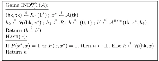
Correctness of PPH schemes.LetP be a predicate on pairs of inputs. We define correctness of a PPHΓ with respect toP via the game CORpphΓ,P(A), which is as follows: It starts by running (hk,tk)← K$ h(1λ) and givestktoA. Then A outputsx, y. The game computesh← H($ hk, x), h0 ← H($ hk, y) and outputs 1 if T(tk, h, h0)6=P(x, y). We say that Γ iscomputationally correct with respect to
P if for all efficientA, Pr[CORpphΓ,P(A) = 1] is a negligible function ofλ.
Security of PPH schemes. We recall a simplified version of the security
definition for PPH that is a weaker version of PPE security defined by Pandey and Rouselakis [35]. The definition is a sort of semantic security for random messages under chosen-plaintext attacks, except that the adversary is restricted from making certain queries.
Game INDpphΓ,P(A):
(hk,tk)← K$ h(1λ) ;x∗ $
← A(tk)
h0 $
← H(hk, x∗) ;h1 $
←R; b← {$ 0,1};b0← A$ Hash(tk, x∗, h
b) Return (b=? b0)
Hash(x):
IfP(x∗, x) = 1 orP(x, x∗) = 1, thenh← ⊥, Elseh← H$ (hk, x) Returnh
Fig. 6: Game INDpphΓ,P(A).
2 Pr[INDpphΓ,P(A) = 1]−1.We say thatΓ is restricted-chosen-input secureif for all efficient adversaries A,AdvpphΓ,P,A(λ)is negligible.
5.2 ORE from PPH
Construction. Let F : K×([n]× {0,1}n) → {0,1}λ be a secure PRF. Let
P(x, y) =1(x=y+ 1) be the predicate that outputs 1 if and only ifx=y+ 1, and letΓ = (Kh,H,T) be a PPH scheme with respect toP. In our construction, we interpret the output ofF as aλ-bit integer, which is also the input domain of the PPHΓ. We define our ORE schemeΠ = (K,E,C) as follows:
– K(1λ, M): On input the security parameter and message space [M], the algorithm chooses a key k uniformly at random for F, and runs the key generation algorithm of the property preserving hash functionΓ.Khto obtain the hash and test keys (hk,tk). It sets ck ← tk, sk ← (k,hk) and outputs (ck,sk).
– E(sk, m): On input the secret key skand a messagem, the algorithm writes the binary representation asm as (b1, . . . , bn), and then for i= 1, . . . , n, it computes:
ui=F(k,(i, b1b2· · ·bi−1||0n−i+1)) +bi mod 2λ, ti=Γ.H(hk, ui). We note thatui is computed by treating the PRF output as a member of {0, . . . ,2λ−1}. Then it chooses a random permutation π : [n] →[n], and setsvi=tπ(i). The algorithm outputsCT= (v1, . . . , vn).
– C(ck,CT1,CT2): on input the public parameter, two ciphertexts CT1,CT2 whereCT1= (v1, . . . , vn),CT2= (v10, . . . , v0n),the algorithm runsΓ.T(tk, vi, vj0) andΓ.T(tk, vi0, vj) for everyi, j∈[n]. If there exists a pair (i∗, j∗) such that Γ.T(tk, vi∗, v0j∗) = 1, then the algorithm outputs 1, meaningm1> m2; else if
there exists a pair (i∗, j∗) such thatΓ.T(tk, v0i∗, vj∗) = 1, then the algorithm
outputs 0, meaningm1< m2; otherwise it outputs⊥, meaningm1=m2.
i∗ ∈ [n] such that ui =u0i+ 1. Therefore correctness of Π is followed by cor-rectness of PPH. We can use the same argument for the case m1 = m2 and m1 < m2. What is more interesting is its simulation based security, as it is the foundation for parameter hiding ORE, formally:
Theorem 14. Assuming F is a secure PRF and Γ is restricted-chosen-input secure, Π isLf-non-adaptively-simulation secure.
Proof. We use a hybrid argument, and define a sequence of hybrid games as follows:
– H−1: Real game REALoreΠ(A);
– H0: Same asH−1, except replacing PRFFk(·) by a truely random function F∗ in the encryption oracle;
– Hi·q+j Depend on a predicateSwitch(i,j)which is define below. IfSwitch(i,j)= 0, thenHi·q+j =Hi·q+j−1, else in procedure of E(mj), u
j
i is replaced by a random string.
From the high level, we establish the proof by showing show that any adjacent hybrids are indistinguishable, and then we construct an efficient simulatorSsuch that the output of Hqn and SIMoreΠ,Lf(A,S) are statistically identical. For the predicate, we say Switchi,j = 1 if ∀k∈[q],msdb(mj, mk)6=i, and 0 otherwise. We note that when Switchi,j = 0, there exists uki such that uji = uki ±1, the relation which can be detected by the test algorithm of PPH(for the i-th bit of mj, we call such a bit a leaky bit), which means we cannot replace it with random string, otherwise adversary can trivially distinguish it. In the following we firstly prove any adjacent objects are computational indistinguishable.
Lemma 15. Assuming Γ is restricted-chosen-input secure, for any k ∈ [qn] Hk−1
comp ≈ Hk.
Proof. Due to the security of PRF, it’s trivial that H−1 comp
≈ H0, and for any k > 0(for ease, k = i∗ ·q+j∗ where i∗ ∈ [n−1], j∗ ∈ [q] ), it suffices to show Hk−1
comp
≈ Hk under the condition Switchi∗,j∗ = 1(Switchi∗,j∗ = 0 implies
Hk−1=Hk). We prove that if there exists adversaryAthat distinguishHk from Hk−1with noticeable advantage, then we can construct a simulatorBwins the restricted-chosen-input game with -negl. Here is the description of B. Firstly it runs INDpphΓ , and sendstk as the comparison key ckto A. After receiving a sequence of plaintext m1, . . . , mq, it picks a random functionF∗(using the lazy sampling technique for instance), setsX∗=F∗(i∗, bj1∗b2j∗· · ·bji∗∗−1||0n−i
∗+1
)+bji∗∗
where bji is thei-th bit ofmj. Then it sends X∗ to its challenger in restricted-chosen-input game and gets back T as the challenge term. To simulate the en-cryption oracle,Bworks as follows:
1. (i0, j0) > (i∗, j∗)(here using a natural order for tuples, (i, j) > (i0, j0) iff iq+j > i0q+j0 ),Bcomputes:
uji00 =F∗(i∗, b
j0 1b
j0 2 · · ·b
j0
i0−1||0n−i 0+1
) +bji00;t
j0
i0 =Γ.H(hk, u
2. (i0, j0)<(i∗, j∗)∩Switchi0,j0 = 0, then same as above, elseuj 0
i0
$
← {0,1}λ, tj0 i0 =
Γ.H(hk, uji00).
3. sets tji∗∗ =T, and ∀j ∈[q], picks a random permutationπj and outputs the
ciphertextsCTj = (t j
πj(1), . . . , t j πj(n)). Finally,Boutputs whateverAoutputs11.
SinceF∗is a random function, Pr[uji00 =X∗±1] is negligible for all (i0, j0)6=
(i∗, j∗), which meansBfails to simulate the encryption oracle with only negligible probability. Besides, whenT =Γ.H(hk, X∗),B properly simulatesHk−1, and if T is random, then B simulates Hk(due to the PRF security, the distribution of Γ.H(hk, r) : r← {0$ ,1}λ is computationally close to a random variable that uniformly sampled from the range ofΓ). Hence, ifAdv(A) is noticeable, then
B’s advantage is also noticeable. ut
In the following, we describe an efficient simulatorS such that the output ofHqn and SIMoreΠ,Lf(A,S) are statistically identical. Roughly speaking, we note
thatSwitchi,j= 1 means thati-th bit ofmjis not a leaky bit, indicating that its value would not affect the leakage profile whp. Hence, it suffices to only simulate the leaky bit of each individual message, which can be extracted byLf, and sets the rest just as random string. Due to the final random permutations,Hqn and SIMoreΠ,Lf(A,S) are statistically identical. Formally:
Description of the simulator. For fixed a message set M = {m1, . . . , mq} (without loss of generality, we assumem1> . . . > mq), the simulatorS is given the leakage information Lf(m1, . . . , mq). S firstly keeps a q×n matrix B and runs a recursive algorithmFillMatrix(1,1, q) to fill in the entries, as follows:
– Ifj =k, then∀i0 ∈[i, n],B[j][i0] =rwherer← {0$ ,1}λ;
– Else, it proceeds as follows:
• searches the smallestj∗∈[j, k] s.t. P(mj, mj∗) =P(mj, mk);
• sets B[j0][i] = r0,∀j0 ∈ [j, j∗−1];B[j0][i] = r0−1,∀j0 ∈ [j∗, k], where r0← {0$ ,1}λ;
• runsFillMatrix(i+ 1, j, j0−1) and FillMatrix(i+ 1, j0, k) recursively. More concretely, our recursive algorithm is to fill in the entries by
FillMatrix(i, j, k), ∀i∈[n], j≤k∈[q]
ThenS runs Γ.Kh(1λ) and gets the keystk,hk, and sets ti,j=Γ.H(hk,B[j][i]), ∀i ∈ [n], j ∈ [q]. Finally, S samples random permutations πj, outputs CTj as CTj= (t
j
πj(1), . . . , t j
πj(n)) We note that the FillMatrix algorithm terminates after at most qn steps as each cell will not be written twice, henceS is an efficient simulator.
Finally we claim thatS properly simulates the relevant games. We first ob-serve that the simulator identifies how many leaked bits (prefixes) there are for 11
the messagesm1, . . . , mq. Recall that if messagesm1, . . . , mqshare the same pre-fix up to the`−1-th bit, and if there exists (the first )i∗such thatmsdb(m1, mi∗) =
msdb(m1, mq), then we can conclude that {m1, . . . , mi∗−1} has 1 on their `-th
bit, and and{mi∗, . . . , mq}has 0 on their`-th bit. This way the`-th bit of these
messages are leaked. The simulator recursively identifies other leaked bits for these two sets. At the end, for each message, how many prefixes whose next bits are leaked will be identified. As this information will also be identified in the hybrid Hqn. So a random permutation (for Hqn and the simulation) will hide these leaked prefixes, except the total number. Thus, our simulation is identical
toHqn, and we establish the entire proof. ut
Now, it is rest to construct a PPH, in section, we give a concrete scheme based on bilinear maps.
6
PPH from Bilinear Maps
We construct a PPH scheme for the predicateP required in our ORE construc-tion. That is, P(x, y) = 1 if and only if x=y+ 1.
We let F : {0,1}λ × {0,1}λ →
Zp be a PRF, where p is a prime to be determined at key generation.
Construction.We now define our PPHΓ = (Kh,H,T).
– Kh(1λ) This algorithm takes the security parameter as input. It samples descriptions of prime-orderp groups G,Gˆ,GT, generatorsg ∈G,ˆg ∈ Gˆ, a
bilinear map e : G×Gˆ → GT. It then chooses k $
← {0,1}λ. It sets the hash keyhk←(k, g,ˆg), the test keytk←(G,Gˆ,GT, e), a description of the bilinear map and groups, and outputs (hk,tk).
– H(hk, x) This algorithm takes as input the hash key hk, an input x, picks two random non-zeror1, r2∈Zp and outputs
H(hk, x) = (gr1, gr1·F(k,x),gˆr2,ˆgr2·F(k,x+1)).
– T(tk, h1, h2) To test two hash values (A1, A2, B1, B2) and (C1, C2, D1, D2), T outputs 1 if
e(A1, D2) =e(A2, D1), and otherwise it outputs 0.
Hence the domainD is{0,1}λ and the rangeR is (
G2,Gˆ2)
Correctness. Correctness reduces to testing if F(k, y+ 1) =F(k, x). Ifx=
y+ 1 then this always holds. If not, then it is easily shown that findingx, ywith this property (and without knowing the key) with non-negligible probability leads to an adversary that contradicts the assumption thatF is a PRF.
Security.We prove that PPH is restricted-chosen-input secure, assuming that