Summary.— An overview of what we know about the climate of the planet Earth up to 5.5 millions of years from now is presented first, with the air temperature in proximity to the surface as the main, and more feasible, parameter to be followed. The behavior of this parameter exhibits a distinct periodicity with more internal fluctuations. This overview prompts us to a description of the physical basis of the climate system, capable of explaining such fluctuations. The system is the star-planet, initially described as a lamp-billiard ball simple system. Astronomical causes affect the distance lamp-billiard ball (star-planet) and the ball (Earth) rotation axis orientation, while astronomical causes affect the intensity of radiation emitted from the lamp (Sun). The complication introduced by the atmosphere is then explained, essentially through the triatomic gas molecules, aerosol and clouds. Atmospheric composition affects incoming solar radiation and outgoing infrared one. The com-partments relevant for climate definition are examined: lithosphere, hydrosphere, cryosphere, biosphere including vegetation and humans. However due to space lim-itations the interactions between the different compartments are not treated here and we restrict ourselves to the treatment of the atmosphere.
1. – Climate and weather
Common sense often leads us to confuse the two terms, and the need for a separate definition of climatology and meteorology is not completely clear to the general public. A simple widely accepted distinction between the two fields is in general based on the different temporal scales that characterize the two.
However, in a scientific approach, the different objectives of the two disciplines imply that a clearer separation both in methodology and in the general theoretical formulations should be made.
Fig. 1. – Meteorological window suggested by Italian Central Office for Meteorology and Climate in 1879 (Tacchini, 1879). In the last decades of the 19th century most of Italian observations were performed in urban environments, in screens located outside a north-facing window of the highest floor of a “meteorological tower”. The purpose of using such towers was to perform observations above the level of the roofs of the surrounding buildings.
The definition of weather is apparently simple. It is the state of the atmospheric system surrounding us at a given moment: clear or cloudy sky, it is raining or not, warm or cold temperatures, humidity, visibility and so on.
Instead, the definition of climate is more complex: in fact, climate isrepresented by the mean state and variations over time, of the same system. Since climatic phenomena have variations that occur on different time scales, from 1 day to 1 million years or more, it is not possible to consider them all together, but it is necessary to focus on a time scale of interest. So we will consider the phenomena that have typical variations on longer time scales as constant, and those that have variations on shorter time scales as rapid and casual fluctuations of the system itself.
Then the problem arises of which meteorological parameter, or combination of param-eters, we should choose as more appropriate to describe the climate. The air temperature in proximity of the surface is the preferred, but others could be chosen even with more scientific value, if data were available from the past as they are for the air temperature. Moreover we can ask ourselves if there are significant space scales which connect different climates, or which time scales (of years, decades, centuries..) should be selected for the arithmetic mean operations. Statistics suggests in fact the arithmetic mean as the most intuitive for analyzing the behavior of climate parameters.
The answer to these questions is obtained by trial and error, and by testing the algorithms and concepts with experience on real data.
In doing so the quality and completeness of data series on which we operate is of great importance.
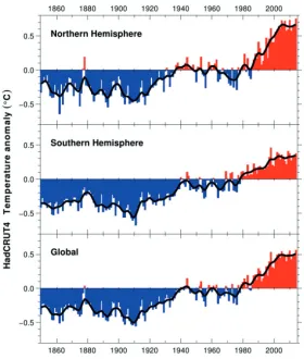
Fig. 2. – Global mean air temperature near to the surface.
2. – Climates in the past
We mentioned the air temperature as the main parameter. It is now measured in many thousands meteorological stations in the world following the rules of WMO, the World Meteorological Organization (two meters above the ground, in a white painted box to shield the direct solar radiation, etc). The reconstruction of reliable historical series of this parameter is not easy at all, since, before strict rules had been dictated, the thermometers were exposed in niches in walls of houses (fig. 1), or exposed to the Sun, shadowed by trees, in countryside locations that have been in decades invaded by large cities peripheries, or sometimes with instruments roughly calibrated. Thanks to specialized teams of scientists we are in conditions, especially in Europe, of having historical series corrected for all possible errors and events, from the beginning of the 19th century and even before, in a few cases.
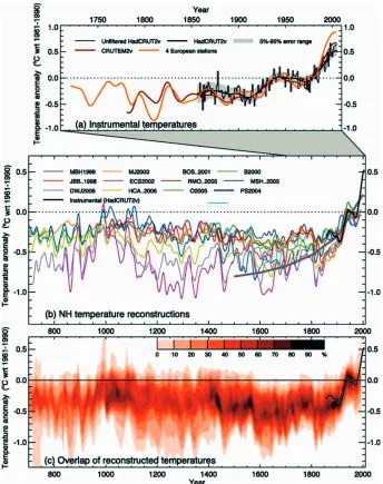
Fig. 3. – Records of Northern Hemisphere temperature variation during the last 1.3 kyr. (a) An-nual mean instrumental temperature records. (b) Reconstructions using multiple climate proxy records and the HadCRUT2v instrumental temperature record in black. (c) Overlap of the published multi-decadal time scale uncertainty ranges of all temperature reconstructions, with temperatures within ±1 standard error (SE) of a reconstruction “scoring” 10%, and regions within the 5 to 95% range “scoring” 5% (the maximum 100% is obtained only for temperatures that fall within±1 SE of all 10 reconstructions). The HadCRUT2v instrumental temperature record is shown in black. All temperatures represent anomalies (◦C) from the 1961 to 1990 mean.
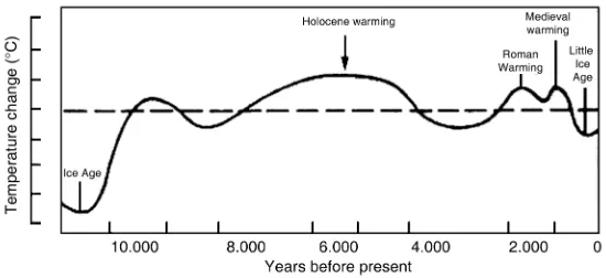
Fig. 4. – Global temperature variations for last 10000 years. Composite of proxies from 1990 IPCC Report.
1920, an increase from 1920 to 1940, then a plateau up to 1980 followed by a remarkable increase from 1980 to 2000. Last 15 years seem to indicate again a plateau, even if 2014 is the hottest year on record.
An increase, globally, of 0.075◦C per decade since 1901 (0.155◦C per decade since 1979) is generally accepted, indicating heating of the Earth atmosphere.
Before proceeding backward to inspect the past climates we need to recall that the historical series of data of temperature in fig. 2 and 3a are the only ones obtained by physical instruments, the thermometers. The three main meteorological instruments were invented (thermometer, by Galileo, barometer, by Torricelli, hygrometer by various experimenters in Italy) or perfected in the first half of the 17th century. Their use in the Accademia del Cimento network of the Granducato di Toscana, first meteorological service in the world, established the 19th of June 1657, soon interrupted ten years later, was then spreading in Europe rather slowly, in academies, observatories and universities. In fig. 3 other “indirect” data are shown. They are called proxy data in the sense that they are not directly giving a measure of the parameter “air temperature close to the surface”, but provide good indications of its behavior.
It is accepted that from 1000 to 1300 the northern hemisphere experienced a warm period (medieval warm period), then a little ice age up to the end of 18th century. If we move to 10000 years from now paleo-climatologists suggest a Holocene maximum of 1 or 2 degrees and an ice age about 12000 years ago, fig. 4.
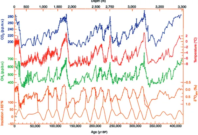
Fig. 5. – Vostok ice core reconstruction of temperature and CO2 and CH4 concentrations over the last 420 kyr.
cycles. Before 400 kyr the character of the ice ages is seen to be somewhat different: interglacial warmth is distinctly less than the four most recent interglacials. However, the interglacial periods before 400 kyr occupied a much larger proportion of each cycle than subsequently. It is also interesting to note how the dominant cycle before 400 kyr is 41 kyr periodicity instead of 100 kyr as in the recent 400 kyr.
Even more instructive is fig. 7: on longer time scales, sediment cores show that the cycles of glacials and interglacials are part of a deepening phase within a prolonged ice age that began with the glaciation of Antarctica approximately 40 million years ago. This deepening phase, and the accompanying cycles, largely began approximately 3 million
Fig. 6. – EPICA expedition ice core reconstruction of temperature and CO2.
Fig. 7. – Five million years of climate change reconstructed with sediment cores.
years ago with the growth of continental ice sheets in the Northern Hemisphere. It is interesting to note the dominant periodicity changes from 41000 yr to 100000 yr. After this look at the past, the problem is to explain these changes in the climate of the planet, which could avoid the two extreme stable cases, the ice ball and the arid water-free “roasted” one.
It is time to present the basic physics behind the system of the couple star-planet in fig. 8.
3. – Back to basics of the climate system
The earth generates heat internally, and this internal source drives plate tectonics, the magnetic field, volcanic eruptions and earthquakes. Some energy also comes in the fast protons and electrons of the solar wind, which cause interesting ionospheric and auroral effects, and there is even a small contribution from cosmic rays, which are mainly very energetic protons and photons. The light from the Moon reaching the Earth is reflected from the Sun, and the light from all stars is negligible. All of these sources of energy are inconsequential compared to sunlight, which extends from 0.15μm in the far ultraviolet to 4μm in the infrared. We can, therefore, safely neglect these inputs and concentrate on the solar input. The total power received on a surface normal to the direction of the Sun outside the atmosphere at the Earth’s distance is 1.94 cal/cm2min or 1367 W/m2. The spectrum is close to a black-body spectrum for 6000 K, crossed by narrow absorption lines due to absorption in the chromosphere of the Sun, the Fraunhofer lines.
We see at the right of fig. 8 the surface of our star, the Sun, with typical rice-grain–like surface, and the dark sunspots. The distance separating the two actors is 150000000 km. The Earth disk is intercepting 1367 W/m2of the Sun radiation and part of it is reflected back into space. If we redistribute on the Earth surface (the Earth is rotating and the disk intercepting radiation is changing continuously) the flux at the top of the atmosphere is 240 W/m2.
The Sun and the Earth emit in two distinct bands of the e.m. spectrum, λmaxT is constant so the Sun emits centered at 6000 K and 0.5μm and the Earth at 288 K and 9μm.
If we assume that the energy absorbed is equal to the one emitted (the two radiative fluxes equal) and no atmosphere present on the planet (billiard ball scheme) we should obtain a temperature of the Earth surface of−18◦C, as shown by the following equation:
S0(1−αp)πrp2=σT44πrp2 → T=4
S0 4
(1−αp)
σ =
4
1367 4
(1−0.3)
5.6710−8= 255 K∼=−18
◦C
WhereS0 is the solar constant,αp is the planetary albedo,σ is the Boltzmann con-stant,rpis the Earth radius and T the planetary emission temperature.
However the atmosphere is there, transparent enough to visible (Sun) radiation, but with great ability to absorb infrared radiation. By introducing the effect of the atmo-sphere we have a termTAin equation, and a flux balance is obtained as in fig. 9, leading to a surface temperature of about +15◦C. The atmosphere is nearly transparent to short-wave radiation, but is relatively opaque to long-wave radiation, except in a few “windows” of transmission. Therefore, it acts like the glass of a greenhouse, absorbing and emitting long-wave radiation according to its temperature.
We need to explain why the gaseous envelop plays such important role. In fig. 10, below the black-body curves of solar and terrestrial radiation the curve of absorp-tion/transmissivity is shown vs. wavelength. The bands of O2, O3 H2O, CH4 are in-dicated combined, while separately in the following fig. 11. One observation comes im-mediately: those gases are negligible contributors to the total mixture of atmospheric
Fig. 9. – Schematic sketches of the greenhouse effect.
gases, but have a fundamental role in the radiative transfer. They play such role because they are composed of three or more atoms.
While the visible light can make it through the surface the infrared radiation from the surface has only one, and not complete “window” towards the outer space, between 8 and 13μm.
Fig. 11. – Infrared absorption spectra for various atmospheric gases.
In summary the atmosphere is transparent enough to visible radiation but has a great ability in absorbing infrared radiation. In fig. 11 the behavior of individual gases shows the important role of water vapor, N2O, methane, CO2 and O3. The consequence is that only a small part of the radiation emitted by the surface of the Earth and by the lower layers of the atmosphere can leave definitively the planet while most is absorbed by the above listed tri-atomic gases. The clear sky atmospheric gases re-emits towards the surface, but even more effective in re-emitting is the cloud cover in its lower part. This leads to an entrapment of infrared radiation and such entrapment is rather improperly called greenhouse effect. It is just the natural greenhouse effect which leads to a new surface radiation balance which is schematically shown in fig. 9.
The major constituents of the atmosphere, the diatomic gases nitrogen and oxygen, and the 1% of argon, do not interact with electromagnetic radiation in the long-wave
so carbon dioxide will have a much smaller effect than water vapour. It should be realized that both the greenhouse effect and carbon dioxide are essential to life on Earth.
The water vapour absorbs long-wavelength radiation very strongly, and will be nearly opaque to it, so that it is emitted and absorbed continuously. The radiation will be emitted at the surface at a temperature of 288 K, but will be emitted into space at 217 K, as required for equilibrium. Water vapour is by far the most important contributor to this process, by means of its large concentration and strong rotational spectrum.
The question now is posed, after our excursion in the past which has shown climate changes and the basics of the physics of climate, which are the causes of these changes? Two main reasons: the lamp and the billiard ball scheme, we can suppose that the distance lamp ball changes and the intensity of the lamp changes. The first cause is called an astronomical cause and the second an astrophysical cause. They combine in changing the amount of radiation reaching the top of the atmosphere.
We will then recognize an additional cause, the change of atmospheric composition, through the processes of radiative transfer mentioned above. This is adding a complica-tion which needs an explanacomplica-tion.
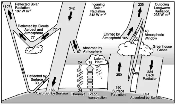
All the above considerations can be quantified in the scheme of fig. 12 which indicates the contributions in Wm−2to the steady state energy budget of the Earth. The numbers represent energy in units of Watt m−2 the figures are rough estimates but show the relative contributions.
4. – Causes of climate changes
Fig. 12. – Schematic diagram of the global radiation budget in the climate system.
Fig. 13. – Sunspot number observations. Since ca. 1749, continuous monthly averages of sunspot activity have been available and are shown here as reported by the Solar Influences Data Analysis Center, World Data Center for the Sunspot Index, at the Royal Observatory of Belgium.
As astrophysical processes we indicate the processes which change the radiation emit-ted by the Sun: sunspots, which have a cycle, the solar wind, the coronal mass ejections and the flares.
The Sun is the source of energy that warms the Earth, therefore it is reasonable to expect a close relationship between the variation in the flow of that energy and our planet’s climate.
There is observational evidence that relates particular climatic events of the past with different rates of energy received. An example is the so-called Little Ice Age, an
ability can justify only a variation of the magnitude of 0.1 degrees between maxima and minima.
4.2. Compartments and interactions. – The compartments of climate systems are essentially five and processes relevant to climate systems take place inside each of them or between adjacent compartments.
– Atmosphere: the gaseous component of the climate system is the most rapidly changing over time.
– Cryosphere: includes glaciers, snowfields, ocean ices.
– Lithosphere: orographic structure of the Earth, which changes very slowly over time.
– Hydrosphere: oceans, seas, rivers, lakes.
– Biosphere: flora, fauna, human activity.
Both atmosphere and hydrosphere are responsible of the latitudinal redistribution of the uneven solar heating through their respective circulations. The major difference is that atmospheric circulation is clearly separated into the two hemispheres, while the ocean one is a unique conveyor belt for the whole planet.
4.3.Changes in atmospheric composition and climate. – We have shown that a cause of climate change is related to the variation in atmospheric composition. These are originated by nature or by humans. Among the natural causes leading to changes in atmospheric composition we mention those originated in the interaction between the climate system components, such as the oceans interactions, or atmosphere-biosphere interactions.
In fact important exchanges take place between ocean and atmosphere in water vapor, momentum and CO2. Same fluxes of CO2 and water vapor are exchanged between vegetation, or the whole biosphere, and the atmosphere.
of solids and liquids in deserts and oceans surfaces, and gas to particle conversion and combustion are important source mechanisms. Many anthropic activities imitate nature in these mechanisms for generating aerosols, while greenhouse gases such as CO2, SO2 are generated by combustions and CH4 by breeding of animals. The reduction of forest areas for agriculture or other uses leads to variations in albedo and consequently leads to climate changes.
An important interaction of atmosphere and ocean affecting climate but not related to changes in composition is the so-called El Ni˜no and La Ni˜na, whereas the surface warm areas of the Pacific ocean move between eastern coasts of Australia to coasts of south America and vice versa with important consequences on weather in both hemispheres
In normal non–El-Ni˜no conditions.
– Trade winds blow westwards.
– Sea surface is about 1/2 meters higher at Indonesia than at Ecuador.
– SST is about 8 degrees C lower in the east supporting marine ecosystems fisheries.
– West Pacific regions are wet, while the east Pacific is relatively dry.
While during El Ni˜no
– Depression of the thermocline in the eastern Pacific and elevation of the thermocline in the west.
– Rise in SST and a drastic decline in primary productivity.
– Rainfall follows the warm water eastward, flooding in Peru and drought in Indonesia and Australia.
– Trade winds relax in the western Pacific.
– Large changes in the global atmospheric circulation.
5. – Aerosols, clouds, water cycle and climate
Aerosols, the liquid and solid particles suspended in the air influence climate through direct and indirect effects.
Direct effects are due to scattering and absorption of solar and terrestrial radiation. Indirect effects are linked to the aerosol role as cloud condensation nuclei and ice-forming nuclei, which determine the microphysical characteristics of clouds and then influencing their radiative properties and lifetime.
In fig. 12 we notice visually the role of clouds in the radiative transfer. More than that is shown there, we can say that clouds are at the core of the climate problem and until their presence is quantitatively represented with their true effects in climate models we cannot pretend of forecasting climate. At most we can produce scenarios with a very low degree of reliability.
Clouds increase the albedo and generate their own greenhouse effect. It is estimated that clouds increase on average the outgoing flux of solar radiation by−48 Wm−2 and decrease the outgoing flux of infrared radiation by−31 Wm−2 on a global scale. Thus the effect of clouds on the net radiative flux is−17 Wm−2, with a global mean effect of atmospheric cooling.
How does this effect take place? The radiative fluxes are affected when a cloud is present above and below and inside. Above and below because of temperature, aerosol and water vapor profiles, modulated by surface properties. Inside because of the macro-physical structure (optical thickness, vertical and horizontal inhomogeneities) and micro-physical characteristics (cloud particles size distribution, shape, phase of cloud particles)
In table I we show the importance of cloud type on the radiation budget.
There is not here the possibility to enter into the details of computations. However it is noteworthy to say in a context of a school the great challenge for physicist to contribute to solve the climate problem through a correct description of scattering of e.m. radiation by cloud particles
Many problems remain unsolved. We mention the followings:
– Microphysical properties (phase, size distribution) are often fixed parameters in GCM.
– The numerical solution of single scattering.
– Single scattering treatment is not always realistic and multiple scattering approach is sometimes necessary.
– Complexity of non plane parallel clouds with highly inhomogeneous structures (3D effects) are taken into account neither in cloud microphysical retrievals nor in GCM.
– Optical properties of non-spherically shaped ice particles.
Concluding, clouds exert a strong impact on climate through radiative energy redis-tribution via the scattering and absorption of radiation, playing also an important role in the hydrological cycle.
They constitute the main source of uncertainty in global climate models, arising principally from two types of problems related to cloud-climate interactions:
– definition of the cloud radiative properties in climate models, through a knowledge of cloud morphology and microphysical characteristics,
– and simulation of the behavior of clouds in a changing climate, along with their feedback mechanisms.
As a consequence the water cycle of which clouds and precipitation are the visible leg in the atmosphere stands as the guide of the climate system.
Further readings
Hartmann D. L.,Global Physical Climatology (Academic Press, New York) 1994.
Peixoto J. P.andOort A. H.,Physics of Climate(American Institute of Physics) 1992.