i
ELASTIC SCATTERING OF ELECTRON BY BARIUM ATOM USING DISTORTED WAVE METHOD
KAGO JAMES NDUNGU (B. Ed (Sc.)) I56/CE/28347/2013
A thesis submitted in partial fulfillment of the requirements for the award of the degree of Master of Science (Physics) in the School of Pure and Applied Sciences of Kenyatta University.
DECLARATION
This thesis is my original work and has not been presented for award of a degree in any other University.
KAGO JAMES NDUNGU ……… ……….. (I56/CE/28347/2013) signature date
We confirm that the candidate, under our supervision, carried out the work reported in this thesis.
PROF. CHANDRA SINGH ……… ………. Signature date Department of Physics
Kenyatta University
PROF. JOHN OKUMU ………. …..….………. Signature date
ACKNOWLEDGEMENTS
My deepest gratitude and appreciation goes to my supervisor, Prof. C.S. Singh for his unwavering support. Without whose patience and guidance none of this would
have happened on schedule, or at all. His experience in the field of atomic collisions was exceedingly beneficial in the success of this work. Thanks to my second supervisor, Prof. J. Okumu for taking an interest in my work. I thank the department of physics, Kenyatta University, for admitting me to the master degree program. I extend my appreciation to my colleague Martin Kimani for his helpful discussions we held and his supportive encouragements. Am highly indebted to my parents Mr. and Mrs. Kago for having given me the education foundation and the desire to aim
for the best in life.
TABLE OF CONTENTS
DECLARATION ... ii
DEDICATION ... iii
ACKNOWLEDGEMENTS ... iv
TABLE OF CONTENTS ... v
LIST OF TABLES ... vii
LIST OF FIGURES ... viii
ABBREVIATIONS ... ix
ABSTRACT ... x
CHAPTER 1 ... 1
INTRODUCTION ... 1
1.1 Background Of The Study ... 1
1.2 Statement Of The Problem... 4
1.3 Objectives ... 4
1.3.1 General Objective ... 4
1.3.2 Specific Objectives ... 4
1.4 Rationale For The Study ... 5
CHAPTER 2 ... 6
LITERATURE REVIEW ... 6
2.1 Experimental Studies On Electron-Barium Scattering ... 6
2.2 Theoretical Calculations ... 6
2.3 Summary Of Review ... 9
CHAPTER 3 ... 10
THEORETICAL BACKGROUND OF APPROXIMATION METHODS ... 10
3.1 Introduction To Theoretical Methods ... 10
3.2 Quantum Mechanical Methods ... 11
3.2.1 The Born Approximation ... 11
3.2.2 Coulomb –Projected Born (Cpb) Approximation ... 12
3.2.3 The R-Matrix Method ... 12
3.2.5 Optical Potential Method ... 13
3.2.6 The Distorted Wave Methods (Dwm)... 14
3.2.6.1 Distorted Wave Formula Using Two-Potential Scattering Model .... 15
CHAPTER 4 ... 19
MATERIALS AND METHODS ... 19
4.1 Application Of Distorted Wave Formula To Electron- Barium Scattering ... 19
4.2 The Distorted Wave ... 23
4.3 Differential Cross Section (Dcs) And Integral Cross Section (Ics) ... 24
4.4 Distortion Potential ... 25
4.4.1 Introduction ... 25
4.4.2 Evaluation Of Static Potential ... 25
4.5 Atomic Wave Function ... 31
4.6 Computer Code ... 36
CHAPTER 5 ... 37
RESULTS AND DISCUSSION ... 37
5.1 Introduction ... 37
5.2 Differential Cross Sections ... 37
5.3 Integral Cross Section ... 52
CHAPTER 6 ... 55
CONCLUSIONS AND RECOMMENDATIONS ... 55
6.1 Introduction ... 55
6.2 Conclusions ... 55
6.3 Recommendations ... 56
LIST OF TABLES
Table 4.1: 1s, 2s, 3s, 4s, 5s and 6s radial atomic wave functions for ground state of barium (mclean and mclean, 1981). ... 33 Table 5.1: Present dwm differential cross section (in 𝒂𝟎𝟐/𝒔𝒓) for elastic
scattering of electron by barium atom, at different impact energies. ... 38 Table 5.3: DWM integral cross sections (in 𝒂𝟎𝟐) for elastic scattering of
electron by barium atom. ... 53
LIST OF FIGURES
Figure 1.1: A schematic diagram for atomic scattering ... 2 Figure 5.1: Differential cross section for elastic scattering of electron by barium
atom at 10 ev incident energy.)... 39 Figure 5.2: Differential cross sections for elastic scattering of electron by barium
atom at 15 ev incident energy. ... 40 Figure 5.3: Differential cross section of elastic scattering of electron by barium atom at 20 ev incident energy. ... 41 Figure 5.4: Differential cross sections of elastic scattering of electron by barium
atom at 30 ev incident energy.. ... 42 Figure 5.5: Differential cross sections of elastic scattering of electron by barium
atom at 40 ev incident energy. ... 43 Figure 5.6: Differential cross sections of elastic scattering of electron by barium
atom at 60 ev incident energy.. ... 44 Figure 5.7: Differential cross sections of elastic scattering of electron by barium
atom at 80 ev incident energy.. ... 45 Figure 5.8: Differential cross section of elastic scattering of electron by barium atom at 100 ev incident energy.. ... 46 Figure 5.9: Differential cross sections of elastic scattering of electron by barium
atom at 200 ev incident energy. ... 47 Figure 5.10: Integral cross sections for elastic scattering of electron by barium
ABBREVIATIONS
CC2 Two-State Close Coupling
CCC Convergent Close Coupling
CCC115 One hundred and fifteen – state Convergent Close Coupling
CPB Coulomb Projected Born
DCS Differential Cross Section
DHF Dirac-Hartree-Fock
DWM Distorted Wave Method
DWBA Distorted Wave Born Approximation
DWBA1 e−H inelastic scattering computer program
eV electron Volt
FBA First Born Approximation
HFS Hartree-Fock-Slater
ICS Integral Cross Section
ABSTRACT
CHAPTER 1 INTRODUCTION 1.1 Background of the study
Theory of atomic collision is crucial for theoretical as well as experimental studies in atomic physics, in particular cross sections of e- - Ba scattering are needed for modeling the behavior of Ba vapor lasers, discharge lamps, plasma switches and various ionosphere where Ba has often been used as trace element for diagnostic purpose (Fursa et al., 1999). On the academic side benchmark laboratory cross section are needed for testing various theoretical approximation and calculation methods hoping to predict these cross sections (Fursa et al., 1999).
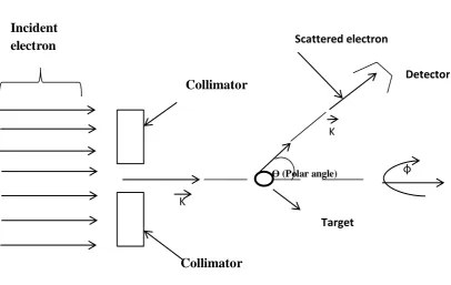
In the study of atomic collisions a beam of free projectile is made to interact with the target and a detector record the scattered particles in the asymptotic region. A schematic diagram of the experimental arrangement is shown in figure 1.1. After the interaction between the projectile and target, their respective energy configuration may be conserved, this is known as elastic scattering. If exchange of energy between projectile and target occurs, resulting in target excitation, ionization, annihilation or positronium formation, this is an inelastic scattering (Ali and Soding, 1988).
Electron-atom scattering yields differential cross section (DCS) results. The differential cross section is a measure of probability that electrons will be scattered in a given direction specified by the polar and azimuthal angles θ and ϕ
Figure 1.1: A schematic diagram for atomic scattering
In quantum mechanics scattering is described as a probability event. We can only calculate the probability that the particles got scattered into a certain direction, not precise angles of scattering. The aim of electron –atom scattering is to model as accurately as possible the behavior of the electron –atom system in the interaction region, such knowledge is used in the interpretation and prediction of results from electron-atom scattering experiments.
In the early days of atomic scattering experiments, only total cross sections were measured and most theoretical approaches gave results in reasonable agreement with the experimental data, at least for higher energies (Madison and Bartschart, 1996). During this time the first Born approximation (FBA) became very popular due to its ease of calculation. In 1960’s experimental techniques were improved and differential cross section measurement started to be reported, thus experiments
Ɵ (Polar angle)
Collimator K
Incident electron s
Collimator Detector
ɸ K
Scattered electron
revealed that the FBA was valid only for small angles and further that the angular range over which the FBA was valid decreased with energy of incident projectile. The reason that the FBA gave good results for the total cross section was that its major contribution came from very small scattering angles where the FBA was reliable. For application which are sensitive to large angle differential cross section, theoretical approach superior to FBA were required. As a result a number of theoretical methods have been developed for calculation of cross section including the distorted wave Born approximation DWBA (Joachain, 1975), the close-coupling method (McCarthy and Weigold, 1995) and R-matrix method (Burke and Berrington, 1993).
1.2 Statement of the problem
Over the last three decades several theoretical DCS and ICS results for elastic scattering of e-- Ba scattering at intermediate energies have been reported. The first calculated result were obtained using two state close-coupling (CC2) method (Fabrikant, 1980), later Fursa and Bray (1999) used convergent close coupling method (CCC-115). Also there has been result from relativistic polarized orbital method (Szmytkowski and Sienkiewzc, 1994). Miloshevsky et al. (2000) used phase theory to compute these cross sections. However, no known results on elastic scattering of electron by barium have been reported using distorted wave method (DWM), so it was interesting to see how it works.
1.3 Objectives
1.3.1 General objective
The main objective was to study the elastic scattering of electron by barium atom using the distorted wave method.
1.3.2 Specific objectives
i. To formulate the distorted wave method applied to electron - barium scattering.
ii. To modify the computer program DWBA1 for the calculation.
iv. To compare the result with other available theoretical and experimental results and draw conclusions on the suitability of the DWM for this calculation.
1.4 Rationale for the study
Jensen et al. (1978) used beam-beam configuration experiment technique to measure cross sections for elastic scattering of electron by barium at impact energies of 20, 30, 40, 50, 60, 80 and 100 eV in the 3° to 130° angular range. However, these results are in serious disagreements with the work of Szmytkowski and Sienkiewicz (1994) where relativistic polarized orbital method was used to calculate the cross sections for electron scattering from barium at impact energies of 15, 20, 30, 40, 60, 80 and 100 eV.
CHAPTER 2
LITERATURE REVIEW 2.1 Experimental studies on electron-barium scattering
There are various data available from experimental results data on e--Ba elastic scattering at intermediate energies. Jensen et al. (1978) used beam-beam configuration experiment to study the elastic scattering of electron from barium at impact energies of 20, 30, 40, 50, 60, 80 and 100 eV in the 3° to 130° angular range. Wang et al. (1994) measured the elastic cross section for impact energies of 5, 10, 15 and 20 eV at angular range of 3° to 130°. Extrapolations to larger angles were performed using theoretical calculations. When the ICS and momentum transfer cross sections were compared with other experimental and theoretical results, good agreement was found at small angles but significant deviation was found at large angles. Trajmar et al. (1999) were interested in measurement of collision and coherence parameters as well as cross sections associated with an atomic ensemble prepared with an arbitrary in –plane laser geometry and linear polarization (with respect to collision frame) or equivalently with any magnetic sublevel superposition which were obtained at 20 eV impact energy at 10° and 20° scattering angles.
2.2 Theoretical calculations
experimental results of Jensen et al. (1978) and Wang et al. (1994) at impact energies of 20 and 30 eV. However, this agreement is only at small angle but not at intermediate scattering angles.
Fursa and Bray (1999) used convergent close coupling (CCC-115) to calculate DCS and ICS at impact energies of 15, 20, 30, 50, 60, 80 and 100 eV. The calculation of barium structure was performed in the non-relativistic LS coupling scheme. For the Ba structure the model of two valence structure electrons above an inert Hartree-Fock core was used. Configuration-Interaction (CI) expansion (for valence electrons) was used to calculate target wave function. These theoretical results are in good agreement with experimental data of Jensen et al. (1978) and Wang et al. (1994). However, these results are in poor agreement with calculations of Szmytkowski and Sienkiewicz (1994) up to 60 eV but relatively good agreement is found at 80 and 100 eV.
Miloshevsky et al. (2000) used phase theory to calculate DCS and ICS for e-- Ba elastic scattering at impact energies of 15, 20, 30, 40, 60 and 100 eV. The calculation were performed with Hartree-Fock-Slater (HFS) approximation taking into account the polarization effect but excluding exchanges and spin interaction between incident and atomic electron. When their results are compared with experimental data of Jensen et al. (1978) and Wang et al. (1994) satisfactory agreement is seen.
Adibzadeh and Theodosiou (2004) have given a comprehensive result for differential, total and momentum transfer cross section and Sherman function for impact energies of 15, 20, 30, 40 and 60 eV. These results were obtained using standard method of partial wave-expansion in potential scattering and the partial wave phase shift which were obtained by solving the time-independent Dirac- equation. When compared with other experimental and theoretical results, DCS are in good agreement with the results of Wang et al. (1994) and CCC (115) results of Fursa and Bray (1999) but differ from results of Jensen et al. (1978). The ICS are in good agreement with experimental results but are found to be higher than those of CCC (115) results of Fursa and Bray (1999) at intermediate energies.
Kumar et al. (1994) employed semi-relativistic approach to compute the DCS, ICS, spin polarization P and spin polarization parameters T and U for electron scattering from barium atom in the energy range 2-300 eV. The projectile target interaction was represented both by real potential and complex potential in the solution of Dirac equation for scattered electrons. The real optical potential included the static, a parameter free correlation polarization and a modified semi classical exchange potentials. The complex optical potential was constructed by adding a model absorption potential as its imaginary part to the real optical potential.
2.3 Summary of review
From the above it is clear that so far no study can claim to be in perfect agreement with other results at intermediate and high energy region. It is on this basis that a study of electron-barium elastic scattering using distorted wave method has been conducted. This study employs static potential of barium atom at ground state as the distortion potential. The wave functions that have been used are Roothan-Hartree-Fock (RHF) double zeta wave functions (McLean and McLean, 1981). The results obtained have been compared with available experimental and theoretical results.
CHAPTER 3
THEORETICAL BACKGROUND OF APPROXIMATION METHODS
3.1 Introduction to theoretical methods
Due to the demand for the atomic collision data set in various fields of physics, various experimental techniques and theoretical approaches have been developed in order to get reliable data sets for atomic collision processes. Theoretical approaches to scattering are either classified as quantum mechanical approaches or semi-classical approaches. Quantum approaches which use the principle of quantum mechanics exclusively are further classified as perturbative methods and close coupling methods. The latter is based on close coupling techniques that expand trial wave functions. Some of the close coupling methods include convergent close coupling and the R-matrix methods. Perturbative methods are based on Born series expansion and examples include First Born approximation, eikonal Born series, Coulomb Projected Born approximation, many body theory and the Distorted wave series.
3.2 Quantum mechanical methods
3.2.1 The Born approximation
In the Born series expansion, the scattering amplitude is written as
𝑓 = − 1
4𝜋⟨𝜓𝑘𝑓|𝑈 + 𝑈𝐺0
+𝑈 + 𝑈𝐺
0+𝑈𝐺0+𝑈+. … |𝜓𝑘𝑖⟩ (3.1)
Here 𝜓𝑘𝑓 is the product final plane wave 𝑒𝑖𝑘𝑓.𝑟 of the projectile and the final target wave function 𝜑𝑓.
𝜓𝑘𝑖 is the product of the initial plane wave 𝑒𝑖𝑘𝑖.𝑟 of the incident particle and the initial atomic wave function 𝜑𝑖. U is the interaction potential and the function 𝐺0+ is outgoing Green’s function given as
𝐺0+(𝑘, 𝑟, 𝑟′) = 1 4𝜋
𝑒𝑖𝑘|𝑟−𝑟′|
|𝑟−𝑟′| (3.2)
The first term in series (3.2.1) is the first Born approximation to scattering amplitude and is given as
𝑓𝐵1 = − 1
4𝜋⟨𝜓𝑘𝑓|𝑈|𝜓𝑘𝑖⟩ (3.3)
3.2.2 Coulomb –Projected Born (CPB) approximation
The Coulomb-projected Born approximation consists basically of modifying the usual Born approximation by taking an explicit account of the Coulomb interaction between the projectile and the nucleus. The final state plane wave in the Born approximation is replaced by a Coulomb wave in CPB method. Different ways of taking this coulomb interaction into account has led to different CPB methods, for example CPB approximation by Geltman, (1971), Generalized CPB approximation by Stauffer and Morgan, (1975) and a variable charge CPB approximation by Schaub-shaver and Stauffer, (1980). These approximations give better results than Born approximation results and are useful in describing collisions of electrons and ions with target atoms and ions (Joachain, 1975).
3.2.3 The R-Matrix method
in an appropriately chosen basis in the internal region and cross section calculated by solving the asymptotic problem in external region (Burke et al., 1971).
3.2.4 Convergent close coupling (CCC) method
This method is suitable for elastic and inelastic scattering at lower impact energies of the projectile. The CCC method relies on close coupling formalism for solving the coupled equation without approximations. The convergence is tested by including the ever increasing set of states in the close coupling formalism. The target states are obtained by diagonalising the target Hamiltonian in an orthogonal Laguerre basis which ensures that completeness is approached as the basis size increases. The CCC treats both the discrete and continuum parts of the target space through the close coupling formalism; this allows the validity of the CCC method to be independent of the projectile energy or transition of interest (Fursa and Bray, 1999).
3.2.5 Optical potential method
3.2.6 The Distorted wave methods (DWM)
Distorted wave methods were introduced because the Born approximation failed to give accurate account of differential cross section for low impact energies and large scattering angles. In the distorted wave approximation, the incident electron is taken to be elastically scattered by the initial state atomic potential. If the scattering is through direct process, the incident electron makes a transition to a state in which it is being elastically scattered by the final state atomic potential. If the scattering of electron is through the exchange process, the incident electron is captured into a bound state of the atom, while one of the initially bound electrons is ejected. In this case, the transition between the initial and final state is calculated by perturbation method. It is suitable for calculation of differential cross section for electron scattering by atoms at intermediate and high incident energies (Itikawa, 1986).
3.2.6.1 Distorted wave formula using two-potential scattering model
In this section, the distorted wave method is discussed within the frame work of a two potential formalism. The total Hamiltonian for the projectile is written as
𝐻 = 𝐻0+ 𝑉 (3.4)
where V is the interaction potential between the projectile and the target. 𝐻0 is the unperturbed Hamiltonian of the target atom and the non-interacting projectile. In the two potential formalism the interaction potential is broken in a physically meaningful way in two parts: one which is treated exactly (𝑈𝑠), and the other which is handled in an approximate way (𝑊𝑠) ( Joachain, 1975). That is,
𝑉𝑠 = 𝑊𝑠+ 𝑈𝑠 (3.5)
where s=i or s= f for initial and final states respectively. It is assumed that the equation
(𝐻0 + 𝑈)𝜒± = 𝐸𝜒± (3.6)
can be solved exactly. 𝜒 is the product of target wave function and projectile wave function within the interaction region (distorted wave) and + (-) refers to the outgoing (incoming) wave boundary conditions.
The transition matrix elements for any scattering problem is given as,
𝑇𝑖𝑓 = ⟨𝜙𝑓|𝑉𝑓|Ψ𝑖+⟩ (3.7)
where 𝜙𝑓 is the product of final target wave function and final plane wave of the projectile in the asymptotic region and Ψ𝑖+ is the total wave function of the system
𝐻Ψ𝑖+ = 𝐸Ψ𝑖+ (3.8)
Making use of equation (3.2.5), equation (3.2.7) can be written as
𝑇𝑖𝑓 = ⟨𝜙𝑓|𝑈𝑠+ 𝑊𝑠|Ψ𝑖+⟩ (3.9)
Since
|𝜒𝑓−⟩ = |𝜙𝑓⟩ + 1
𝐸𝑓−𝐻𝑓−𝑖𝜖𝑈𝑓|𝜙𝑓
⟩ (3.10)
where 𝐻𝑓 = 𝐻0+ 𝑈𝑓 and this Hamiltonian, it can written as
⟨𝜙𝑓| = ⟨𝜒𝑓−| − ⟨𝜙 𝑓|𝑈𝑓
1
𝐸𝑓−𝐻𝑓+𝑖𝜖 (3.11)
Expanding equation (3.9) and making use of equation (3.11), the transition matrix elements can be written as,
𝑇𝑖𝑓 = ⟨𝜙𝑓|𝑈𝑓|Ψ𝑖+⟩ + ⟨𝜒𝑓−|𝑊𝑓|Ψ𝑖+⟩ − ⟨𝜙𝑓|𝑈𝑓 1
𝐸𝑓−𝐻𝑓+𝑖𝜖𝑊𝑓|Ψ𝑖
+⟩ (3.12)
The third term of (3.12) can be transformed using the relation
|Ψ𝑖+⟩ = |𝜙𝑖⟩ + 1
𝐸𝑖−𝐻+𝑖𝜖𝑉𝑖|𝜙𝑖
⟩ (3.13)
where 𝜙𝑖is the product of the initial atomic wave function and the initial plane wave
for the projectile, as (on the energy shell E=𝐸𝑖 = 𝐸𝑓)
⟨𝜙𝑓|𝑈𝑓 1
𝐸𝑓−𝐻𝑓+𝑖𝜖𝑊𝑓|Ψ𝑖
+⟩ = ⟨𝜙
𝑓|𝑈𝑓 1
𝐸−𝐻𝑓+𝑖𝜖𝑊𝑓|𝜙𝑖⟩
+⟨𝜙𝑓|𝑈𝑓 1 𝐸−𝐻𝑓+𝑖𝜖𝑊𝑓
1
And further making use of equation (3.11), equation (3.14) can be written as,
⟨𝜙𝑓|𝑈𝑓 1
𝐸𝑓−𝐻𝑓+𝑖𝜖𝑊𝑓|Ψ𝑖
+⟩ = ⟨𝜒
𝑓−|𝑊𝑓|𝜙𝑖⟩ − ⟨𝜙𝑓|𝑊𝑓|𝜙𝑖⟩
+ ⟨𝜙𝑓|𝑈𝑓 1
𝐸−𝐻𝑓+𝑖𝜖𝑊𝑓
1
𝐸−𝐻+𝑖𝜖𝑉𝑖|𝜙𝑖⟩ (3.15)
Making use of operator identity
1 𝐵(𝐵 − 𝐴) 1 𝐴 = 1 𝐴− 1 𝐵
where A=𝐸 − 𝐻 +i𝜖 and B=𝐸 − 𝐻𝑓+ 𝑖𝜖 and recalling that 𝐻 − 𝐻𝑓 = 𝑊𝑓, then
⟨𝜙𝑓|𝑈𝑓 1 𝐸−𝐻𝑓+𝑖𝜖𝑊𝑓 1 𝐸−𝐻+𝑖𝜖𝑉𝑖|𝜙𝑖⟩ = ⟨𝜙𝑓|𝑈𝑓 1 𝐸−𝐻+𝑖𝜖𝑉𝑖|𝜙𝑖⟩ − ⟨𝜙𝑓|𝑈𝑓 1
𝐸−𝐻𝑓+𝑖𝜖𝑉𝑖|𝜙𝑖⟩ (3.16)
Using equations (3.11) and (3.13), equation (3.16) can be written as
⟨𝜙𝑓|𝑈𝑓 1 𝐸−𝐻𝑓+𝑖𝜖𝑊𝑓 1 𝐸−𝐻+𝑖𝜖𝑉𝑖|𝜙𝑖⟩ = ⟨𝜙𝑓|𝑈𝑓|Ψ𝑖 +⟩ − ⟨𝜙 𝑓|𝑈𝑓|𝜙𝑖⟩ −⟨𝜒𝑓−|𝑉
𝑖|𝜙𝑖⟩ + ⟨𝜙𝑓|𝑉𝑖|𝜙𝑖⟩ (3.17)
Substituting equations (3.15) and (3.17) in equation (3.12), we get
𝑇𝑖𝑓 = ⟨𝜙𝑓|𝑈𝑓|Ψ𝑖+⟩ + ⟨𝜒𝑓−|𝑊𝑓|Ψ𝑖+⟩ − ⟨𝜒𝑓−|𝑊𝑓|𝜙𝑖⟩ + ⟨𝜙𝑓|𝑊𝑓|𝜙𝑖⟩ − ⟨𝜙𝑓|𝑈𝑓|Ψ𝑖+⟩ +
⟨𝜙𝑓|𝑈𝑓|𝜙𝑖⟩ + ⟨𝜒𝑓−|𝑉𝑖|𝜙𝑖⟩ − ⟨𝜙𝑓|𝑉𝑖|𝜙𝑖⟩ (3.18)
Using the fact that on the energy shell
Equation (3.18) can be written as
𝑇𝑖𝑓 = ⟨𝜒𝑓−|𝑉𝑖 − 𝑊𝑓|𝜙𝑖⟩ + ⟨𝜒𝑓−|𝑊𝑓|Ψ𝑖+⟩ (3.19)
This is the two potential formula of Gellmann and Goldberger (Joachain, 1975).
When 𝑉𝑖 = 𝑉𝑓 = 𝑉 and 𝑊𝑓 = 𝑉 − 𝑈𝑓 are taken, the T-matrix can be written as
𝑇𝑖𝑓 = ⟨𝜒𝑓−|𝑈𝑓|𝜙𝑖⟩ + ⟨𝜒𝑓−|𝑊𝑓|Ψ𝑖+⟩ (3.20)
CHAPTER 4
MATERIALS AND METHODS
4.1 Application of distorted wave formula to electron- barium scattering
Total Hamiltonian, H, for electron –barium scattering is given as,
H=Ha+T+V (4.1)
where Ha is the Hamiltonian of the isolated atom, T the Hamiltonian for the projectile electron (kinetic energy operator) and V is the interaction between the projectile and atom, given as (in atomic units)
𝑉 =−𝑍
𝑟0 + ∑
1 𝑟0𝑖
𝑧
𝑖=1 (4.2)
where z is the atomic number of the atom, 𝑟0 is the position coordinate of the projectile electron from the nucleus of the target and 𝑟0𝑖 is the position coordinate of the projectile relative to ith atomic electron.
The initial state full scattering wave function Ψi+, representing the projectile-atom is a solution of Schrödinger equation.
(H − E)Ψi+ = 0 (4.3)
where the (+) superscript indicates the outgoing wave boundary conditions.
(when the total wave function Ψ𝑖+ is written in the antisymmetrized form and 𝜒 is written as the product of the projectile and target wave functions, equation (3.20) obtained in the previous chapter takes this form)
𝑇𝑖𝑓 = (𝑁 + 1)〈𝜒𝑓−(0)𝜓𝑓(1, … . . , 𝑁)|𝑉 − 𝑈𝑓|𝐴𝛹𝑖+(0, … … , 𝑁)〉
+⟨𝜒𝑓−(0)𝜓
𝑓(1, … … . , 𝑁)|𝑈𝑓|𝜓𝑖(1, . . , 𝑁)𝛽𝑖(0)⟩ (4.4)
where𝛽𝑖 is the initial plane wave given as,
𝛽𝑖 = 𝑒𝑥𝑝(𝑖𝑘. 𝑟𝑜) (4.5)
𝜓𝑖 and 𝜓𝑓 are the initial and final wave functions of the barium atom respectively. A
is the antisymmetrization operator for the electron-atom system which may be expressed as,
𝐴 = 1
𝑁+1(1 − ∑ 𝑃𝑖0
𝑁
𝑖=1 ) (4.6)
where Pi0 is the operator that exchanges the 𝑖𝑡ℎ atomic electron with incident
electron (denoted by 0).
𝜒𝑓− is the distorted wave (distorted by distortion potential 𝑈𝑓) satisfying incoming wave boundary condition and is a solution of the wave equation
(∇02+ 𝑈
𝑓− 𝑘𝑓2)𝜒𝑓− = 0 (4.7)
𝑘𝑓 is the final state wave vector of projectile electron (𝑘𝑓2 gives kinetic energy (in
𝑈𝑓 is an arbitrary potential (which is generally chosen as a static potential of the target ) for distortion of the final projectile electron wavefunction.
The value of Ψ𝔦+ in (4.3) cannot be evaluated exactly and hence need for more approximation. Its value is expressed in terms of product of initial state distorted wave 𝜒𝔦+ times an initial atomic wave function 𝜓𝑖. That is,
Ψ𝑖+(0, 1, … 𝑁) = 𝜓𝑖(1, 2, … . . 𝑁)𝜒𝑖+(0) (4.8)
where 𝜒𝑖+ is the distorted wave function representing the projectile electron in the initial state and is solution to wave equation
(∇02+ 𝑈
𝑖 − 𝑘𝑖2)𝜒𝑖+ = 0 (4.9)
The Lippmann-Schwinger solution for Ψi+ in terms of 𝜒
𝑖+ is given by
Ψ𝑖+= [1 + 𝐺+(𝑉 − 𝑈
𝑖)]𝜓𝑖𝜒𝑖+ (4.10)
where 𝐺+ is the Green’s function having the form
𝐺+ = (𝐸 − 𝐻 + 𝔦𝜀)-1 (4.11)
Introducing a third arbitrary potential U and hence the Green’s function in the form
𝑔+ = (𝐸 − 𝐻
𝑎 − 𝑇 − 𝑈 + 𝑖𝜂)−1 (4.12)
associated with potential, the full Green’s function G+ may be expressed in terms of the distorted Green’s function as
G+=g+ + G+ (V-U) g+ (4.13)
G+ = g++G+ (V-U) g++G+ (V-U) g+ (V-U) g+ (4.14)
If the Lippmann-Schwinger solution (4.10) is substituted in (4.3) along with Green’s function expansion (4.1.14) we get
𝑇𝔦𝑓=T1+T2+T3+………….. (4.15)
where
𝑇1= (𝑁 + 1)⟨𝜒𝑓−(0)𝜓
𝑓(1, . . 𝑁)|𝑉 − 𝑈𝑓|𝐴𝜓𝑖(1, . . 𝑁)𝜒𝑖+(0)⟩
+⟨𝜒𝑓−(0)𝜓𝑓(1, … 𝑁)|𝑈𝑓|𝜓𝑖(1, … , 𝑁)𝛽𝑖(0)⟩ (4.16)
𝑇2 = (𝑁 + 1)⟨𝜒𝑓−(0)𝜓
𝑓(1, … . 𝑁)
|𝑉 − 𝑈𝑖)𝐴𝑔+(𝑉 − 𝑈
𝑖)|𝜓𝑖(1, … 𝑁)𝜒𝑖+(0)⟩ (4.17)
and
𝑇3 = (𝑁 + 1)⟨𝜒𝑓−(0)𝜓𝑓(1, … 𝑁)|𝑉 − 𝑈𝑓)
𝐴𝑔+(𝑉 − 𝑈𝑖)𝑔+(𝑉 − 𝑈𝑖)|𝜓𝑖(1, … 𝑁)𝜒𝑖+(0)⟩ (4.18)
Equation (4.15) is the distorted wave series for the T-matrix while (4.16) is the first order distorted wave approximation (DWBA1).
Within the above frame work (DWBA1) one is able to calculate the expressions for direct and exchange- matrices.
𝑇𝑖𝑓 = 𝑇𝑑− 𝑇𝑒𝑥 (4.19)
where direct matrix
𝑇𝑑 = ⟨𝜒𝑓−(0)ψ𝑖(1, 2)|𝑈𝑓|ψ𝑖(1, 2)𝛽𝑖(0)⟩ (4.20)
and exchange matrix
𝑇𝑒𝑥 = −⟨𝜒
𝑓−(0)ψ𝑖(1, 2)|𝑉 − 𝑈𝑓|ψ𝑖(0, 2)𝜒𝑖+(1) + 𝜓𝑖(1, 0)𝜒𝑖+(2)⟩ (4.21)
Since ψ𝑖 = ψ𝑓 the first term in equation (4.6) vanishes for direct scattering. When
making calculations we are going to neglect the term associated with 𝑈𝑓 in 𝑇𝑒𝑥,
assuming that the overlap integral between the bound state and distorted wave will be negligible because of oscillatory nature of distorted wave. The 𝑇𝑒𝑥 then takes the
form
𝑇𝑒𝑥 = −⟨𝜒𝑓−(0)𝜓𝑓(1, 2)|𝑉|𝜓𝑖(0, 2)𝜒𝑖+(1) + 𝜓𝑖(1, 0)𝜒𝑖+(2)⟩ (4.22)
4.2 The distorted wave The distorted wave χ𝑖+ and 𝜒
𝑓− for projectile in the initial and final states are
expanded in terms of partial waves (Singh, 2005), as
|𝜒𝑖+⟩ = √2 𝜋 1 𝑘𝑖𝑟∑ 𝑖 𝑙𝑖 𝑙𝑖𝑚𝑖 𝜒𝑙𝑖(𝑘𝑖, 𝑟)𝑌𝑙𝑖𝑚𝑖(𝒓̂ )𝑌𝑙∗𝑖𝑚𝑖(𝒌̂
𝑖) (4.23)
and
|𝜒𝑓−⟩ = √2 𝜋 1 𝑘𝑓𝑟 ∑ 𝑖𝑙𝑓𝜒 𝑙𝑓 ∗ 𝑙𝑓𝑚𝑓 (𝑘𝑓, 𝑟)𝑌𝑙𝑓𝑚𝑓(𝒓̂ )𝑌𝑙∗𝑓𝑚𝑓(𝒌̂
where 𝑌𝑙𝑚 are spherical harmonics and 𝑟̂ and 𝑘̂ are unit vectors denoting the direction of r and k. In the expansion of 𝜒𝑓− the complex conjugate of radial part is taken so that it satisfies the incoming wave boundary condition.
Substituting (4.23) and (4.24) into equations (4.7) and (4.9) respectively we find that the radial distorted waves are solutions of the following equation,
(𝑑2 𝑑𝑟2−
𝑙𝑠(𝑙𝑠+1)
𝑟2 − 𝑈𝑠(𝑟) + 𝑘𝑠
2) 𝜒
𝑙(𝑟) = 0 (4.25)
with s=i for initial state and s=f for the final state distorted waves. In asymptotic region, they satisfy the boundary condition,
𝑙𝑖𝑚𝑟→∞𝜒𝑙𝑠(𝑘𝑠, 𝑟) = 𝑗𝑙𝑠 + 𝐵𝑙𝑠(−𝜂𝑙𝑠 + 𝑖𝑗𝑙𝑠) (4.26)
where 𝑗𝑙 and 𝜂𝑙 are regular and irregular Ricatti-Bessel functions and 𝐵𝑙 is given as,
𝐵𝑙 = exp (𝑖𝛿𝑙) sin 𝛿𝑙 (4.27)
where 𝛿𝑙 is elastic scattering phase shift.
4.3 Differential cross section (DCS) and integral cross section (ICS)
The radial distorted wave equations (4.2.3) for initial and final states was solved using Numerov method (Madison and Bartschart, 1996) and differential cross section was obtained using the relation,
𝑑𝜎
𝑑Ω = 4𝜋
4 𝑘𝑓
𝑘𝑖(|𝑇
𝑑− 𝑇𝑒𝑥|2) (4.28)
𝜎 = ∫𝑑𝜎𝑑Ω𝑑Ω = 2𝜋 ∫0𝜋𝑑Ω𝑑𝜎sin 𝜃𝑑𝜃 (4.29)
4.4 Distortion potential
4.4.1 Introduction
Since elastic scattering is being considered, both the initial and final distortion potential were taken as static potential of a barium atom in the initial state, that is,
𝑈𝑖 = 𝑈𝑓 = ⟨ψ𝑖|𝑉|ψ𝑖⟩ (4.30)
where 𝑈𝑖 and 𝑈𝑓 are initial and final distortion potentials respectively.
4.4.2 Evaluation of static potential
The mathematical formulation of static potential is generally expressed as
𝑈𝑠 = ⟨𝜓𝑠|𝑉|𝜓𝑠⟩ (4.31)
where 𝜓𝑠 is target wave function, s=i or f for initial or final state respectively and V is the interaction between the projectile and the target. For the target state we have used the Roothan –Hartree-fock wave functions compiled by McLean and McLean (1981).
Since we are considering a target with two electrons,
𝜓𝑠 = 𝜓0(𝑟1)𝜓0(𝑟2) (4.32)
and
𝑉 = 2
𝑟01+
2 𝑟02−
4
𝑟0 (in Rydberg units ) (4.33)
𝑈𝑠 = ⟨𝜓0(𝑟1)𝜓0(𝑟2)| 2 𝑟01+
2 𝑟02−
4
𝑟0|𝜓0(𝑟1)𝜓0(𝑟2)⟩ (4.34)
Equation (4.34) simplifies to
𝑈𝑠 = 2 ⟨𝜓0(𝑟1)| 2
𝑟01|𝜓0(𝑟1)⟩ − ⟨𝜓0(𝑟1)|
4
𝑟01|𝜓0(𝑟1)⟩ (4.35)
Equation (4.35) can now be written as,
𝑈𝑠 = 4 ⟨𝜓0| 1
𝑟01−
1
𝑟0|𝜓0⟩ (4.36)
The wave function 𝜓𝑠 is summed up over slater type orbitals of the basis set as,
|𝜓0⟩ = ∑ 𝐶𝑛 𝑛|ϕ𝑛⟩ (4.37)
and
⟨𝜓0| = ∑ 𝐶𝑛′ 𝑛∗′⟨ϕ𝑛′| (4.38)
The values of 𝐶𝑛 represent the expansion coefficient and ϕ𝑛 are the slater type orbitals of the basis set. Using equations (4.37) and (4.38) in equation (4.36) we can now write the distortion potential as,
𝑈𝑠 = 4 ∑ ∑ 𝐶𝑛𝐶𝑛∗ ′ ⟨𝜙𝑛′| 1
𝑟01 −
1 𝑟0|𝜙𝑛⟩
𝑛′
𝑛 (4.39)
But 1
𝑟01 can be expanded in terms of the spherical harmonics as,
1
𝑟01 = ∑
∑ 4𝜋
2𝑙+1 𝑟<𝑙
𝑟>𝑙+1
+𝑙 𝑚=−𝑙 ∞
where 𝑟<(𝑟>) is lesser (greater) between 𝑟0 and 𝑟1. Since in our elastic scattering calculation the state involved is the s state, using equation (4.39) and (4.40) the static potential can be written as,
𝑈𝑠 = 4 ∑ ∑ 𝐶𝑛 𝑛′ 𝑛𝐶𝑛′⟨𝜙𝑛′| 1
𝑟>−
1
𝑟0|𝜙𝑛⟩ (4.41)
From McLean and McLean (1981) tables, the slater type orbitals are expressed as product of radial function and spherical harmonics 𝑌𝑙,𝑚 and are given as,
𝜙𝑛 = 𝑁𝑛𝑟𝜇𝑛−1exp (−𝜉𝑟)𝑌
𝑙,𝑚(𝑟̂) (4.42)
where 𝜇𝑛 is the principle quantum number of the 𝑛𝑡ℎ orbital of the basis set, 𝜉 is
orbital exponent and the normalization factor 𝑁𝑛 of the orbital is given as,
𝑁𝑛 = ((2𝜇𝑛)!)−12∗ (2𝜉)𝜇𝑛+ 1
2 (4.43)
Substituting the value of the wave function given by equation (4.42) and replacing the bra and the ket notation with standard integrals, the static potential can be fully expanded as,
𝑈𝑠 = 4 ∑ ∑ 𝐶𝑛𝐶𝑛∗′𝑁𝑛𝑁𝑛∗′∫ 𝑟1
𝜇𝑛+𝜇𝑛′
(1 𝑟1−
1 𝑟0)
∞ 𝑟0
𝑛′𝑙′𝑚′
𝑛𝑙𝑚
exp(−[𝜉𝑛+ 𝜉𝑛′]𝑟1) 𝑑𝑟1𝑌𝑙𝑚(𝑟𝑜)𝑌
𝑙′𝑚′
∗ (𝑟
1) (4.44)
In getting equation (4.44) from (4.41), partial integration of radial component is used such that from the radial distance 0 to 𝑟0, 𝑟0 considered to be greater than 𝑟1
Therefore, the distortion potential in effect reduces to,
𝑈𝑠 = 4 ∑ ∑ 𝐶𝑛 𝑛′ 𝑛𝐶𝑛∗′𝑁𝑛𝑁𝑛∗′
∫ 𝑟1𝜇𝑛+𝜇𝑛′(1
𝑟1−
1
𝑟0) exp(−[𝜉𝑛+ 𝜉𝑛
′]𝑟1) 𝑑𝑟1
∞
𝑟0 (4.45)
In this study the integral was evaluated analytically to obtain the exact static potential which has been used as the distortion potentials. It can be easily seen that the static potential is summation of all the elements of a nx𝑛, matrix. The analytical solution of each element of equation (4.45) varies in form depending on the sum of principle quantum numbers, 𝜇𝑛 and 𝜇𝑛′. This sum varies between 2 and 12 for the problem that was solved as follows
For 𝑟2
∫ 𝑒−𝑘𝑟(1
𝑟−
1 𝑟0)𝑟
2𝑑𝑟 ∞
𝑟0
=−𝑒−𝑘𝑟0[1
𝑘2+
2 𝑘3𝑟
0] (4.46)
For 𝑟3
∫ 𝑒−𝑘𝑟(1
𝑟−
1 𝑟0)𝑟
3 ∞
𝑟0
𝑑𝑟
=−𝑒−𝑘𝑟0[𝑟0
𝑘2+
4
𝑘3+
6
𝑘4𝑟0] (4.47)
∫ 𝑒−𝑘𝑟(1
𝑟−
1 𝑟0)𝑟
4𝑑𝑟 ∞
𝑟0
= −𝑒−𝑘𝑟0[𝑟0 2
𝑘2+
6𝑟0
𝑘3 +
18
𝑘4+
24 𝑘5𝑟
0]
(4.48)
For 𝑟5
∫ 𝑒−𝑘𝑟 ∞ 𝑟0 (1 𝑟− 1 𝑟0)𝑟
5𝑑𝑟
= −𝑒−𝑘𝑟0[𝑟0 3
𝑘2+
8𝑟02
𝑘3 +
36𝑟0
𝑘4 +
96
𝑘5+
120 𝑘6𝑟
0] (4.49) For 𝑟6
∫ 𝑒−𝑘𝑟(1
𝑟−
1 𝑟0)𝑟
6𝑑𝑟 ∞
𝑟0
= −𝑒−𝑘𝑟0[𝑟0 4
𝑘2+
10𝑟03
𝑘3 +
60𝑟02
𝑘4 +
120𝑟0
𝑘5 +
600
𝑘6 +
720
𝑘7𝑟0] (4.50)
For 𝑟7
∫ 𝑒−𝑘𝑟 ∞ 𝑟0 (1 𝑟− 1 𝑟0)𝑟
7𝑑𝑟
= −𝑒−𝑘𝑟0[𝑟0 5
𝑘2+
12𝑟04
𝑘3 +
90𝑟03
𝑘4 +
480𝑟02
𝑘5 +
18000𝑟0
𝑘6 +
4320
𝑘7 +
5040 𝑘8𝑟
0] (4.51)
For 𝑟8
∫ 𝑒−𝑘𝑟 ∞ 𝑟0 (1 𝑟− 1 𝑟0)𝑟
= −𝑒−𝑘𝑟0[𝑟0 6
𝑘2+
14𝑟05
𝑘3 +
126𝑟04
𝑘4 +
840𝑟03
𝑘5 +
4200𝑟02
𝑘6 +
15120𝑟0
𝑘7 +
35280
𝑘8 +
40320 𝑘9𝑟
0 ] (4.52) For 𝑟9
∫ 𝑒−𝑘𝑟(1
𝑟−
1 𝑟0) 𝑟
9𝑑𝑟 ∞
𝑟0
= −𝑒−𝑘𝑟0[ 𝑟0 7
𝑘2+
16𝑟06
𝑘3 +
168𝑟05
𝑘4 +
1344𝑟04
𝑘5 +
8400𝑟03
𝑘6 +
40320𝑟02
𝑘7 +
141120𝑟0
𝑘8 +
322560
𝑘9 +
362880
𝑘10𝑟0 ] (4.53)
For 𝑟10
∫ 𝑒−𝑘𝑟 ∞ 𝑟0 (1 𝑟− 1 𝑟0)𝑟
10𝑑𝑟
= −𝑒−𝑘𝑟0[𝑟0 8
𝑘2+
18𝑟07
𝑘3 +
216𝑟06
𝑘4 +
2016𝑟05
𝑘5 +
15120𝑟04
𝑘6 +
90720𝑟03
𝑘7 +
423360𝑟02
𝑘8 +
1451520𝑟0
𝑘9 +
3265920
𝑘10 +
3628800
𝑘11 ] (4.54)
For 𝑟11
∫ 𝑒−𝑘𝑟(1
𝑟−
1 𝑟0)𝑟
11 ∞
𝑟0
𝑑𝑟
= −𝑒−𝑘𝑟0[𝑟0 9
𝑘2+
20𝑟08
𝑘3 +
270𝑟07
𝑘4 +
2880𝑟06
𝑘5 +
25200𝑟05
𝑘6 +
181440𝑟04
𝑘7 +
1058400𝑟03
𝑘8 +
4838400𝑟02
𝑘9 +
16329600𝑟0
𝑘10 +
36288000
𝑘11 +
39916800 𝑘12𝑟
For 𝑟12
∫ 𝑒−𝑘𝑟(1
𝑟−
1 𝑟0)𝑟
12 ∞
𝑟0
= −𝑒−𝑘𝑟0[𝑟0 10
𝑘2 +
22𝑟09
𝑘3 +
330𝑟08
𝑘4 +
3960𝑟07
𝑘5 +
39600𝑟06
𝑘6 +
332640𝑟05
𝑘7 +
2328480𝑟04
𝑘8 +
13305600𝑟03
𝑘9 +
59875200𝑟02
𝑘10 +
199584000𝑟0
𝑘11 +
439084800
𝑘12 +
479001600 𝑘13𝑟
0 ] (4.56)
4.5 Atomic wave function
The atomic wave functions used in evaluation of the direct and exchange transition matrices outlined above are the Roothan-Hatree-Fock double zeta functions given in the McLean and McLean (1981) tables. They are based on the Roothan-Hartree-Fock (RHF) expansion technique. The double zeta function is an approximate RHF function in which a given electron orbital is described by two slater functions. In the above model, the total wave function Ψ is a slater determinant and is given by,
Ψ = 𝐴(Φ1(1)… … … . . Φ𝑛(𝑛)) (4.57)
A is the anti-symmetrizing operator, n is the total number of electrons, and
Φ1(1)… . . Φ𝑛(𝑛) are spin orbitals. The spin orbitals are a product of spin function and
an orbital function. The orbitals are assumed to be orthogonal to each other, thus the same hold for spin orbitals. The orbitals are characterized by an index 𝜂, which indicates the symmetry species and it corresponds to quantum number I, an index 𝛾
refers to the 𝑖𝑡ℎ orbital of symmetry 𝜂 also characterizes the orbitals. The orbitals Φ𝑖𝜂𝛾 is expanded in terms of the basis functions according to,
Φ𝑖𝜂𝛾 = ∑ 𝜙𝑝 𝑝𝜂𝛾𝐶𝑖𝜂𝑝 (4.58)
where p refers to the 𝑝𝑡ℎ basis function of symmetry 𝜂. The expansion coefficients
depend on i, 𝜂 and p but not on 𝛾. The basis functions 𝜙𝑝𝜂𝛾 are slater orbitals with integer quantum numbers, namely,
𝜙𝑝𝜂𝛾(𝑟, 𝜃, 𝜙) = 𝑅𝑛𝑝(𝑟)𝑌𝜂𝛾(𝜃, 𝜙) (4.59)
where
𝑅𝜂𝑝 = [(2𝜇𝜂𝑝)!]−
1 2 (2𝜉
𝜂𝑝) 𝜇𝜂𝑝+12
𝑟𝜇𝜂𝑝−1𝑒𝜉𝜂𝑝𝑟 (4.60)
And 𝑌𝜂𝛾(𝜃, 𝜙) are normalized spherical harmonics in complex form. It is noted that
𝜇𝜂𝑝 ≥ 𝜂 + 1 and that the exponent 𝜉𝜂𝑝 is chosen so as to give the best energy.
The single electron wave function given in equation (4.32) is constructed using the table of coefficient and exponent provided in the atomic data tables of McLean and McLean (1981).
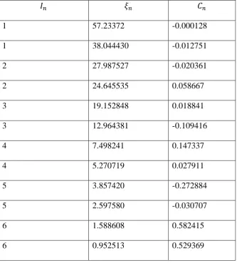
The table 4.1 below shows 𝐼𝑛, 𝜉𝑛 and 𝐶𝑛 denoting the orbitals, zetas and coefficient respectively for the 1𝑠22𝑠22𝑝63𝑠23𝑝63𝑑104𝑠24𝑝64𝑑105𝑠25𝑝66𝑠2 ground state of
Table 4.1: 1s, 2s, 3s, 4s, 5s and 6s radial atomic wave functions for ground state of barium (McLean and McLean, 1981).
𝐼𝑛 𝜉𝑛 𝐶𝑛
1 57.23372 -0.000128
1 38.044430 -0.012751
2 27.987527 -0.020361
2 24.645535 0.058667
3 19.152848 0.018841
3 12.964381 -0.109416
4 7.498241 0.147337
4 5.270719 0.027911
5 3.857420 -0.272884
5 2.597580 -0.030707
6 1.588608 0.582415
6 0.952513 0.529369
The atomic wave function is given by
Φ6𝑠 = −0.000128Φ1− 0.012751Φ2− 0.020361Φ3+ 0.058667Φ4+
0.018841Φ5 −0.109416Φ6+ 0.147337Φ7+ 0.027911Φ8− 0.272884Φ9−
0.030707Φ10+ 0.582415Φ11+ 0.529369Φ12 (4.61)
where
Φ1 = 𝑁1𝑟0exp (−57.233372𝑟)𝑌
Φ2 = 𝑁2𝑟0exp (−38.044430𝑟)𝑌
00(𝜃, 𝜙) (4.63)
Φ3 = 𝑁3𝑟1exp (−27.987527𝑟)𝑌
00(𝜃, 𝜙) (4.64)
Φ4 = 𝑁4𝑟1exp (−24.645535𝑟)𝑌00(𝜃, 𝜙) (4.65)
Φ5 = 𝑁5𝑟2exp (−19.152848𝑟)𝑌
00(𝜃, 𝜙) (4.66)
Φ6 = 𝑁6𝑟2exp (−12.964381𝑟)𝑌
00(𝜃, 𝜙) (4.67)
Φ7 = 𝑁7𝑟3exp (−7.498241𝑟)𝑌
00(𝜃, 𝜙) (4.68)
Φ8 = 𝑁8𝑟3exp (−5.270719𝑟)𝑌
00(𝜃, 𝜙) (4.69)
Φ9 = 𝑁9𝑟4exp (−3.857420𝑟)𝑌
00(𝜃, 𝜙) (4.70)
Φ10 = 𝑁10exp (−2.597580𝑟)𝑌00(𝜃, 𝜙) (4.71)
Φ11 = 𝑁11exp (−1.588608𝑟)𝑌00(𝜃, 𝜙) (4.72)
Φ12 = 𝑁12exp (−0.952513𝑟)𝑌00(𝜃, 𝜙) (4.73)
where 𝑁1… … … . . 𝑁12 are normalization factors given by,
𝑁𝑖 = ((2𝑛)!)−
1 2(2𝜉
𝑛)𝑛+
1
2 (4.74)
where n and 𝜉𝑛 are orbital and zeta respectively, given in table 4.1 above.
𝑁1 = ((2 ∗ 1)!)−
1
2(2 ∗ 57.233372)1+12 (4.75)
𝑁2 = ((2 ∗ 1)!)−
1
𝑁3 = ((2 ∗ 2)!)−
1
2(2 ∗ 27.987527)2+
1
2 (4.77)
𝑁4 = ((2 ∗ 2)!)
−12
(2 ∗ 24.645535)2+
1
2 (4.78)
𝑁5 = ((2 ∗ 3)!)−
1
2(2 ∗ 19.152848)3+12 (4.79)
𝑁6 = ((2 ∗ 3)!)−
1
2(2 ∗ 12.964381)3+12 (4.80)
𝑁7 = ((2 ∗ 4)!)−
1
2(2 ∗ 7.498241)4+12 (4.81)
𝑁8 = ((2 ∗ 4)!)
−1
2(2 ∗ 5.270719)4+
1
2 (4.82)
𝑁9= ((2 ∗ 5)!)−
1
2(2 ∗ 3.857420)5+
1
2 (4.83)
𝑁10 = ((2 ∗ 5)!)−
1
2(2 ∗ 2.597580)5+12 (4.84)
𝑁11 = ((2 ∗ 6)!)−
1
2(2 ∗ 1.588608)6+12 (4.85)
𝑁12 = ((2 ∗ 6)!)−
1
2(2 ∗ 0.952513)6+
1
2 (4.86)
4.6 Computer code
CHAPTER 5
RESULTS AND DISCUSSION
5.1 Introduction
In section 5.2 the DWM differential cross section results for elastic scattering of electron by barium atom obtained in this study are presented. The results are compared with available experimental and theoretical results. In section 5.3 the DWM integral cross sections are presented and compared with earlier results. The DCS which has dimensions of area per unit solid angle are in 𝑎02/𝑠𝑟 units and ICS
are in 𝑎02 units (𝑎0 and sr are Borh radius and steradian respectively)
5.2 Differential cross sections
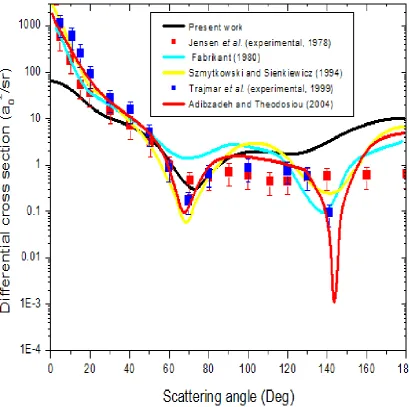
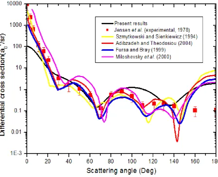
In this study the differential cross section (DCS) for elastic scattering of electron by barium atom have been calculated at 10, 15, 20, 30, 40, 60, 80, 100 and 200 eV for scattering angles from 𝜃 = 0° to 𝜃 = 180°using distorted wave method. To test the
reliability of the present model, the present results have been compared with experimental and theoretical data. Results of such comparisons for elastic scattering of electron from barium atom are presented in figures 5.1-5.9. The present results are listed in table 5.1.
Table 5.1: Present DWM differential cross section (in 𝒂𝟎𝟐/𝒔𝒓) for elastic
scattering of electron by barium atom, at different impact energies. Energy
Angle(θ°)
10 eV 15 eV 20 eV 30 eV 40 eV 60 eV 80 eV 100 eV 200 eV
0 23.78 91.3 72.9 65.11 69.49 84.2 98.27 110.3 148.12
10 103.29 72.82 55.27 44.14 42.77 44.38 45.58 45.64 38.82 20 60.69 39.41 27.78 18.42 14.96 12.0 10.44 9.35 6.1
30 25.98 17.76 13.9 10.16 8.32 6.34 5.17 4.35 2.22
40 8.72 8.32 8.15 7.04 5.95 4.36 3.34 2.66 1.12
50 3.22 4.20 4.37 3.81 3.13 2.15 1.57 1.22 0.5
60 3.1 2.58 1.95 1.28 0.90 0.53 0.39 0.32 0.18
70 4.85 2.5 1.11 0.27 0.14 0.14 0.17 0.18 0.13
80 6.42 2.82 1.22 0.61 0.68 0.77 0.69 0.58 0.23
90 6.53 2.54 1.33 1.42 1.74 1.74 1.40 1.07 0.31
100 4.94 1.44 0.99 1.94 2.50 2.36 1.78 1.27 0.26
110 2.56 0.24 0.51 1.93 2.53 2.27 1.61 1.07 0.13
120 1.02 0.27 0.74 1.72 2.00 1.59 1.03 0.63 0.02
130 1.80 2.67 2.61 1.94 1.41 0.74 0.41 0.25 0.10
140 5.55 7.80 6.50 3.07 1.26 0.16 0.084 0.20 0.46
150 11.64 14.9 11.94 5.12 1.77 0.066 0.21 0.56 1.05
160 18.38 22.25 17.62 7.56 2.72 0.38 0.65 1.16 1.73
170 23.61 27.79 21.95 9.55 3.62 0.79 1.12 1.72 2.25
those of Fursa and Bray (1999) appearing at 60°and 110° but deeper than the present ones. Adibzadeh and Theodosiou (2004) have three minima.
At 15 eV, figure 5.2 shows that the present results for the differential cross sections are in some qualitative agreement with experimental results of Wang et al. (1994). Both results have two minima. However, the present calculated result first minimum is shallow and the second one has been shifted towards the left as compared with measured results of Wang et al. (1994). This may be attributed to the approximation method used. The present results are also seen to be in qualitative agreement with calculated convergent close coupling results of Fursa and Bray (1999) and potential scattering results of Adibzadeh and Theodosiou (2004)). Quantitatively the present results are higher for angles greater than 120° compared to measured results of
Wang et al. (1994) as well as the calculated results Fursa and Bray (1999) and Adibzadeh and Theodosiou (2004)). This is due to the fact that 15 eV is considered to be low impact energy and DWM is not expected to give good results at low energy. The good qualitative agreement indicates that the distortion potentials in this study are appropriate.
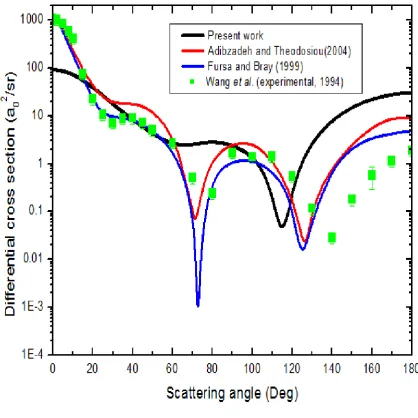
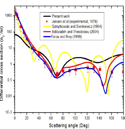
In figure 5.3 we have presented the present DCS results along with experimental and theoretical results at 20 eV. The experimental measurement of Wang et al. (1994) shows two minima in contrast to the observation of Jensen et al. (1978), which shows three minima. The present results are in better qualitative agreement up to
120° with measured results of Wang et al. (1994) than those of Jensen et al.
results have two minima at 70° and 110° compared to those of Wang et al. (1994) appearing at 30°, 80°and 140°. The one appearing at 30° is very shallow but those
at 80° and 140° are deeper. The calculated results of Fursa and Bray (1999),
Adibzadeh and Theodosiou (2004) and Szmytkowski and Sienkiewicz (1994) have also two minima but minima in the results of Szmytkowski and Sienkiewicz (1994) and Adibzadeh and Theodosiou (2004) are deeper compared with the present results. This is because of the potentials used and wave functions employed which are different from the one used in the present study.
Figure 5.4 for impact energy at 30 eV shows, for angle between 10° to 120° the
present results are in satisfactory agreement with the measured results of Jensen et al. (1978) and Trajmar et al. (1999) and two state close coupling (CC2) results of Fabrikant (1980), relativistic polarized orbital results of Szmytkowski and Sienkiewicz (1994) and potential scattering results of Adibzadeh and Theodosiou (2004). The minima at 70° almost coincide in position and depth with the measured
results. According to Miloshevsky et al. (2000) both the depth and positions of minimum in DCS have significant physical importance since they reflect the structural information of the targets. This agreement signifies the accuracy of the present approximation method. For angle greater than 120° the present DCS values
are slightly higher than those of Jensen et al. (1978). This is because within this range (130°− 180°) their results were obtained by, probably incorrect extrapolation (Szmytkowski and Sienkiewicz, 1994).
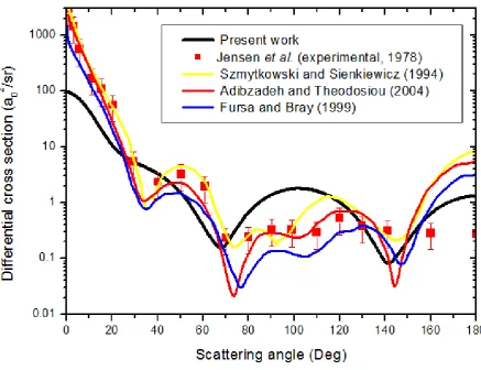
Adibzadeh and Theodosiou (2004) for angle between 200 to 800. The minima at 70° coincide in position and depth with the measured results of Jensen et al. (1978).
For angles greater than 800 the present DCS values are higher than those of
measured results of Jensen et al. (1978) and theoretical results of Fursa and Bray (1999) and Adibzadeh and Theodosiou (2004). The present results are in poor agreement with calculated results of Szmytkowski and Sienkiewicz (1994) having the oscillatory behavior which is not seen in any of the calculated and experimental results. The minima at 140° is shallow compared to the other theoretical results.
This might be attributed to static potentials used which are different from the one used in the present study.
At impact energy 60 eV, figure 5.6, the present results have two minima, a shallow first minima at 70° and a slightly deeper at 150°. The present results are in good
quantitative agreement with measured results of Jensen et al. (1978) and all the available theoretical results except that of Szmytkowski and Sienkiewicz (1994) which is too oscillatory. All the experimental and theoretical results including the present one show two minima except the one due to Szmytkowski and Sienkiewicz (1994).
In figure 5.7 at 80 eV the present results are in good both quantitative and qualitative agreement with measured results of Jensen et al. (1978). The present results have two minima as the measured results. The first minimum at about 70° coincide in
position and depth with the measured one. The present results predict deeper second minimum at 140° compared to the minimum at 110° that is predicted by the
calculated results of Fursa and Bray (1999), Adibzadeh and Theodosiou (2004) and Szmytkowski and Sienkiewicz (1994) since they predict more than two minima. But the differential cross section values of the present results are in the same range as other calculations.
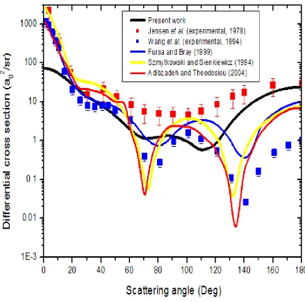
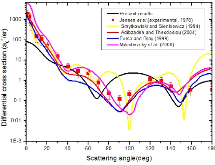
From figure 5.8 at 100 eV, it is seen that the present results from 20° are in better
agreement with measured results of Jensen et al. (1978) compared to the calculated results of Fursa and Bray (1999), Adibzadeh and Theodosiou (2004), Szmytkowski and Sienkiewicz (1994) and Miloshevsky et al. (2000). The present results have two minima as the measured results by Jensen et al. (1978). The position and depth of the first minima almost coincide with the measured results of Jensen et al. (1978) while the second minima have same depth as the experimental results but the position is shifted. The present results have good quantitative agreement (results are in same range) but poor qualitative agreement with the available theoretical results. This is because while the present results have two minima the other calculated results have more than two minima. It is encouraging to note that the present model is capable of reproducing DCS that are in good accord with the measured results.
At 200 eV figure 5.9, there are no experimental results available. The present results are compared with the only available calculated results of Adibzadeh and Theodosiou (2004). Both results fall in the same range but there is no qualitative agreement.
study which has a great influence on the cross sections at small scattering angles (Kariuki et al., 2015).
5.3 Integral cross section
In this study integral cross sections (ICS) for elastic scattering of electron by barium atom has been calculated at 10-200 eV. Table 5.3 gives the present ICS results obtained using DWM method, together with experimental results of Jensen et al. (1978) and calculated results of Szmytkowski and Sienkiewicz (1994), Fursa and Bray (1999), and Adibzadeh and Theodosou (2004). The results are compared in figure 5.10.
Table 5.3: DWM integral cross sections (in 𝒂𝟎𝟐) for elastic scattering of electron
by barium atom.
Energy (eV)
Present Fursa and Bray(199)
Szmytkowski and
Sienkiewicz (1994)
Adibzadeh and
Theodosiou (2004)
Jensen et al. (1978)
(Experimental)
10 122.1 105.72 - 160.59 -
15 92.22 - 311.5 160 -
20 71.75 93.31 206.9 - 216.3±108.15
30 51.05 89.35 175.1 130.3 129.8±64.5
40 41.99 78.85 105.1 - 99.2±49.6
60 33.62 58.82 95.3 115 112.0±56
80 29.24 - 127.9 101.5 98.1±49.05
100 26.31 45.70 82.1 85.78 90.6±45.3
Figure 5.10: Integral cross sections for elastic scattering of electron by barium atom. The present results are compared with experimental results of Jensen et al. (1978) and theoretical results of Szmytkowski and Sienkiewicz (1994), Fursa and Bray (1999), and Adibzadeh and Theodosiou (2004).
CHAPTER 6
CONCLUSIONS AND RECOMMENDATIONS
6.1 Introduction
Differential and integral cross sections for elastic scattering of electron by barium atom have been calculated at energies 10-200 eV using distorted wave method. Since elastic scattering was being considered, the present DWM took both initial and final distortion potential as the static potential of barium atom in the ground state. In calculations, double Zeta Roothan-Hartree-Fock wave functions compiled by McLean and McLean (1981) were used as wave function of barium atom. This chapter presents important conclusions and recommendations based on the results of study.
6.2 Conclusions
The following conclusions are made
i. The distorted wave method was successfully formulated as applied to electron-barium scattering.
ii. The computer program DWBA1 was successfully modified for the numerical calculation.
iv. The present ICS results are in good qualitative agreement with experimental results of Jensen et al. (1978) and calculated results of Fursa and Bray (1999) and Adibzadeh and Theodosiou (2004). However, the present results are lower than the available results, this is due to the exclusion of polarization potential in the distortion potential used in this study which has great influence on DCS at small scattering angles.
6.3 Recommendations
Looking at the performance of this method on elastic scattering of electron by barium atom using DWM, recommend the following:
i. A distortion potential that incorporates exchange, absorption and polarization potentials be used in the DWM.
ii. The method should be extended to energies above 200 eV up to 1000 eV and the results compared with the available results.
iii. The present method should be extended to include metals such as gadolinium and radium.
REFERENCES
Adidzadeh, M. and Theodosiou, C.E. (2004). Elastic electron scattering from Ba and Sr. Physical review A 70: 052704.
Ali, A. and Soding, P. (1988). High Energy Electron –Positron Physics. World Scientific Publishing Co Pte Ltd (Singapore) pp 790-793.
Burke, P.G. and Berrington, K.A. (1993). In Atomic and Molecular Processes; an R-Matrix Approach. Iop (Briston) pp 3-15.
Burke, P.G., Hibbert, A. and Robb, W.D. (1971). Electron scattering by complex atoms. Journal of physics B 4: 153-161.
Fabrikant, I.I. (1980). Calculation of electron scattering cross Section from magnesium and barium atoms. Journal of Physics B: Atomic and Molecular Physics 13: 603.
Fursa, D.V. and Bray, I. (1999). Calculation of electron scattering from ground State of barium. Physical Review A 59: 282.
Fursa, D.V., Bray, I., Kanik, I., Clark, R.E.H., Trajmar, S. and Csanak, G. (1999). Integral cross sections for electron scattering by ground state Ba atoms. Physical Review A 60: 4590.
Geltman, S. (1971). A high Energy approximation: I. Proton-Hydrogen Charge Transfer. Journal of Physics B 4: 1288-1298.
Itikawa, Y. (1986). Distorted wave-methods in electron-impact excitation of atoms and ions. Physics Report 143:69-108.