Method for P-Static Source Location on Aircraft Using Time
Domain Measurements
Ivan Garcia-Hallo1, 2, 3, *, Dominique Lemaire1, Nathalie Raveu2, 3, and Gilles Peres4
Abstract—Static charging of an aircraft surface can lead to electromagnetic disturbances on aircraft radio and avionic systems. This phenomenon is called Precipitation Static. Arc discharges are the main causes, and they often occur when there is a bonding defect on the surface of the aircraft. In order to find these bonding defects, often the whole aircraft has to be scanned. This paper presents a method that aims at reducing the time needed for the search of outer bonding issues. The system is composed of an instrumentation to be used in-flight, that measures the electromagnetic emissions of P-Static sources using several sensors placed on the surface of the aircraft. Then, given several signals measured from sensors and using a time domain location method based on delay estimation, it is possible to compute the source position. The method is validated on a simplified fuselage mock-up with satisfying location performance.
1. INTRODUCTION
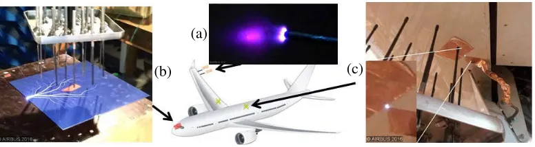
Static charging of an aircraft surface can lead to electromagnetic interference on aircraft radio and avionic systems. These effects were first observed in the beginning of the 20th century, when aircraft began to operate under all weather conditions. The relation between static noise in radios (associated with electrostatic charging) and precipitation conditions led to the name Precipitation Static (P-Static) [1]. Studies following World War II allowed a better understanding of aircraft charge and discharge mechanisms. They showed that an aircraft is charged in-flight mostly by three mechanisms that are triboelectric charging, engine exhaust charging and exogenous charging (cross electric field). However, triboelectric charging is the most considered phenomena as it occurs mainly when an aircraft flies in precipitation conditions (clouds, storms, snow . . . ), and can result in disturbances on communication and navigation systems [2]. The electric charge deposited on the aircraft surface, leads to electrical discharges from the aircraft, which generate the electromagnetic noise responsible for P-Static. These are corona discharges from aircraft extremities [3] surface discharges (streamers) that can take place on insulating surfaces [4], and arc discharges (sparks) that take place in the gap between two metallic parts electrically disconnected (bonding defect) (Figures 1(a), (b) and (c) respectively). These discharges have been well described and studied in the past [5].
Moreover, P-Static has been studied since several decades with for instance test campaigns led at the US Navy [6] or with Boeing commercial airplanes [7], or on helicopter with S-70B-2 Seahawk version of Royal Australian Navy [8]. These studies resulted on the development of techniques to alleviate P-Static, some of which are used nowadays as standards on every aircraft. In fact, current design rules manage the discharge of the aircraft through different solutions that are presented in [9]. They consist of static dischargers (or static wicks) implemented at aircraft structure and that maintain
Received 15 December 2015, Accepted 8 February 2016, Scheduled 18 February 2016
* Corresponding author: Ivan Garcia-Hallo ([email protected]).
1 Airbus Operations, Toulouse, France. 2 Universit´e de Toulouse; INP, UPS; LAPLACE (Laboratoire Plasma et Conversion
(a)
(b) (c)
Figure 1. Electrostatic discharges on the aircraft surface. (a) Corona. (b) Streamer. (c) Arc.
corona discharges at low radiated levels, as well as painting specifications for electric charge flow and bonding specifications to avoid arcing. Some documents provide guidance for design like ARP5672 [10]. In several cases, communications disturbances were reported to be caused by bonding issues, i.e., arcing [1]. The hardest part of the troubleshooting process for P-Static is thus the search for bonding defects, using several known tools (artificial charge application, ohmmeter) [10]. Electric charge can be deposited on the surface of the aircraft by means of low noise corona or pressurized charged air. If sufficient charge is deposited on an unbonded element, an arc discharge takes place in the gap between this part and the rest of the airframe. It can be monitored using a communication device. However, high voltage methods can be hazardous to persons and there is a risk of fuel ignition. Moreover, as the whole aircraft has to be scanned, several days of tedious work are required.
In this article a new solution to this problem is presented, which aims to complement the troubleshooting process of ARP5672 [10]. The proposed tool is composed of several sensors placed on the outer surface of an aircraft, connected to an acquisition system. Then a post processing location method is applied. The proposed system may be able to estimate the position of the static noise source via its electromagnetic emissions. Then, once the aircraft is on ground, only a reduced surface is tested using classical tools, allowing faster troubleshooting process and correlation between a given bonding defect and a given P-Static issue.
2. LOCATION METHOD
A P-Static source generates electromagnetic pulsed emissions that can be picked up by sensors. This way, a collection of pulsed signals is obtained. Then, a post processing phase (location method) takes place in order to extract information from these measurements, that can lead to an estimation of the position of the source. Electrostatic discharge location is a topic that has been largely studied in the past, mostly for partial discharges in high voltage facilities [11–13]. Several methods exist in order to locate a wideband source and in the vast majority of cases it involves the use of an array of sensors. The nature of the sensors can be acoustic, electromagnetic (VHF/UHF), optic and even chemical [14, 15]. In most cases the delay between measured signals is used as an input for a location method and it is also the case for the proposed method.
2.1. Time Delay Estimation
2.2. Hyperbolic Location Method
The delay between signals is used as input for the location method. To illustrate the principle of these methods let’s consider an array of sensors and a transient electromagnetic source. As the sensors are separated by a given distance, the signal coming from the source reaches the sensors at different times, thus allowing an estimation of the Time Of Arrival (TOA) or the TDOA between signals as it will be illustrated later in Section 3.2. Once the TOAs or TDOAs are known, a location can be made either using sphere equations or hyperbolic equations respectively. For example, a 3D arrangement of three sensors (A0,A1, A2) and a partial discharge source that radiates in all directions is presented in Figure 2(a) and on the plane in Figure 2(b).
(a) (b)
Figure 2. (a) Representation of sphere equations for three sensors. (b) Representation of hyperbolic equations for three sensors.
If the TOA to first sensor is known, the delays between signals allow a determination of the distances between the source and each sensor, as described in [17]. The source position is placed at the intersection of spheres, whose radiuses are dependent of the TOA. On the contrary, if the TOA to first sensor is not known, TDOAs can be calculated and sphere equations can be arranged to represent hyperbolic equations as in [17]. The source position is represented by the intersection of these hyperboloids. On a plane, this is represented in Figure 2(b). However, in general, if a source is to be located on a 3D distribution of sensors, four sensors are needed to obtain a unique solution given that there are four unknowns (x, y, z and TOA to first sensor). There would be 4 sphere equations and 3 hyperboloid equations. It is important to note that the number of sensors used has a big impact on the location precision [18]. Moreover, in order to solve these equations to find the source position it is necessary to use numerical methods as Least Squares (LS) [13], Newton-Raphson, [11] or others [19], to reach an approached solution. An exact solution to sphere equations can be found in [20]. These hyperbolic location methods perform very well when all sensors are in LOS with respect to the source. Moreover the precision is improved when the source is placed between all sensors [12]. However, in the context of this paper, the discharge takes place on the surface of an aircraft, a convex structure with sensors placed on the surface. In most positions, sensors and discharge are in NLOS conditions and can be subjected to pulse distortion as in [16], depending on the geometry of the considered path. Given this situation, a localization method that takes into account the geometry of the aircraft is needed.
2.3. TDOA-Based Inverse Method 2.3.1. TDOA-Based Method Principle
Figure 3. Inverse method process.
considerations for signal propagation. Unlike hyperbolic location methods, this allows the use of two sensors minimum to estimate possible source positions as in Section 3.3, as the source is necessarily on the surface of the structure. A simplified computer 3D model of the structure (mock-up, aircraft) is created. The surface of the model is then discretized into a collection of points. Then, each point is considered as a source, one at a time, and the distances to sensors are calculated using a propagation model. The distances to every sensor are then converted to TDOAs and stored, thus creating a database of TDOAs to sensors and the associated source positions. Thus, in the case of an aircraft, when P-Static phenomena occurs in flight, the measured TDOAs to sensors are compared to those of the database and possible source positions are obtained. This process is presented in Figure 3.
The base of the location method is the propagation model as it conditions the TDOAs stored in the database, and therefore the accuracy of the source estimation.
2.3.2. ESD Signal Propagation Model of Mock-up
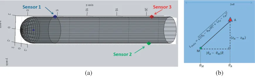
A simplified model is developed for an aircraft fuselage using MATLAB. It consists of a cylinder that represents the fuselage, and a half-sphere for the cockpit. Three sensors are considered on the outer surface (Figure 4(a)) in order to increase location accuracy.
(a) (b)
Figure 4. (a) Simplified fuselage/cockpit model. (b) Helix length equation.
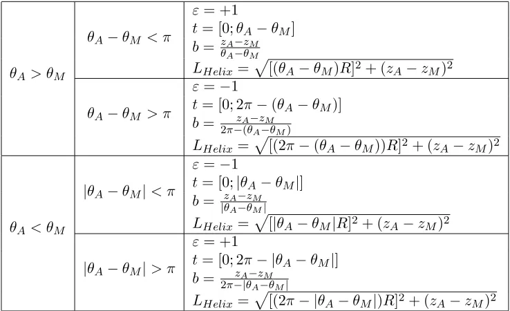
θA> θM
θA−θM < π
ε= +1
t= [0;θA−θM] b= zA−zM
θA−θM
LHelix=[(θA−θM)R]2+ (zA−zM)2
θA−θM > π
ε=−1
t= [0; 2π−(θA−θM)] b= 2π−zA(θ−zM
A−θM)
LHelix=[(2π−(θA−θM))R]2+ (z
A−zM)2
θA< θM
|θA−θM|< π
ε=−1
t= [0;|θA−θM|] b= zA−zM
|θA−θM|
LHelix=[|θA−θM|R]2+ (zA−zM)2
|θA−θM|> π
ε= +1
t= [0; 2π− |θA−θM|] b= zA−zM
2π−|θA−θM|
LHelix=[(2π− |θA−θM|)R]2+ (zA−zM)2
For each point on the cartography of the surface of the cylinder, a helix propagation model is programmed. This model computes the distance between a discretization point and the sensors following the shortest helix possible. The shortest helix is computed following a case-by-case study (Table 1). The surface of the cylinder can be unrolled to become a plane in which the helix becomes a simple line. Using Pythagoras’s relation the calculation becomes simple as in Figure 4(b). In order to test the program, the parametric equations of the shortest helix linking two random points on the surface of a cylinder are used [21]:
H(t) =
x(t) =Rcos(t+εθ
M) y(t) =εRsin(t+εθM) z(t) =zM +bt
(1)
With:
• θA is the angle in cylindrical coordinates for points A, the receiver sensor, and for point M, the
transient source.
• The coordinates of the receiver sensor Aand the transient source M:
A
x
A=Rcos(θA) yA=Rsin(θA)
zA
M
x
M =Rcos(θM) yM =Rsin(θM)
zM
(2)
• b is the reduced lead of the helix. It represents the length of translation for a rotation angle of 1 rad.
• ε= +1 or−1 is a parameter that forces the right (+1) or left (−1) rotation direction of the helix. • ε = +1 or −1 is a parameter that fixes the correction of the length of the helix (ε=ε).
In order to consider the shortest possible helix, four different cases have to be addressed, they are presented in Table 1.
2.3.3.1. Shortest Path on a Sphere
Figure 5. Geometry conventions for great circle calculation.
follows a great circle (a circle that has the same center as the sphere and the same radius) [22]. In spherical and cartesian coordinates, points P and Q on the surface of the sphere can be defined as in Figure 5. The corresponding equations are the following:
PSpherical
R
latp
lonp
PCartesion
x
p =Rcos(lonp) cos(latp)
yp=Rsin(lonp) cos(latp)
zp =Rsin(latp)
(3)
Additionally, letα be the angle between vectors P and Q. It can be determined using definition of the scalar product. The length of the shortest path betweenP andQ is the length of the circle arc, which leads to the following expressions:
α= cos−1
P · Q R2
Circle arc length: P Q =Rα (4)
The TDOA between a source on the cockpit and a sensor can be determined using the length of the circle arc.
2.3.3.2. Shortest Path on Simplified Fuselage
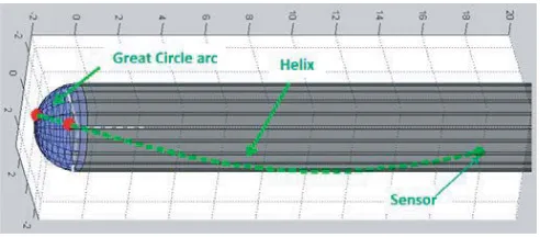
As the shortest path between two points on the surface of a cylinder and a sphere are respectively a helix and a great circle arc, for a combined structure, the shortest path will be a combination of a helix and a great circle arc (Figure 6).
Figure 6. Shortest path on a combined cylinder/half sphere model.
The intersection point between the cylinder and the sphere is found by minimizing the sum of the resulting helix length and circle arc length.
2.3.3.3. Shortest Path on LOS Conditions
(a) (b)
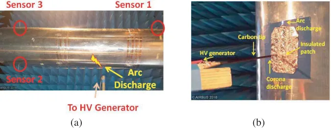
Figure 7. (a) Aircraft fuselage downscaled mock-up. (b) Arc discharge generation setup.
3. EXPERIMENTAL RESULTS ON CYLINDER MOCK-UP 3.1. Measurement Setup
In order to validate the propagation models to be used with the inverse method, a mockup is built. First, a 1 : 6.5 downscaled fuselage mock-up is used, it consists in a simple cylinder with 60 cm diameter. Three identical simple UHF sensors are placed on the surface as they are widely used for these applications [13]. These sensors are actually three identical 7 cm-long whip antennas that operate around 1 GHz. They are connected to three synchronized channels of a digital oscilloscope (Lecroy WR640ZI, bandwidth 1 GHz, Sample rate 20 Gs/sec) using identical cables in order to have the same added delay for each sensor. An arc discharge is generated at the surface of the cylinder using a High Voltage generator (Spellman SL40150) that charges an insulated metallic patch by means of low noise corona (Figure 7). The emissions of this arc discharge are measured using the UHF sensors. As the test setup is placed in an anechoic chamber, reflection paths are avoided, leaving only surface propagation along the cylinder surface.
3.2. Signals Measured at Sensors
The measured signals at the sensors outputs are the following (Figure 8(a)).
In fact, once a collection of signals is obtained by measurement (Figure 8), a characteristic extremum is used as a reference for time delay. For this study, the first minimum is considered. The time reference value is read using a marker leading to an error associated to the marker position. This may be a problem when the first extrema are not trivial to identify. In the case of Figure 9, all signals present a minimum that can be easily identified. An error tolerance of 100 ps is estimated around the marker to
100 ps
(a) (b)
Sensor Output (V)
Sensor Output (V)
Sensor Output (V)
take into account the error on marker placement. For each signal, the time corresponding to the first minimum is notedTi, and the error is included using an interval:
Textrema,i= [Ti,min;Ti,max] =
Ti−error2 ;Ti+error2
(5)
The TDOAs are then calculated using interval arithmetic:
T DOAi,j = [Ti,min;Ti,max]−[Tj,min;Tj,max] = [Ti,min;Tj,max;Ti,max;Tj,min] (6) These TDOA intervals are used for comparison with the TDOA database of the model, and will give more possible sources taking into account the marker positioning error. In the frame of this paper, only the error in determination of the time delay is addressed. However, each source of error is to be taken into account to ensure that the actual P-Static source is included in the estimated zones. In fact, two main sources of error are identified. These are measurement errors and model errors.
They can be described as follows: Error related to measurements
• Dispersion (cables, coupler, sensors, instrumentation).
• Extraction of measurement from ambient signals (phase shift by denoising techniques). • Error in Delay estimation (already taken into account).
Error related to modelization
• Propagation model accuracy and relevancy. • Simplification of the aircraft structure. This process will be addressed in a future work.
3.3. Source Location
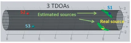
After determination of the TDOA’s (T21, T31, T32) and use of the inverse method described before, a location estimation is obtained for each of the TDOAs represented in a pink area in Figure 8(b), as well as the intersection of these zones represented in a green area in Figure 10.
In Figure 9 the points plotted on the surface of the cylinder are estimated sources obtained by crossing the TDOA database with i) Measured TDOA 2-1 between sensors 2 and 1. ii) Measured TDOA 3-1 between sensors 3 and 1. iii) Measured TDOA 3-2 between sensors 3 and 2. The points from the database that match with the measured TDOAs are plotted in the 3D model. In addition, a tolerance parameter is also used on TDOA values in order to take into account measurement errors (instruments∼100 ps, delay estimation ∼100 ps in the case of this setup). Figure 10 shows the results of the intersection of the three estimated zones i), ii) and iii) of Figure 9.
Figure 9. Estimated sources using one TDOA at a time.
Figure 10. Output for intersection of three TDOAs.
Position Localization accuracy
F1 Within 10 cm radius F2 Within 10 cm radius F3 Within 15 cm radius F4 Within 15 cm radius F5 Within 15 cm radius F6 Within 10 cm radius
Several source positions, presented in Figure 11, are tested and the performances are assessed. The estimated zones contain the real source and, as presented in Table 2, the largest distance around the source is 15 cm (possible points are represented in green on Figure 10). The estimated precision is therefore within a 15 cm radius and this is the case for all tested points (F1 to F6 in Figure 11).
4. CONCLUSION AND FUTURE WORK
This article presented a novel method for P-Static source location to be used with measurements performed in flight. The propagation helix/circle model for a simplified fuselage is implemented and tested using a mock-up cylinder. Measurements performed on the cylinder mock-up show a rather satisfying correlation between the propagation model and measurements as the located sources are at most within a 15 cm radius from the real source. This validates the geometric approach for the estimation of TDOAs for source location.
The next step is to implement propagation models for wings and tail stabilizers and to validate those models using the same approach as presented in this paper. Furthermore, after the model validation, a ray tracing software (ASERIS-HF from Airbus Group Innovations) and a CAD model of an aircraft will be used in order to increase the fidelity between model and real aircraft. Simulations will be validated with aircraft tests on ground and in-flight.
Several important aspects are to be developed as modeling and testing become more representative and complex. The first is instrumentation. In order to measure ESD pulsed signals in a real environment (real communication signals, electromagnetic noise . . . ) it may be necessary to amplify and filter the sensor output before applying the location method.
The second one is to automate post-processing of the measured signals, to determine the time delay between signals as precisely as possible.
The third one is the error management. In fact, the presented measurements attest that the location method principle is valid and the inverse method is able to estimate possible source positions. But in the case of a more complex propagation model and as in the final system, these sources of error are to be taken into account in the inverse method in order to ensure that the estimated zones on the aircraft surface contain the real source.
As a Static troubleshooting tool, this system can complement the troubleshooting process of P-Static events and potentially reduce the duration and number of interventions for bonding fault search.
REFERENCES
1. Nanevicz, J. E., “Static charging effects on avionic systems,” Agard Lecture 110, Atmospheric Electricity, Aircraft Interaction, 1980.
2. Nanevicz, J. E., “Flight-test studies of static electrification on a supersonic aircraft,”Lightning and Static Electricity Conference, Culham, April 1975.
Laboratories, Office of Aerospace Research, United States Air Force, Bedford, Massachusetts, April 1961.
4. Garcia-Hallo, I., D. Lemaire, A. Bigand, and I. Revel, “Study of electromagnetic emissions due to surface discharges,” 2015 International Conference on Lightning and Static Electricity, Toulouse, France, September 2015.
5. Taillet, J., “Basic phenomenology of electrical discharges at atmospheric pressure,” AGARD Lecture Series No. 110, Atmospheric Electricity Aircraft Interactions, June 1980.
6. Whitaker, M., “Results of the recent precipitation static flight test program on the Navy P-3B antisubmarine aircraft,”Proceedings, IAGC on Lightning and Static Electricity, April 1991. 7. King, C. H., “P-Static flight evaluation of a large jet aircraft,” FAA CT 83-25-84, 1983.
8. Devereux, R. W., “Royal Australian Navy S-70B-2 P-Static test results using commercial test equipment,” 15th International Aerospace and Ground Conference on Lightning and Static Electricity, Atlantic City, USA, October 6–8, 1992.
9. Nanevicz, J. E., “Alleviation techniques for effects of static charging on avionics,” Agard Lecture 110, Atmospheric Electricity, Aircraft Interaction, 1980.
10. SAE-Aerospace, “Aircraft precipitation static certification,” SAE ARP5672, Aerospace Recommended Practice, December 2009.
11. Bernier, J., G. Croft, and R. Lowther, “ESD sources pinpointed by analysis of radio wave emissions,” Proceedings — Electrical Overstress/Electrostatic Discharge Symposium, 83–87, Orlando, FL, USA, September 25, 1997.
12. Lin, D. L., L. F. DeChiaro, and J. Min-Chung, “A robust ESD event locator system with event characterization,” Electrical Overstress/Electrostatic Discharge Symposium Proceedings, 88– 98, September 25, 1997.
13. Tang, Z., C. Li, X. Cheng, W. Wang, J. Li, and J. Li, “Partial discharge location in power transformers using wideband RF detection,” IEEE Transactions on Dielectrics and Electrical Insulation, Vol. 13, No. 6, 1193–1199, December 2006.
14. Yaacob, M., M. Alseaedi, J. Rashed, and A. Dakhil, “Review on partial discharge detection techniques related to high voltage power equipment using different sensors,” Photonic Sensors, ISSN: 1674-9251, Vol. 4, No. 4, 325–337, 2014.
15. Soomro, I. A. and M. N. Ramdon, “Study on different techniques of partial discharge (PD) detection in power transformers winding: Simulation between paper and EPOXY resin usingg UHF method,”
International Journal of Conceptions on Electrical and Electronics Engineering, ISSN: 2345-9603, Vol. 2, No. 1, April 2014.
16. Zhou, C. and R. C. Qiu, “Pulse distortion caused by cylinder diffraction and its impact on UWB communications,” IEEE Transactions on Vehicular Technology, Vol. 56, No. 4, 2385–2391, July 2007.
17. Potluri, S., “Hyperbolic position location estimator with TDOAS from four stations,” Master Thesis, Faculty of New Jersey Institute of Technology, Department of Electrical and Computer Engineering, January 2002.
18. Tian, Y. and M. Kawada, “Simulation on locating partial discharge source occurring on distribution line by estimating the DOA of emitted EM waves,”IEE J. Transactions on Electrical and Electronic Engineering, Vol. 7, No. S1, S6–S13, 2012.
19. Mizusawa, G., “Performance of hyperbolic position location techniques for code division multiple access,” Master’s Thesis, Electrical Engineering, Virginia Polytechnic Institute and State University, August 1996.
20. Bucher, R. and D. MISRA, “A synthesizable VHDL model of the exact solution for three-dimensional hyperbolic positioning system,”VLSI Design, Vol. 15, No. 2, 507–520, 2002.
21. Stuart, J., “Calculus: Concepts and contexts,” 2005 Brooks/Cole, Cengage Learning, ISBN-13:978-0-495-55742-5, ISBN-10:0-495-55742-0, 695, 2010.