Properties and Computation of the Inverse of the Gamma function

(1)

Western University Western University

Scholarship@Western

Electronic Thesis and Dissertation Repository

4-23-2018 11:30 AM

Properties and Computation of the Inverse of the Gamma

function

Folitse Komla Amenyou The University of Western Ontario

Supervisor Jeffrey,David

The University of Western Ontario

Graduate Program in Applied Mathematics

A thesis submitted in partial fulfillment of the requirements for the degree in Master of Science © Folitse Komla Amenyou 2018

Follow this and additional works at: https://ir.lib.uwo.ca/etd

Part of the Numerical Analysis and Computation Commons

Recommended Citation Recommended Citation

Amenyou, Folitse Komla, "Properties and Computation of the Inverse of the Gamma function" (2018). Electronic Thesis and Dissertation Repository. 5365.

https://ir.lib.uwo.ca/etd/5365

This Dissertation/Thesis is brought to you for free and open access by Scholarship@Western. It has been accepted for inclusion in Electronic Thesis and Dissertation Repository by an authorized administrator of

(2)

We explore the approximation formulas for the inverse function of Γ. The inverse function

of Γ is a multivalued function and must be computed branch by branch. We compare

three approximations for the principal branch ˇΓ0. Plots and numerical values show that

the choice of the approximation depends on the domain of the arguments, specially for

small arguments. We also investigate some iterative schemes and find that the Inverse

Quadratic Interpolation scheme is better than Newton’s scheme for improving the initial

approximation. We introduce the contours technique for extending a real-valued function

into the complex plane using two examples from the elementary functions: the log and

the arcsin functions. We show that, using the contours technique, the principal branch

ˇ

Γ0(x) has the extension ˇΓ0(z) to the branch cut C\]− ∞,Γ(ψ0)] and the branch ˇΓ−1(x) has the extension ˇΓ−1(z) to the branch cut C\]0,Γ(ψ0)], where ψ0 is the positive zero of Γ0(x).

Keywords: Gamma function, inverse function, branch points, branch cut, extension, contours, Stirling formula, Ramanujan formula, Lambert function

(3)

Acknowledgements

I would to extend my gratitude to my supervisor Prof. David Jeffrey and Prof. Rob

Corless for their support and guidance. I also want to thank Eunice Chan and Leili

Rafiee Sevyeri at ORCA laboratory for their support. Lastly, thanks to everyone in the

Department of Applied Mathematics at Western University.

(4)

List of Figures

1.1 Real-valued plot of Γ.The dot points denote the extrema of Γ . . . 4

1.2 Modulus plot of Γ(z). . . 6

1.3 A phase plot of Γ(z). The colours represent the points that have the same argument . . . 7

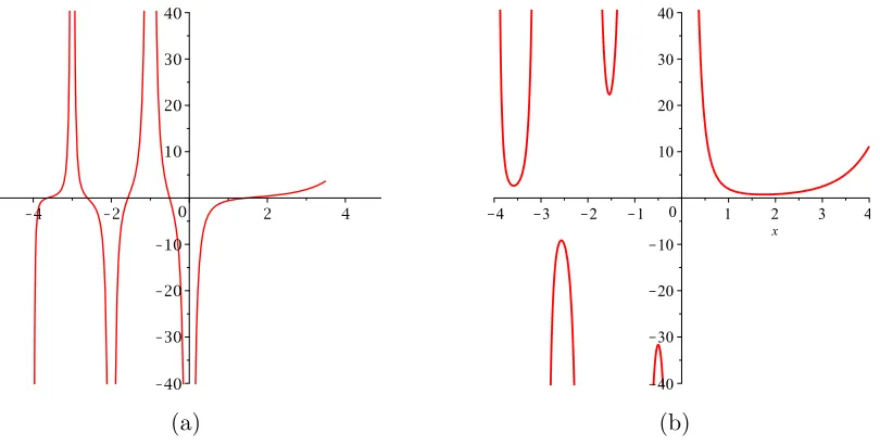
1.4 (a) dΓ/dx. (b) d2_Γ/dx2 _{. . . .} ₇

1.5 (a) dlog Γ/dx. (b) d2_{log Γ/dx}2 _{. . . .} ₈

1.6 Γ(x) and others asymptotic approximations . . . 11

1.7 Γ(x) and other approximations for small values . . . 12

1.8 Γ(x) and other approximations for small values . . . 12

1.9 The condition number Eq. (1.20) of Γ(x) and other approximation for small values. . . 13

1.10 Γ(x) and approximation (1.29). The red dashed lines are the approxima-tion, and the blue dotted lines show Γ(x). . . 15

1.11 A comparison of the Gamma function and Stirling’s formula in the complex plane. . . 16

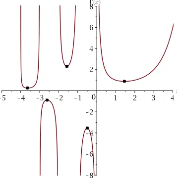
2.1 (a) Real-valued Γ.(b) Real-valued Inverse of Γ. Note the poles in Γ at non-positive integers become the critical points in ˇΓ where the branch changes.The ranges of the branches are shown labelled with k. . . 19

2.2 The principal branch ˇΓ0(red) compared to the ln function(blue). The ln function grows faster than the principal branch. Note that the log function is placed below the principal branch, but will eventually overtake the Inverse Gamma function. . . 20

(8)

2.4 (a) ˇΓ0(x)(red solid) and the approximation (2.12)(blue solid) for larger

argument range.(b) For small argument range. . . 23

2.5 (a) ˇΓ0(x)(red solid ) and the approximation (2.13) (blue) .(b) For small

argument range . . . 24

2.6 (a) ˇΓ0(x)( red solid) the approximation (2.25)(blue solid).(b) For small

argument range. . . 27

2.7 (a) Estimates around the turning point γ0 for approximation (2.26),(b)

Estimates around the turning pointγ0 for approximation (2.31) . . . 31

2.8 Γˇ−1(x)(solid red), the approximation 2.33(blue solid) and 2.34(solid green) 34

2.9 (a) The branch ˇΓ−2(x). The branch ˇΓ−3(x) . . . 35

3.1 Domain and range for complex function mapping in the complex plane . 39

3.2 Extending the log(x) function into the complex plane. The straight

con-tours are trimmed in w-range so that their images do not collide in the

z-domain . . . 40

3.3 Extending the log(x) function into the complex plane. The straight

con-tours are trimmed in w-range so that their images do not collide in

z-domain. Adding the slight slope to the lines makes the collision easier to

see. . . 40

3.4 The range of the Principal value logz in the complex plane. . . 41

3.5 The range of the branchk = 1 of log(z) in the complex plane, denoted ln1z. 42

3.6 Extending the arcsin(x) function into the complex plane. The straight

contours do not need to be trimmed inw-range, and yet the images show

the branch cuts clearly. . . 42

3.7 Extending the arcsin(x) function into the complex plane. The straight

contours above the real axis in the z-domain have been slightly offset

relative to those below the axis, so that the collisions are easily seen. . . 43

3.8 Extending the Principal branch of the inverse of Γ(z) into the complex plane 43

(9)

3.9 Zoom of 3.8(a) . . . 44

3.10 The range of the Principal branch of the Inverse function of Γ(z) in the complex plane . . . 45

3.11 Extending the Principal branch of the inverse of Γ(z) into the complex plane. Contours not starting from the real axis. . . 47

3.12 The range of the principal branch. The dotted line shows an approximation to the boundary. The large dots are points on the boundary showing how it extends for values with negative real part. . . 47

3.13 The extension of the positive ˇΓ−1(x) into the complex plane . . . 48

3.14 The extension of the negative ˇΓ−1(x) into the complex plane . . . 48

3.15 The extension of the positive ˇΓ−1(x) into the complex plane . . . 49

3.16 The range of the branch ˇΓ−1 in the complex plane. . . 50

3.17 A schematic presentation of the ranges of the branches of ˇΓkin the complex plane, fork ≤0. . . 51

(10)

List of Tables

1.1 10 extrema points of Γ . . . 4

2.1 Critical values or turning points for branches of ˇΓk . . . 18

2.2 Branches of ˇΓk and their range . . . 18

2.3 Numerical values of ˇΓ0(x), approximation (2.12) and (2.13) . . . 24

2.4 Error for solving Γ(y)−0.93 for y given an initial y0 . . . 28

2.5 Error for solving of Γ(y)−1 for y given an initial y0 . . . 29

2.6 Newton and Inverse Quadratic Interpolation for solving Γ(y)−0.93 for y 30 2.7 Numerical values of approximation (2.12) and approximation (2.13) . . . 32

2.8 Number of iterations nearx=γ0 for branchk = 0. The starting estimate was based on Eqn (2.31). The columns correspond to Newton’s method (NM) and our quadratic scheme (QS). The iteration was continued until the relative error was less than 10−16 _{. . . .} ₃₃

2.9 Numerical values of the approximation (2.12), (2.34) and (2.35) . . . 34

3.1 Numerical computation of ˇΓ0 for larger arguments . . . 45

(11)

Chapter 1 Fundamental Properties of

the

Γ

function

1.1 Introduction

The Γ function1 is one of the most important special functions in mathematics and has

numerous applications, including combinatorics, statistics, probability theory, quantum

mechanics, and solid-state physics. The Gamma function is defined in different ways in

the literature; there are equivalences between the definitions, and some of the

equiva-lences are trivial to prove, while others need more elaboration. We shall introduce a few

fundamental definitions of the Γ function and refer the reader to the literature for other

definitions and proofs. The first definition of Γ started from the idea of extending the

positive integer factorial n =n(n−1)(n−2). . .2.1 to real numbers. The Γ function is an extension of the factorial function with an argument shifted by 1, to real numbers and

complex numbers.

Γ(z) = (z−1)! = Z ∞

0

tz−1e−tdt , <(z)>0. (1.1)

1_{Some authors write “the Gamma function” and some just refer to it with the Greek letter Γ.}

(12)

The above definition of Γ by an improper integral converges absolutely for<(z)>0 and one can use integration by parts to show the recurrence or functional relation

Γ(z+ 1) =zΓ(z) . (1.2)

Inverting the relation, we have

Γ(z) = Γ(z+ 1)

z . (1.3)

The above equation is important as it’s used to extend the Γ(z) defined in (1.1) to a

meromorphic and more general Γ function for all complex numbers, except the negative

integers. The Γ function is singular at negative integers z = −1,−2, . . . with simple poles and the residues at these points are

Res(Γ,−n) = (−1)

n

n! , n ∈N . (1.4)

Another definition of the Γ function is sometimes called the Weierstrass form and defined

by

1

Γ(z) =ze

γzY

k≥1 (1 + z

k)e −z/k

, z ∈_C\ {−1,−2,−3, . . .} , (1.5)

where γ ≈0.577721. . . is called the Euler-Mascheroni constant.

Another property of the Γ function is the reflection formula

Γ(1−z)Γ(z) = π

sinπz , z /∈Z . (1.6)

The Γ function does not have a closed form and must be approximated. For generations,

many researchers, including mathematicians, physicists, numbers theorists and

statisti-cians, have proposed numerous approximations for the computation of the Γ function.

The rest of this chapter will be devoted to the review of some of the most recent

(13)

1.2. Functional properties of the Γ function 3

of some of the most fundamental functional properties of the function that make it a very

special function. For a full review of the properties of Γ and related functions, see [1].

1.2 Functional properties of the

Γ

function

1.2.1 Notation

Most books and references adopted the convention of writing Γ(x) when referring to

real-valued Γ and Γ(z) when referring to the complex-valued Γ. We will adopt the same

convention in this thesis.

1.2.2 Real-valued of

Γ

function

Figure 1.1 shows the real-valued plot of Γ(x). Poles occur at negative integers. The

dots points are the extrema of Γ. The derivation Γ0(x) can be defined in terms of the

logarithm derivation or digamma or psi function.

Ψ(x) = d

dxln Γ(x). (1.7)

The n-order logarithmic derivation, also called the polygamma function is defined as

Ψ(n, x) = d

n

dxn ln Γ(x) . (1.8)

Table 1.1 shows the 10 extrema of the Γ function and the values Γ at these points. A

few particular values of the Γ function can be computed using the reflection formula

Γ(1 2) =

√ π

by replacing z by 1/2 in the reflection

(14)

Γ(x)

x

Figure 1.1: Real-valued plot of Γ.The dot points denote the extrema of Γ

x Γ(x)

1.46163 0.885603 −0.50408 −3.544644 −1.57349 2.302407 −2.61072 −0.888136 −3.63529 0.245127 −4.65323 −0.052780 −5.66716 0.009324 −6.67841 −0.001397 −7.68778 0.000181 −8.68576 −0.000020

(15)

Γ(−1

2) = −2 √

π

Using the reflection formula Γ(3 2)Γ(−

1 2) = −

√

π and the recurrence relation Γ(z+ 1) =

zΓ(z)

1.2.3 Complex-valued

Γ

The graph of a complex function in one variable produces a surface in 4-dimensional

space and this is difficult to picture in our minds because we can only picture 3-D objects.

The development of mathematical tools and software environments in recent years has

encouraged many visualization techniques, see [25]. But the plot of the modulus, also

called analytical plot, and the portrait phase plot still remain the technique wildly used

for the visualization of complex-valued functions. Figure 1.2 and 1.3 show respectively

the modulus and the phase plot of Γ(z). On figure 1.3, the colours represent the points

that have the same argument.

1.2.4 The

log Γ

function

The monotonicity and the convexity of the Γ and functions related to the Γ has attracted

the attention of many authors and are discussed in many papers, see [9, 2, 4]. And it is

known that the Γ function is convex only for positive real arguments and is logarithmically

convex on the whole R domain. A practical way to verify this is to use the fact that:

• The derivative of a convex functiong of one real variable on the interval [α, β]⊆R is monotonically increasing

• The second-derivative of a convex function g of one real variable on the interval [α, β]⊆R is positive∀x1, x2 ∈[α, β].

For Γ function, the derivative is given by

d

(16)

Figure 1.2: Modulus plot of Γ(z).

and the second derivative is given by

d2

dx2Γ(x) = Ψ(1, x)Γ(x) + Ψ(x)

2_Γ(x) _(1.10)

Figure 1.4 plots the derivative and second derivative of the real-valued Γ. The graph of

dΓ/dx is not that much informative but the graph d2_Γ/dx2 _{clearly shows} _d2_Γ/dx2 _> ₀

∀x∈R+.

For the log-convex property of the Γ function, we use the Weierstrass form

1

Γ(x) =xe

γx

∞ Y

n=1 (1 + x

n)e

(17)

Figure 1.3: A phase plot of Γ(z). The colours represent the points that have the same argument

(a) (b)

(18)

log Γ(x) = −logx−γx+ ∞ X

n=1 x

n −log(1 + x n)

(1.12)

The derivative of log Γ(x) is exactly what is called the digamma function

d

dx(log Γ(x)) = Ψ(x) = Γ0(x)

Γ(x) =−γ+ ∞ X

n=0

1 n+ 1 −

1 x+n

(1.13)

and the second derivative of the log Γ(x) is

d2

dx2(log Γ(x)) = Ψ(1, x) = ∞ X

n=0 1

(x+n)2 (1.14)

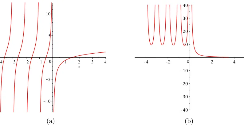
Figure 1.5 (a) shows the plot of the d(log Γ)/dx. It has vertical asymptotes at the points

−n. On each interval (−n,−n+ 1), n ≥1, the function Ψ increases strictly. Figure 1.5

(a) also shows the unique points xn ∈ (−n,−n+ 1), n ≥ 1, such that Ψ(xn) = 0 or

equivalently Γ0(xn) = 0. Also, figure 1.5 (b) shows d2log Γ/dx2 >0,∀x∈R

(a) (b)

(19)

1.3. Numerical approximations of the Γ function 9

1.3 Numerical approximations of the

Γ

function

The numerical computation of the Γ function has attracted the attention of many

re-searchers for generations, all trying to establish the approximation formula that best

computes the Γ function. Many approximation methods have been proposed so far in

the scientific literature. See, [12, 22, 21, 6, 17, 18]. Software libraries and computing

envi-ronments use combinations of these approximations formulas to implement their routines

for Γ. In the following sections, we give a brief overview of the approximations of the Γ

function. Most approximations treat the real-valued Γ.

1.3.1 Stirling formula

The Stirling approximation is, so far, the most well-known and most-cited approximation

for the Γ function and it is defined as

Γ(x+ 1)∼√2πxx e x exp ∞ X m=1 B2m

2m(2m−1)x2m−1 !

=√2πxx e x exp 1 12x − 1 360x3 +

1 1260x5 −

1

1680x7 +. . .

, x→ ∞

(1.15)

where the Bn are the Bernoulli numbers.

Other formulas that are related to the Stirling formula are the Laplace formula, see [24]

Γ(x+ 1)∼√2πx x

e x

1 + 1 12x +

1 288x2 −

139 51840x3 −

571

2488320x4 +. . .

, x→ ∞ (1.16)

and the Ramanujan formula, see [24]

Γ(x+ 1) ∼√2πxx e

x 1 + 1

2x + 1 8x2 +

1 240x3 −

11 1920x4 +

79 26880x5. . .

1/6

(20)

In [17], the author finds an explicit formula for the computation of the coefficients of the

expansion in the series of the expression

exp ∞ X

m=1

B2m

2m(2m−1)x2m−1 !

(1.18)

and gives the following asymptotic approximation

Γ(x+ 1)∼√2πx x

e x

1 + 1 12x2 +

1 1440x3 +

239

36288x6 +. . . x

, x→ ∞ (1.19)

We compare the four approximations mentioned above with the Γ routine implemented in

Maple. Maple guarantees that every built-in function will return numerical values

accu-rate to 0.6ULP2 _{at the current setting of the environmental variable}_Digits_{; ULP means}

Units in the Last Place. In what follows we shall assume that Maple’s approximation

satisfies their promise.

Figure 1.6 shows Maple’s values and the four approximation formulas, where the

number that follows the name of the approximation is the exponent of (1/x) of the last

term kept in the series expansion. As expected, the graphs of the approximations overlap

for larger values of the argument x because they are all asymptotic approximations.

It is almost impossible to see the different colours used to depict the graph of each

approximation.

For small values ofx, the difference between the approximations starts to appear and

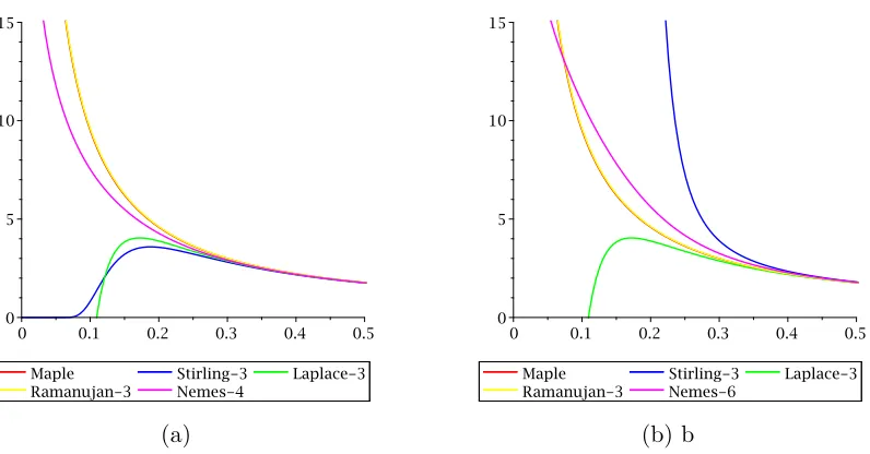
if we zoom the figure 1.6 in the range x∈[0,0.5], we get figure 1.7 and figure 1.8. Figure 1.7 (a) shows that Laplace-1 gives a better approximation than

Ramanujan-1 and Nemes-2, however figure Ramanujan-1.7 (b) and figure Ramanujan-1.8 (a) show that Ramanujan-2 and

Ramanujan-3 outperform the corresponding Laplace-2 and Laplace-3, and Nemes-4. In

all cases, Ramanujan approximation seems to be the approximation that closely agrees

with the Maple Γ built-in function for small values. Another interesting remark is that

the slope of the graph of Nemes and Ramanujan approximations have almost no change

(21)

Γ(x)

x

Figure 1.6: Γ(x) and others asymptotic approximations

as more terms are added in the series expansion. Numerically, it suggests these

approx-imations are more stable than Laplace’s and Stirling’s. We access the stability of the

approximations by computing and plotting their condition numbers. For the evaluation

of a functiony =f(x), the condition number is given in [5]

C(x) = xf 0_(x)

f(x) (1.20)

Figure 1.9 plots the condition number of the five approximations and we can see that

Maple, Ramanujan and Nemes approximations are well conditioned for small values of

(22)

(a) (b)

Figure 1.7: Γ(x) and other approximations for small values

(a) (b) b

Figure 1.8: Γ(x) and other approximations for small values

Ramanujan approximation is shadowed by the red colour of the Maple approximations

suggesting that the Maple routine is based on the Ramanujan approximation. The

Stir-ling and Laplace approximations are poorly conditioned for small values of x and their

(23)

C(x)

x

Figure 1.9: The condition number Eq. (1.20) of Γ(x) and other approximation for small values.

1.3.2 Lanczos approximation

Another well-known and well-cited approximation of the Γ function is the Lanczos

ap-proximation introduced in 1964 in the paper [12] defined as

Γ(x+ 1)≈√2π(z+r+ 1 2)

z+1/2_e−(z+r+1/2)_S

r(z) (1.21)

where

Sr(z) =

1

2a0(r) +a1(r) z

z+ 1 +a2(r)

z(z−1)

(z+ 1)(z+ 2) +. . . (1.22)

(24)

1.3.3 Spouge approximation

Another approximation of the Γ function is the Spouge formula [22]. It is defined by

Γ(x+ 1) ≈√2πe−(z+a)(z+ 1)z+1/2 c0+

N

X

k=0 Ck

z+k +(z) !

(1.23)

where <(z+a)>0 and a∈R,N =dae −1, and ck(a) is defined by the recurrence

c0(a) = 1

ck(a) =

1 √

2π

(−1)k−1

(k−1)!(−k+a)

k−1/2_e−k+a

(1.24)

1.3.4 Other approximations of

Γ

There are many approximations of the Γ function. A comprehensive list of these

ap-proximations can be found in [14]. Most of the apap-proximations are asymptotic, meaning

they accurately compute Γ function for large values of x in the real case and |z| in the complex case. Also, most of the approximations have the similar algebraic form and can

be described by more general formulas. This is the work of [16, 15] who introduced a

couple of family of approximations.

Γ(x+ 1) ∼√2πe.e−a

x+a e

x+1₂

, x→ ∞ (1.25)

where a ∈ R and a ∈ [0,1]. Recently, [24] proposed two general approximations and showed that other approximations are just special cases of his proposed approximation.

Γ(x+ 1)∼√2πx x

e x 1

ea

1 + b

x

cx+d ∞ X

n=0 αn

(x+h)n

!xl_r+q

, x→ ∞ (1.26)

Γ(x+ 1)∼√2πx x

e x 1

ea

1 + b

x cx+d

exp ∞ X

n=0 ψn

(x+h)n

!

, x→ ∞ (1.27)

(25)

1.4. Approximations for negative arguments 15

1.4 Approximations for negative arguments

Stirling’s formula and related approximations apply to positive real arguments.

Approxi-mations for negative arguments are not usually considered, but can be constructed easily.

We rewrite the reflection formula (1.6) using x=−X, so that X >0, as

Γ(x) = Γ(−X) = π

sin(−πX)Γ(1 +X) . (1.28)

We now approximate Γ(1 +X) using Stirling’s approximation (1.15) and obtain

Γ(x)≈ π

sin(−πX)√2πXXX_e−X =

r π 2

e X

X −1

√

Xsin(πX) . (1.29)

Plots of Γ(x) and its approximation are shown in figure 1.10.

(26)

1.5 Approximations for complex arguments

The many publications concerning Stirling’s and similar formulas discuss only real

pos-itive arguments of the function. We have checked its validity in the complex plane as

well. We compare the real and imaginary parts of Γ(z) and Stirling’s approximation on a

contour parallel to the imaginary axis. Figure 1.11 plots Γ(2 +iy) and the corresponding

Stirling’s formula for|y| ≤10. Even so close to the imaginary axis, the approximation is very good. Further from the imaginary axis, the approximation is even better.

(a) Comparison of real parts. (b) Comparison of imaginary parts.

Figure 1.11: A comparison of the Gamma function and Stirling’s formula in the complex plane.

1.6 Conclusion

In this chapter, we reviewed some of the fundamental properties of the Gamma function.

We also covered some approximations of the Γ function. An important challenge that

must be addressed, while suggesting an approximation formula for the Γ function is that

the approximation method must be optimized for small values of the argument. In the

next chapter, we shall use some of the approximation of the Γ for the computation of the

(27)

Chapter 2 Real Inverse function of

Γ

2.1 Introduction

The Inverse function of Γ has applications in computer science [8]. It is a multivalued

function. In a recent review of Γ in [1] the authors have pointed out that the Inverse

function of Γ has received less attention. Some of the basic properties of the Inverse

function of Γ were studied in [19]. In the papers [23] and [19], the authors showed that

the Principal branch or the Principal Inverse of the Inverse function of Γ has an extension

to a Pick function1 in the cut plane _C\]− ∞,Γ(ψ0)], whereψ0 ≈1.4616. . . . But there is no study of the numerical and symbolic computation of the Inverse function of Γ.

In this chapter and the next, we intend to explore some numerical procedures for the

computation of the branches of the Inverse function of Γ.

2.2 Notation and branches definition

We denote the Inverse function of Γ(x) by w = ˇΓk(x), where k labels the branch. The

extrema of the Γ function defined by

d

dxΓ(x) = Γ(x)Ψ(x) = 0 (2.1)

1_{See reference [19] for the definition of Pick functions}

(28)

and we denote these points (ψi, γi)       

Ψ(ψ0) = 0 where ψ0 >0

Ψ(ψk) = 0 where k <0 and k < ψk < k+ 1

Numerical values of these points are displayed in table 2.1. The branches ˇΓk are defined

k ψk γk = Γ(ψ0) 0 1.461632 0.885603 −1 −0.504083 −3.544644 −2 −1.573498 2.302407 −3 −2.610720 −0.888136 −4 −3.635293 0.245127 −5 −4.653237 −0.052780

Table 2.1: Critical values or turning points for branches of ˇΓk

by the interval or the domain of the arguments and the range of ˇΓk is displayed in table

2.2. Using the notation x = Γ(y), and y = ˇΓk(x), if x falls outside the intervals shown

above, ˇΓ becomes complex-valued. The numbering is chosen so that k = 0 corresponds

k Arguments Intervals Range of ˇΓk

0 x≥γ0 ψ0 ≤Γˇ0

−1 x > γ0 0<Γˇ−1 < ψ0 x≤γ−1 ψ−1 ≤Γˇ−1 <0

−2 x < γ−1 −1<Γˇ−2 < ψ−1 x > γ−2 ψ−2 ≤Γˇ−2 <−1

Table 2.2: Branches of ˇΓk and their range

to the principal branch or principal Inverse and the remaining branches receive negative

numbers so that the labels follow roughly the range taken by the branches. We notice

some special values, since Γ(2) = 1! = Γ(1) = 0! = 1, the corresponding Inverse must

lie on different branches. This requires ˇΓ0(1) = 2 and ˇΓ−1(1) = 1. Some other special

values of interest are ˇΓ0(

√

(29)

2.3. Visualization of the Inverse function of Γ 19

ˇ Γ−1(

√

π) = 1/2. In this chapter, we will denote the approximations of the Inverse

function of Γ by y(x), where x is the real argument.

2.3 Visualization of the Inverse function of

Γ

We can plot the real-valued Inverse function of Γ using the known procedure for Γ. Recall

that the plot command in Maple for x= Γ(y), given an input y, is

plot([y,GAMMA(y),y = a..b],discont=true,view =[a..b,c..d])

The plot of the Inverse function of Γ(y) is obtained by exchanging x and y, that is

y= ˇΓk(x) and the Maple command becomes

plot([GAMMA(x),x,x=c..d],discont=true,view = [a..b,c..d])

(a) (b)

Figure 2.1: (a) Real-valued Γ.(b) Real-valued Inverse of Γ. Note the poles in Γ at non-positive integers become the critical points in ˇΓ where the branch changes.The ranges of the branches are shown labelled withk.

Figure 2.2 compares the principal branch to the ln function. The Inverse Gamma

(30)

Figure 2.2: The principal branch ˇΓ0(red) compared to the ln function(blue). The ln function grows faster than the principal branch. Note that the log function is placed below the principal branch, but will eventually overtake the Inverse Gamma function.

2.4 The condition number of the Inverse function

The condition number is a well-known parameter used to compare the stability of the

evaluation of a function. In this section we show a method to plot the condition number

of the Inverse of a function only using the function itself. Given any function g(x), and

a pointx,the condition number C at x is defined [5] by

C(g, x) = xg 0_(x)

(31)

2.4. The condition number of the Inverse function 21

Assume we know a function f and we want to plot, or calculate, the condition number

for evaluating its inverse ˇf. We write the function and its inverse as a pair of equations:

y = ˇf(x), (2.3)

x=f(y) . (2.4)

In our case, we want C(ˇΓ, x). We begin by recalling an elementary result. Differentiate

the above equations w.r.t. x.

dy dx =

df(x)ˇ

dx (2.5)

1 =df dy

dy

dx (2.6)

From the pair above and equation

ˇ

f0(x) = d ˇ f(x)

dx = 1

df(y)/dy (2.7)

Therefore we have a parametric representation for the condition number:

C( ˇf , x) =xfˇ 0_(x)

ˇ f(x) =

x

(df /dy) ˇf(x) (2.8)

= f(y)

(df /dy)y = 1/C(f, y) (2.9)

From this we see we can treat y as a parameter, and specify the condition number using

y as a parameter. Specializing this to the Γ function, we have

C(ˇΓ, x) =1/C(Γ, y) = 1

yΨ(y) , (2.10)

x=Γ(y). (2.11)

(32)

plot([x(t),y(t),t=a..b])

So in the present case we have

plot([GAMMA(y),1/(y*Psi(y)),y=0.1..1.45])

Figure 2.3 shows the condition number for branch ˇΓ0. It is clear on the figure that the

Inverse function is well conditioned except near the branch points.

C(x)

x

Figure 2.3: The condition number of the inverse function of Γ. Eq. (2.10)

2.5 Estimates for the principal branch

Γ

ˇ

0

In this section, we explore and compare different approximation formulas for the principal

(33)

2.5. Estimates for the principal branch Γˇ0 23

function that is inverted to obtain the Inverse function of Γ. Following the branch

numbering system we adopted earlier, the Principal branch ˇΓ0 of the Inverse function

of Γ is defined for the real arguments in the interval x > γ0 and the corresponding real

range is [ψ0,∞].

2.5.1 Stirling-based approximation

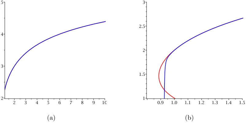
One of the first asymptotic approximation for the computation of ˇΓ0 is proposed in [1]

and is based on the inversion of the original Stirling formula. It is defined by

y(x)∼ 1 2 +

ln(x/√2π) W0(e−1ln(x/

√

2π)) (2.12)

This expression becomes complex for x < e−1√_2π _≈ _{0.92, but delivers a good starting} approximation for x > 1 as we can see on figure 2.4. For x < 1, the approximation

becomes poor and get worse as the argument gets closer to the turning point.

Another asymptotic approximation derived from the Stirling formula and suggested in

(a) (b)

(34)

[1] is

y(x)∼ 1 2 +

1 24u0(1 +w)

−(5 + 10(1 +w) + 14(1 +w)

2₎

5760(1 +w)3_u3 0

+. . . (2.13)

where u0 = ln(x

√

2π)/w with w= W0(ln(x/

√

2π)/e). Here again, the expression (2.13)

(a) (b)

Figure 2.5: (a) ˇΓ0(x)(red solid ) and the approximation (2.13) (blue) .(b) For small argument range

delivers a good starting approximation for x > 1 as we can see on figure 2.5. Table

2.3 compares the approximation (2.13) and (2.12) for a few known arguments with the

corresponding relative error ˇΓ0−y

ˇ

Γ0 . The error decreases for both approximations as the

arguments becomes larger, but the error for (2.13) is much smaller than the that of

the approximation (2.12) until value x < 1. It’s around the turning point γ0 that the

expression (2.12) is better than the expression (2.13).

x Γˇ0 Eq. (2.12)/error Eq. (2.13)/error √

π

2 = 0.88623. 3/2 complex complex

Γ(1.8) = 0.93138 1.8 1.64452./8.6% 1.60325./10.8% Γ(1.92321) = 0.96992 1.92321 1.83429./3.6% 1.91500/0.4%

1 2 1.92884./3.6% 1.99700./0.2%

3√π

4 = 1.32934. 5/2 2.47003/1.2% 2.49989./ 4.2×10 −5_%

15√π

8 = 3.32335. 7/2 3.48741./0.4% 3.49999./1.5×10 −6_%

24 5 4.99386./0.1% 4.99999./0%

(35)

2.5. Estimates for the principal branch Γˇ0 25

2.5.2 Ramanujan-based approximation

In this section, we intend to derive a closed form estimate for the principal branch of the

Inverse function of Γ by inverting the Ramanujan formula, [24]. The Ramanujan formula

is defined by

Γ(y)∼ r 2π y y e !y

1 + 1 2y +

1 8y2 +

1 240y3 −

11 1920y4 +

79 26880y5 . . .

1/6

, x→ ∞

(2.14)

inverting the above formula is not simple; we follow the method used in [1]. Applying ln

function to the above equation gives:

ln Γ(y)∼ylny−y+ ln√2π−1 2lny+

1

6lnK (2.15)

where K = 1 + ₂1_y + ₈1_y2 +

1

240y3 . . . The series expansion of lnK in Maple using the

command Series(ln K,x,2), is

lnK ∼ −ln(240) + ln(1/y3) (2.16)

The above equation becomes

ln Γ(y)∼ylny−y+ ln√2π−lny−ln 240/6 (2.17)

We want to solve

x= Γ(y) (2.18)

for y when x becomes large. Posing v = x/√2π, and K1 = −ln 240/6, the equation (2.18) becomes

(36)

Dropping the term lny, the equation (2.19) becomes

ylny−y= lnv−K1 (2.20)

y e ln

y e =

1

e(lnv−K1) (2.21)

(lny e)e

lny/e ₌ 1

e(lnv−K1) (2.22)

Using the Lambert Wfunction,

lny e =W

1

e(lnv−K1)

(2.23)

and

y e =e

W

1

e(lnv−K1)

= 1

e(lnv−K1)

W1

e(lnv−K1)

(2.24)

given

y= ln(x/

√

2π)−K1 W1_e(ln(x/√2π)−K1)

(2.25)

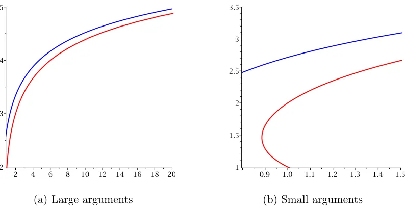
Figure 2.6 shows that the expression (2.25) is far from delivering a good starting value

for the principal branch ˇΓ0 even asymptotically as it was the case for the two previous

approximations. But at least, the graph of the approximation (2.25) seemed to have the

same slope as the graph of ˇΓ0, suggesting that any simple iterative scheme might help to

improve the solution.

2.6 Iterative Schemes

The three approximations formulae we investigated so far are obtained by inverting a

particular Γ approximation, by solving the equation Γ(y) = x for y. This suggests that

an iterative scheme can be used to improve the solution given an initial estimate. In this

section we test a few, well-known iterative schemes and compare the solution for small

(37)

2.6. Iterative Schemes 27

(a) Large arguments (b) Small arguments

Figure 2.6: (a) ˇΓ0(x)( red solid) the approximation (2.25)(blue solid).(b) For small argu-ment range.

iterative schemes are:

• Cost of initial estimate. More time spent on obtaining a better estimate can reduce

the number of iterations.

• Cost of an iteration. This is affected by the choice of the function used for the iteration, and the order. Maple has implemented both a GAMMA function and a

lnGAMMAfunction. Either could be used for the iteration.

• The order of the iteration scheme. By using a higher-order scheme, one can reduce

the number of iterations.

2.6.1 Newton Schemes

To solve Γ(y)−x= 0 for y, given an initial approximation y, the Newton procedure in Maple is

Newton:= proc(y,x) local Gtmp,f,fprime;

Gtmp:= G(y);

(38)

fprime := Psi(y)*Gtmp;

return y-f/fprime;

end proc:

Below, we rewrite the three closed form formula for the Principal branch ˇΓ0

y(x)∼ 1 2 +

ln(x/√2π) W0(e−1ln(x/

√

2π)) (2.26)

y(x)∼ 1 2 +

1 24u0(1 +w)

−(5 + 10(1 +w) + 14(1 +w)

2₎

5760(1 +w)3_u3 0

+. . . (2.27)

where u0 = ln(x

√

2π)/w with w=W0(ln(x/

√

2π)/e).

y(x)∼ ln(x/ √

2π)−K1 W1_e(ln(x/√2π)−K1)

(2.28)

We solve the Γ(y)−x = 0 for two arguments range, for x = 0.93 and x = 1 given an initial estimate from the three above formulas. Table 2.4 and 2.5 shows the backward

error at each iteration. The error decreases for all three approximates of ˇΓ0 but the

k Eq. (2.26) Eq. (2.27) Eq. (2.28) 0 3.2×10−2 _4.2_×₁₀−2 _5.4_×₁₀−1 1 2.1×10−2 _2.1_×₁₀−1 _1.5_×₁₀−1 2 1.7×10−3 4.6×10−2 3.0×10−2 3 1.5×10−5 5.9×10−3 3.1×10−3 4 1.3×10−9 _1.7_×₁₀−4 _4.9_×₁₀−5 5 0 1.7×10−7 _1.4_×₁₀−8

6 0 0 0

Table 2.4: Error for solving Γ(y)−0.93 for y given an initial y0

approximation (2.26) outperform the other two by reducing the error by a factor of

be-tween 10 to 104 within 4 iterations for x= 0.93. But for x= 1, the approximation (2.27)

gives a better approximates of ˇΓ0. In table 2.4, the initial error of the approximation

(39)

k Eq. (2.26) Eq. (2.27) Eq. (2.28) 0 2.8×10−2 1.3×10−3 5.6×10−1 1 2.4×10−3 3.7×10−6 1.4×10−1 2 1.3×10−5 ₀ _2.2_×₁₀−2

3 0 0 9.5×10−4

4 0 0 2.1×10−6

5 0 0 0

Table 2.5: Error for solving of Γ(y)−1 fory given an initialy0

using the relative error (ˇΓ0−y)/Γˇ0as a comparison parameter, that is the approximation (2.27) is better than the approximation (2.26) for all argument except around the turning

point x ∼ e−1√2π where (2.26) does better. In both argument interval, the expression (2.28) demands more iterations. The estimate to choose from depends on the arguments

range. The iterative scheme is effective to reduce the number of iteration only when a

better starting estimate is given.

2.6.2 Inverse Quadratic Interpolation

Inverse Quadratic Interpolation is an iterative scheme like Muller’s scheme, [26],2 that

uses three previous points to extrapolate the next point. But unlike Muller’s method,

Inverse Quadratic Interpolation interpolates the three points with a quadratic inverse

function. To solve Γ(y)−x = 0, for y given three initial estimates y0 , y1 , y2 , the IQI iteration is

IQI:= proc(y0,y1,y2,y3) local x;

f := G(y) - x;

y:= polyinterp([f(y0),f(y1),f(y2)],[y0,y1,y2],0);

y0 := y1;

y1 := y2;

y2 := y;

return y;

(40)

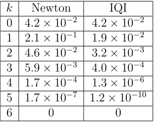
k Newton IQI 0 4.2×10−2 4.2×10−2 1 2.1×10−1 1.9×10−2 2 4.6×10−2 _3.2_×₁₀−3 3 5.9×10−3 _4.0_×₁₀−4 4 1.7×10−4 1.3×10−6 5 1.7×10−7 _1.2_×₁₀−10

6 0 0

Table 2.6: Newton and Inverse Quadratic Interpolation for solving Γ(y)−0.93 for y

end proc:

The problem with IQI is that it requires f(y0),f(y1),f(y2) to be distinct. The only

approximation of ˇΓ0 that can guarantee that is the expression (2.27). The three starting

points will be set as follows

y0 = 1 2 +u0

y1 =y0+

1 24u0(1 +w)

y2 =y1+

(5 + 10(1 +w) + 14(1 +w)2₎ 5760(1 +w)3_u3

0

(2.29)

where u0 = ln(y/

√

2π)/w, with w=W0(ln(y/

√

2π)/e).

Table 2.6 compared the IQI and the Newton’s schemes for solving Γ(y)−0.93 given an initial estimate (2.27). Starting from the same value, ≈ 4.2×10−2_{, the error of IQI} scheme is 10 times smaller than that of Newton’s scheme for the first iterations. And

from the fourth iteration, the error becomes 100 to 1000 times smaller. This shows that

the choice of the iteration scheme can drastically impact the error rate or the number of

iterations before convergence, assuming we have a good initial estimate.

2.6.3 Improving the estimates for small arguments

We saw earlier that all the approximations deliver good starting values forx >1 but do

(41)

use a Taylor series around the turning point x = γ0. For γ0 ≤ x ≤ 1 the Taylor series around γ0 is

Γ(y) =γ0+ 1

2γ0Ψ(1, ψ0)(y−ψ0)

2₊_O((y₋_ψ

0)3) , (2.30)

where the linear term is absent because we expand around a stationary point. Given a

specific value x of Γ(y) =x for which we need the inverse, we solve the equation (2.30)

for y by dropping the error term and solving the quadratic equation:

y∼Γˇ0(x) =ψ0+ s

2(x−γ0) Ψ(1, ψ0)γ0

. (2.31)

The principal branch is given by the positive square root. As we can see on figure

2.7, there more agreement between the approximation (2.31) and ˇΓ0 than (2.26) and ˇΓ0.

Numerical values in table 2.7 shows that around the turning pointγ0, the Taylor equation

gives a better starting approximation than both the expression 2.26 and 2.27.

(a) (b)

(42)

x Γˇ0 Eq. (2.26)/error Eq. (2.27)/error Eq. (2.31) /error √

π

2 ≈0.886 3/2 complex complex 1.5003/0.02%

Γ(1.8)≈0.9314 1.8 1.6445/8.6% 1.603/10.8% 1.788/0.63% Γ(1.92321)≈0.9699 1.923 1.8343/3.6% 1.915/0.4% 1.9052/0.94%

1 2 1.9288/3.6% 1.9970/0.2% 1.9783/1.1%

3√π

4 ≈1.3293 5/2 2.4700/1.2% 2.4999/ 4.2×10

−5_% _2.4793/0.83%

15√π

8 ≈3.3234 7/2 3.4874/0.4% 3.4999/1.5×10

−6_% _3.8468/10%

24 5 4.9939/0.1% 4.9999/0% 8.8063/76%

Table 2.7: Numerical values of approximation (2.12) and approximation (2.13)

2.6.4 The rate of convergence near the turning point

γ

0

It is well known that near a stationary point, Newton’s method degrades from quadratic

convergence to linear convergence. Consequently, near x = γ0, we explore a quadratic

scheme 3_{. We expand around an initial estimate:}

Γ(a) + Ψ(a)Γ(a)(x−a) + 1/2Γ(a)(Ψ0(a) + Ψ(a)2)(x−a)2+O((x−a)3) (2.32)

where Ψ0 is the derivative of the Ψ function. Solving for x gives the iterative scheme

below. To solve Γ(y)−x= 0, given an initial estimate y, the Maple iteration is

QS := proc (y, x) local dx, a, b, c;

a := (1/2)*(Psi(1, y) + Psi(y)^2*G(y);

b := Psi(y)*G(y);

c := G(y)-x;

dx := (1/2)*(-b + sqrt(b^2 - 4*a*c))/a;

return y + dy;

end proc:

Table 2.8 shows the number of iterations needed by Newton’s method and the quadratic

scheme near the stationary point x =γ0. There is a gain of, at most, two iterations for

3_{Note that we are not using a similar scheme called Muller’s method, nor the Inverse Quadratic}

(43)

2.7. Estimates for the branch Γˇ−1 33

x N M QS

1.000 4 2

0.950 3 2

0.900 3 2

0.890 3 2

0.886 3 1

Table 2.8: Number of iterations near x = γ0 for branch k = 0. The starting estimate was based on Eqn (2.31). The columns correspond to Newton’s method (NM) and our quadratic scheme (QS). The iteration was continued until the relative error was less than 10−16

the quadratic scheme over the Newton scheme, but this comes with a drawback in that

one must explicitly evaluate the second derivative of Γ(y)−x and extract a square root.

2.7 Estimates for the branch

Γ

ˇ

₋₁

The branchk =−1 or ˇΓ−1(x) has two real domains and two associated ranges: The pos-itive real domain [γ0,∞] and its positive range [0, ψ0]; and the negative domain ]∞, γ−1] has its negative range ]ψ−1,0[ The first approximation for positive domain of this branch

is proposed in [1] who uses the second branch of the Lambert W function

y(x)∼ 1 2+

ln x/√2π W−1(e−1ln(x/

√

2π)) (2.33)

Another approximation is proposed in [7]

y(x)∼ 1

x (2.34)

Figure 2.8 shows the branch ˇΓ−1(x) and the two approximation. The estimate (2.12)

seemed to be a better starting point for the branch for small arguments range than the

estimate (2.34), but it’s only defined for x ∈ [ √

2π

e ,

√

2π]. The approximation (2.34),

on the other hand is defined on the whole real line. It agrees with the branch as the

(44)

Figure 2.8: ˇΓ−1(x)(solid red), the approximation 2.33(blue solid) and 2.34(solid green)

in the intervalγ0 ≤x≤1 to have a better starting estimate. The Taylor series is defined by

y= ˇΓ−1(x) =ψ0− s

2(x−γ0) Ψ(1, ψ0)γ0

(2.35)

Table 2.9 shows some particular numerical values of the expression (2.12), (2.34) and

(2.35).

x Γˇ−1 Eq. (2.33)/error Eq.(2.34)/error Eq.(2.35)/error

γ0 ψ0 complex 1.1292 /22% 1.4616 / 0%

1 1 1.1254 /11% 1 / 0% 0.945/5.5%

Γ(0.8) = 1.1642_√ 0.8 0.900/ 12.5% 0.8589 / 7.4% 0.6552 / 18%

π 1/2 0.6072 / 21% 0.5641 /12% 0.0229/96%

(45)

2.8. Estimates for other branches Γˇk 35

2.8 Estimates for other branches

Γ

ˇ

k

The other branches of ˇΓk can be obtained with the same procedure.

• Expand Γ(y) around the singular point.

• Keep only one term of the expansion.

• Invert the expansion, by solving Γ(y) −x = 0 for y. The result is the initial approximation of the branch

• Use an iterative scheme to improve the solution

Figure 2.9 shows the approximation of the branch ˇΓ−2and ˇΓ−3 The question is how many

(a) (b)

Figure 2.9: (a) The branch ˇΓ−2(x). The branch ˇΓ−3(x)

branches can we really compute? Not many. As we seek to compute more branches, the

turning points γk = Γ(ψk) become smaller and the and as a consequence ˇΓk(x) → the

pole of Γ(x)

2.9 Conclusion

In this chapter, we explored three different approximations for the numerical

(46)

deliver good starting points for the branches ˇΓk(x) for large argument range but

underper-formed for small arguments. We also show that, once we have a good starting estimate,

an iterative scheme can be used to improve the solution and we compared two iterative

schemes for that matter. Finally, we showed that the estimate to choose from depends

on the arguments range. In the next chapter, we will focus on the extension of ˇΓk(z) in

(47)

Chapter 3 Complex Inverse function of

Γ

3.1 Introduction

The idea of extending the Inverse function of Γ(x) in the complex plane was first

in-troduced by M. Uchiyama in his paper, [23]. He the proved that the principal inverse

of Γ restricted to the interval [α,∞] denoted as Γ−1_{(x) has the holomorphic extension} Γ−1_{(z) to the cut plane}

C\]− ∞,Γ(α)], where α is the unique zero of the logarithmic

derivative Ψ of Γ(x) on the positive half real line. Moreover, [23] showed the extension

Γ−1_{(z) is a Pick function. In [19], the authors got the same result as [23] but on the}

decreased interval [0, α]. Both [23] and [19] based their proof on the L¨owner theorem

that relates the positive semi-definite L¨owner kernel to a Pick function. In the last

Chap-ter, we reviewed some properties of the Inverse function of Γ(x) in the real domain. In

this chapter, we shall extend the Inverse function Γ(x) in the complex plane using the

technique introduced by David J. Jeffrey in [11].

3.2 Notation

Throughout this chapter, the Inverse function of Γ(x) will be denoted by ˇΓk(x) in real

domain and by ˇΓk(z) in the the complex plane, where k denotes the branch number.

(48)

3.3 The extension of

Γ

ˇ

k

(

x

)

to the complex plane

We shall extend the ˇΓk(x) function in the complex plane using the technique in [11].

We describe the general technique first. Let us say we want to extend the real-valued

function y = f(x) in the complex plane. The technique in [11] can be summarized as

follows.

• Denote the desired extension by w=f(z).

• Plot side by side, the realz-domain and the real w-range of f.

• Starting from the real line in thew-range of f, draw a series of lines parallel to the

imaginary axis.

• Map these parallel lines into the z-domain of f using the map w 7→ g(w), where

g(w) is the inverse function off(z).

• Trim the parallel lines in w-range so that their images do not collide in z-domain,

but at the same time fill thez-domain.

• The line along which the images collide in the z-domain is a candidate for the

branch cut.

• Note the range of f(z) in the complex plane. Figure 3.1 shows the z-domain and the w-range of the mapping in the complex plane.

In the next section, we shall prepare the use of the technique in [11] with the examples

of the log(x) function and the arcsin(x) function.

3.3.1 The extension of the log function in the complex plane

It’s well-known that the logz function is a multivalued function and its inverse is the

(49)

3.3. The extension of Γˇk(x) to the complex plane 39

w=f(z) →

←

z =g(w)

(a) z-domain (b) w-range

Figure 3.1: Domain and range for complex function mapping in the complex plane

The logz function is defined as

log(z) = log|z|+iarg(z) z 6= 0

= log|z|+iArg(z) + 2πim, m= 0,±1,±2, . . . , −π <Arg(z)≤π (3.1)

The value of logz are complex numbers w, such thatz = exp(w).

The principal value is defined as

Log(z) = log|z|+iArg(z) , −π <Arg(z)< π . (3.2)

To extend log(x) to the complex plane with the technique described in [11], starting from

the real line, we extend the range ]−∞,∞[ of log(x) into the complex domain by drawing a series of the straight contours parallel to the imaginary axis. The straight contours are

mapped back to the z-domain using the map w 7→ ew_{. The image of the straight lines}

collide along the negative real axis in the z-domain. The intersection is not visible on

figure 3.2 because the principal value and the other branches of the log(z) function have

the same algebraic form, they only differ by±2π.

Although [11] uses lines parallel to the imaginary axis, this is not necessary. If we

(50)

Figure 3.2: Extending the log(x) function into the complex plane. The straight contours are trimmed in w-range so that their images do not collide in the z-domain

3.3, where the collisions can be seen because the contours (now spirals) are passing

themselves. To obtain the principal value of log(z), we must trim them on the imaginary

(a) z-domain _{(b) w-range}

Figure 3.3: Extending the log(x) function into the complex plane. The straight contours are trimmed in w-range so that their images do not collide in z-domain. Adding the slight slope to the lines makes the collision easier to see.

(51)

Figure 3.4: The range of the Principal value logz in the complex plane.

denoted [10] by lnkz, wherek is the branch number. In algebraic terms, the definition is

lnk(z) = Log(z) + 2πik . (3.3)

In graphical terms, the procedure now is to remove from thewplane the region assigned

to the principal branch, and repeat the construction of the two sets of contours in the

remaining space. Figure 3.5 shows the range of ln1z, where the contours have been

trimmed to the region defined byπ < <(z)≤3π.

3.3.2 The extension of the arcsin function in the complex plane

In this section we show another aspect of using contours to visualize branches. The inverse

sine function is periodic in the real direction, different from the logarithm function which

is periodic in the imaginary direction. If we use straight lines parallel to the imaginary

axis, we do not get collisions. The sine function has a period of 2π, but an antiperiod1

[13] of π radians. Therefore we start with the real interval in the w-range [−π/2, π/2]. We obtain the plots in figure 3.6. The branch cuts are clearly |x| ≥ 1. The definition

(52)

(a) z-domain (b) w-domain

Figure 3.5: The range of the branchk = 1 of log(z) in the complex plane, denoted ln1z.

of the branch cuts can also be seen using colliding contours, as was done for logarithm.

This is shown in figure 3.7, where contours parallel to the real axis are used.

(53)

Figure 3.7: Extending the arcsin(x) function into the complex plane. The straight con-tours above the real axis in thez-domain have been slightly offset relative to those below the axis, so that the collisions are easily seen.

3.3.3 The extension of the

Γ

ˇ

0

in the complex plane

The real domain of the principal branch ˇΓ0 is the interval [γ0,∞] and the range [ψ0,∞], where γ0 = Γ(ψ0) and ψ0 is the positive zero of Γ0(x). Following the same process and

using the map w 7→ Γ(w), we get figure 3.8 that shows the images colliding on the negative real line in the interval [−∞,Γ(ψ0)]. Figure 3.9 is a zoom of figure 3.8(a) so

(54)

Figure 3.9: Zoom of 3.8(a)

that we can clearly see the intersection in the z-domain. Continuing with the process,

the straight contours must be trimmed in the w-domain. The question is at what point

w to trim in w-range. This is purely done, at this level, by a simple experimentation.

The contours are trimmed at some random imaginary points and then mapped into the

z-domain. If the image crosses the line of discontinuity, the line are shorten further in the

w-range. This is not an automatic way of doing things but it does help in appreciating

the range of the branches. Figure 3.10 shows the range of the principal branch ˇΓ0 in the

complex plane. The interval [−∞, γ0] = [−∞,Γ(ψ0)] is the branch cut. Figure 3.10 also shows that as the argument z becomes larger, the parallel lines become shorter. That’s

ˇ

Γ0(z)→ <(ˇΓ0(z)) asz becomes large. For complex numbers,z larger means the modulus ofz is larger. This give three possible scenarios, the first is <(z) is a big real number and <(z) =(z), the second is both the <(z) and =(z) are big real numbers of the same

(55)

(a) z-domain (b) w-domain

Figure 3.10: The range of the Principal branch of the Inverse function of Γ(z) in the complex plane

z Γˇ0(z)

1045000_{+ 10}45_i _{2309.20162 + 0.i} 10450000_{+ 10}450_i _{98685.55560 + 0.i} 1045000+ 1045000i 12309.23842 + 0.08339.i 10450000+ 10450000i 98685.58564 + 0.06829.i 1045_{+ 10}45000_i _{12309.20162 + 0.16678.i} 10450_{+ 10}450000_i _{98685.55560 + 0.13659.i}

Table 3.1: Numerical computation of ˇΓ0 for larger arguments

And as we can see in the table 3.1, the contribution of the imaginary part of ˇΓ0(z)

becomes negligible for larger arguments z and ˇΓ0(z)→ <(w).

When the contours shown in figure 3.8(b) are mapped using Γ into 3.8(a), they do

not cover all points in the z-plane. It is necessary for the range to be in one-to-one

correspondence with all of the domain, or else there will be values of z that have no

ˇ

Γ0(z) . Therefore, we need to search for contours that fill in the drop-shaped region

surrounding the origin in the z-plane, which is not yet filled. The required contours

cannot start from the real axis, because the unused portion of the real axis has been

assigned to other branches. This is a new feature of this function, relative to the log and

(56)

In constructing the contours shown in figure 3.11, we have to trim at both the lower

end, which determines the right hand end of the drop shape, and the upper end which

determines the left end. As we have seen, the values of ˇΓ0 tend to zero exponentially for

largez, and so the contours crowd together at the origin. The trimming of the upper end

of the contours therefore required a lot of magnification, but this is not shown, since the

idea is shown already. When we combine the different sets of contours, we obtain figure

3.12. To complete the figure, it would be good to have expressions for the boundary of

the region. Since the branch cut in thez-plane is along the negative real axis (and part of

the positive real axis), we can easily say that the boundary is ˇΓ(−t) fort >0. Then after one has written a program to evaluate complex values of ˇΓ, we can plot the boundary.

The plot, however, will be entirely numerical, and we prefer a closed-form approximate

method. From Stirling’s approximation, which was shown in figure 1.11 to be accurate in

the complex plane, we have the approximation given above in (2.12) and repeated here

for convenience.

ˇ Γ∼ 1

2+

ln(z/√2π) W0(e−1ln(z/

√ 2π)) .

Plotting this approximation forz =−t and t >0 gives the dotted curve added to figure 3.12. Finally, we have added numerical points on the boundaries to show how the region

extends for values having negative real parts. The range of the principal branch clearly

extends to negative infinity, but since it corresponds to arguments exponentially close to

the origin, it does not need further detail.

Finally, we can ask what happens to the range as z → −∞implying that |Γ(z)ˇ | → ∞. Since we know that Lambert W has the asymptotic limit W(z) ≈ lnz −ln lnz, we can show that the range narrows, very slowly, so that the width parallel to the imaginary

(57)

Figure 3.11: Extending the Principal branch of the inverse of Γ(z) into the complex plane. Contours not starting from the real axis.

Figure 3.12: The range of the principal branch. The dotted line shows an approximation to the boundary. The large dots are points on the boundary showing how it extends for values with negative real part.

3.3.4 The extension of the other branches

Γ

ˇ

k

in complex plane

In this section, we shall repeat the process for other branches ˇΓk(z) starting with ˇΓ−1(z).

(58)

domain [γ0,∞] and its positive range [0, ψ0], and the negative domain ]∞, γ−1] its negative range ]ψ−1,0[. Following the same process, still using the mapw7→Γ(w), figure 3.13 and 3.14 show the straight contours. The contours have already been trimmed so as to define

Figure 3.13: The extension of the positive ˇΓ−1(x) into the complex plane

Figure 3.14: The extension of the negative ˇΓ−1(x) into the complex plane

the range of the branch k = −1. As with the principal branch, there remains a small region which has not yet been filled during the mapping process. Again we must split

(59)

3.4. Conclusion 49

The split contours and the remaining region are shown in figure 3.15. We now combine

the various contours in figure 3.16 The process just described can be repeated for the

Figure 3.15: The extension of the positive ˇΓ−1(x) into the complex plane

other branches. Since the principles are unchanged and the results are similar, we do

not show more results explicitly. Instead we present a schematic illustration (an artistic

impression) of the overall branch structure in figure 3.17. Note that the region outside

the principal branch has not been studied, but we expect that branches with positive

labels exist there.

3.4 Conclusion

In this chapter, we have used a contour technique to extend the ˇΓk in the complex plane.

We only covered the principal branch ˇΓ0 and the positive domain of the branch ˇΓ−1 to

set the motivation for a more rigorous approach for the other branches. New

approxi-mations formulas for ˇΓk should be proposed in the future. Finding more applications for

the ˇΓk is the key to attract more interest from the research community. Other recent

research interest is the extensions that are Stieltjes and Pick function and their

(60)

Figure 3.16: The range of the branch ˇΓ−1 in the complex plane.

C\]− ∞,0]

log Γ(z+ 1) zLogz

log Γ(z+ 1) z

z− log Γ(z+ 1) Logz

are all Pick functions and found their integral representations. It will be interesting to

find the integral representation of

ˇ Γ0 ∼

1 2 +

log(z/√2π) W0(e−1log(z/

√

(61)

3.4. Conclusion 51

Figure 3.17: A schematic presentation of the ranges of the branches of ˇΓk in the complex

plane, for k≤0.

(62)

Bibliography

[1] J. M. Borwein and R. M. Corless. The Gamma function in the Monthly. American

Mathematical Monthly, 125(5):400–424, 2018.

[2] H. L. Pedersen C. Berg. A completely monotone function related to the Gamma

function. J. Compt. and Appl. Math., 133(2001):219–230, 2000.

[3] H. L. Pedersen C. Berg. Pick functions related to the Gamma function. Journal of

Mathematics, 32(2), 2002.

[4] S. L. Qiu C. D. Anderson. A monotoneity propriety of the Gamma function.

Amer-ican Mathematical Society, 125(11):3355–3362, 1997.

[5] R. M. Corless and N. Fillion. A Graduate Introduction to Numerical Methods: From

the Viewpoint of Backward Error Analysis. Springer New York, 2013.

[6] T. Buri´c N. Elezovi´c. New asymptotic expansions of the Gamma function and

improvements of Stirling’s type formulas. J. Comput. Anal. Appl., 13(4):785–795,

2011.

[7] K. A. Folitse, D. J. Jeffrey, and R. M. Corless. Properties and computation of the

functional inverse of Gamma. In J. Guerrero D. Zaharie, editor, 19th Symposium

on Symbolic and Numeric Algorithms for Scientific Computing, pages 1–5. IEEE

computer soc., 2017.

[8] G. H. Gonnet. Expected length of the longest probe sequence in hash code searching.

J. ACM, 28(2), 1981.

(63)

BIBLIOGRAPHY 53

[9] C. Berg Horst Alzer. Some classes of completely monotonic functions. Annales

Academiae Scientiarum Fennicae, 27(2001):445–460, 2002.

[10] D. J. Jeffrey, D. E. G. Hare, and R. M. Corless. Unwinding the branches of the

Lambert W function. Math. Scientist, 21:1–7, 1996.

[11] David J. Jeffrey. Branch structure and implementation of Lambert W. Mathematics

in Computer Science, 11(3-4):341–350, 2017.

[12] C. Lanczos. A precision approximation of the Gamma function. SINUM, Series B:

Numerical Analysis, 1(1):86–96, 1964.

[13] D. F. Lawden. Elliptic Functions and Applications. Springer, 1989.

[14] P. Luschny. Approximation formulas for the factorial function, 2003.

[15] C. Mortici. An ultimate extremely accurate formula for approximations of the

fac-torial function. Arch. Math. (Bassel), 93(1):37–45, 2009.

[16] C. Mortici. A class of integral approximations for the factorial function. Comput.

Math. Appl., 59(6):2053–2058, 2010.

[17] G. Nemes. New asymptotic expansions for the Gamma function. Arch. Math.

(Basel), 95(2):161–169, 2010.

[18] G. Nemes. More accurate approximations for the Gamma function. Thai. J Math.,

9(1):21–28, 2011.

[19] H. L. Pedersen. Inverses of Gamma functions. Constructive Approximation,

41(2):251–267, 2015.

[20] G. R. Pugh. An analysis of the Lanczos Gamma approximation. University of

(64)

[21] T. Schmelzer and L. N. Trefethen. Computing the Gamma function using

con-tour integrals and rational approximations. SIAM Journal on Numerical Analysis,

45(2):558–571, 2007.

[22] J. L. Spouge. Computation of the Gamma, digamma, and trigamma functions.

SIAM Journal on Numerical Analysis, 31(3):931–944, 1994.

[23] M. Uchiyama. The principal inverse of the Gamma function. Proc. Amer. Math.

Soc, 140(4):1343–1348, 2012.

[24] W. Wang. Unified approaches to the approximations of the Gamma function.

Jour-nal of Number Theory, 163:570–595, 2016.

[25] E. Wegert. Visual complex functions: An introduction with phase portraits. Springer

Science, 2012. Cambridge Books Online.

[26] Gerald Wheatley. Applied Numerical Analysis, Seventh Edition. Addison-Wesley,

(65)

Curriculum Vitae

Name: Komla Amenyo Folitse

Post-Secondary University of Western Ontario

Education and London, Ontario

Degrees: 2016 - 2018 M.Sc. Applied Mathematics

Related Work Research Assistant(Applied Mathematics)

Experience: University of Western Ontario 2016 - 2018

Teaching Assistant

University of Western Ontario 2016 - 2018

Properties and Computation of the Inverse of the Gamma function

Scholarship@Western

Scholarship@Western

Properties and Computation of the Inverse of the Gamma

Properties and Computation of the Inverse of the Gamma

function

function

Acknowledgements

Contents

List of Figures

List of Tables

Chapter 1

Fundamental Properties of

the

Γ

function

1.1

Introduction

1.2

Functional properties of the

Γ

function

1.2.1

Notation

1.2.2

Real-valued of

Γ

function

1.2.3

Complex-valued

Γ

1.2.4

The

log Γ

function

1.3

Numerical approximations of the

Γ

function

1.3.1

Stirling formula

1.3.2

Lanczos approximation

1.3.3

Spouge approximation

1.3.4

Other approximations of

Γ

1.4

Approximations for negative arguments

1.5

Approximations for complex arguments

1.6

Conclusion

Chapter 2

Real Inverse function of

Γ

2.1

Introduction

2.2

Notation and branches definition

2.3

Visualization of the Inverse function of

Γ

2.4

The condition number of the Inverse function

2.5

Estimates for the principal branch

Γ

ˇ

2.5.1

Stirling-based approximation

2.5.2

Ramanujan-based approximation

2.6

Iterative Schemes

2.6.1

Newton Schemes

2.6.2

Inverse Quadratic Interpolation