Chinese Whispers - an Efficient Graph Clustering Algorithm
and its Application to Natural Language Processing Problems
Chris Biemann
University of Leipzig, NLP Department Augustusplatz 10/11
04109 Leipzig, Germany
Abstract
We introduce Chinese Whispers, a randomized graph-clustering algorithm, which is time-linear in the number of edges. After a detailed definition of the algorithm and a discussion of its strengths and weaknesses, the performance of Chinese Whispers is measured on Natural Language Processing (NLP) problems as diverse as language separation, acquisition of syntactic word classes and word sense disambiguation. At this, the fact is employed that the small-world property holds for many graphs in NLP.
1 Introduction
Clustering is the process of grouping together objects based on their similarity to each other. In the field of Natural Language Processing (NLP), there are a variety of applications for clustering. The most popular ones are document clustering in applications related to retrieval and word clustering for finding sets of similar words or concept hierarchies.
Traditionally, language objects are characterized by a feature vector. These feature vectors can be interpreted as points in a multidimensional space. The clustering uses a distance metric, e.g. the cosine of the angle between two such vectors. As in NLP there are often several thousand features, of which only a few correlate with each other at a time – think about the number of different words as opposed to the number of words occurring in a sentence – dimensionality reduction techniques can greatly
reduce complexity without considerably losing accuracy.
An alternative representation that does not deal with dimensions in space is the graph representation. A graph represents objects (as
nodes) and their relations (as edges). In NLP, there are a variety of structures that can be naturally represented as graphs, e.g. lexical-semantic word nets, dependency trees, co-occurrence graphs and hyperlinked documents, just to name a few.
Clustering graphs is a somewhat different task than clustering objects in a multidimensional space: There is no distance metric; the similarity between objects is encoded in the edges. Objects that do not share an edge cannot be compared, which gives rise to optimization techniques. There is no centroid or ‘average cluster member’ in a graph, permitting centroid-based techniques.
As data sets in NLP are usually large, there is a strong need for efficient methods, i.e. of low computational complexities. In this paper, a very efficient graph-clustering algorithm is introduced that is capable of partitioning very large graphs in comparatively short time. Especially for small-world graphs (Watts, 1999), high performance is reached in quality and speed. After explaining the algorithm in the next section, experiments with synthetic graphs are reported in section 3. These give an insight about the algorithm’s performance. In section 4, experiments on three NLP tasks are reported, section 5 concludes by discussing extensions and further application areas.
2 Chinese Whispers Algorithm
second view is used to relate CW to another graph clustering algorithm, namely MCL (van Dongen, 2000).
We use the following notation throughout this paper: Let G=(V,E) be a weighted graph with
nodes (vi)∈V and weighted edges (vi, vj, wij) ∈E
with weight wij. If (vi, vj, wij)∈E implies (vj, vi, wij)∈E, then the graph is undirected. If all weights
are 1, G is called unweighted.
The degree of a node is the number of edges a
node takes part in. The neighborhood of a node v
is defined by the set of all nodes v’ such that (v,v’,w)∈E or (v’,v,w)∈E; it consists of all nodes
that are connected to v.
The adjacency matrix AG of a graph G with n nodes is an n×n matrix where the entry aij denotes the weight of the edge between vi and vj , 0 otherwise.
The class matrix DG of a Graph G with n nodes is an n×n matrix where rows represent nodes and
columns represent classes (ci)∈C. The value dij at row i and column j represents the amount of vi as belonging to a class cj. For convention, class matrices are row-normalized; the i-th row denotes a distribution of vi over C. If all rows have exactly one non-zero entry with value 1, DG denotes a hard
partitioning of V, soft partitioning otherwise.
2.1 Chinese Whispers algorithm
CW is a very basic – yet effective – algorithm to partition the nodes of weighted, undirected graphs. It is motivated by the eponymous children’s game, where children whisper words to each other. While the game’s goal is to arrive at some funny derivative of the original message by passing it through several noisy channels, the CW algorithm aims at finding groups of nodes that broadcast the same message to their neighbors. It can be viewed as a simulation of an agent-based social network; for an overview of this field, see (Amblard 2002).
The algorithm is outlined in figure 1:
initialize:
forall vi in V: class(vi)=i;
while changes:
forall v in V, randomized order: class(v)=highest ranked class in neighborhood of v;
Figure 1: The Chinese Whispers algorithm
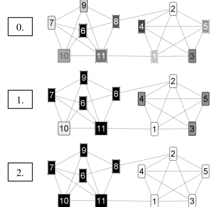
Intuitively, the algorithm works as follows in a bottom-up fashion: First, all nodes get different classes. Then the nodes are processed for a small number of iterations and inherit the strongest class in the local neighborhood. This is the class whose sum of edge weights to the current node is maximal. In case of multiple strongest classes, one is chosen randomly. Regions of the same class stabilize during the iteration and grow until they reach the border of a stable region of another class. Note that classes are updated immediately: a node can obtain classes from the neighborhood that were introduced there in the same iteration.
Figure 2 illustrates how a small unweighted graph is clustered into two regions in three iterations. Different classes are symbolized by different shades of grey.
Figure 2: Clustering an 11-nodes graph with CW in two iterations
It is possible to introduce a random mutation rate that assigns new classes with a probability decreasing in the number of iterations as described in (Biemann & Teresniak 2005). This showed having positive effects for small graphs because of slower convergence in early iterations.
The CW algorithm cannot cross component boundaries, because there are no edges between nodes belonging to different components. Further, nodes that are not connected by any edge are discarded from the clustering process, which possibly leaves a portion of nodes unclustered.
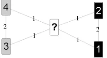
Formally, CW does not converge, as figure 3 exemplifies: here, the middle node’s neighborhood
0.
1.
consists of a tie which can be decided in assigning the class of the left or the class of the right nodes in any iteration all over again. Ties, however, do not play a major role in weighted graphs.
Figure 3: The middle node gets the grey or the black class. Small numbers denote edge weights.
Apart from ties, the classes usually do not change any more after a handful of iterations. The number of iterations depends on the diameter of the graph: the larger the distance between two nodes is, the more iterations it takes to percolate information from one to another.
The result of CW is a hard partitioning of the given graph into a number of partitions that emerges in the process – CW is parameter-free. It is possible to obtain a soft partitioning by assigning a class distribution to each node, based on the weighted distribution of (hard) classes in its neighborhood in a final step.
The outcomes of CW resemble those of Min-Cut (Wu & Leahy 1993): Dense regions in the
graph are grouped into one cluster while sparsely connected regions are separated. In contrast to
Min-Cut, CW does not find an optimal hierarchical
clustering but yields a non-hierarchical (flat) partition. Furthermore, it does not require any threshold as input parameter and is more efficient.
Another algorithm that uses only local contexts for time-linear clustering is DBSCAN as, described
in (Ester et al. 1996), needing two input parameters (although the authors propose an interactive approach to determine them). DBSCAN is especially suited for graphs with a geometrical interpretation, i.e. the objects have coordinates in a multidimensional space. A quite similar algorithm to CW is MAJORCLUST (Stein & Niggemann 1996), which is based on a comparable idea but converges slower.
2.2 Chinese Whispers as matrix operation As CW is a special case of Markov-Chain-Clustering (MCL) (van Dongen, 2000), we spend a few words on explaining it. MCL is the parallel simulation of all possible random walks up to a
finite length on a graph G. The idea is that random walkers are more likely to end up in the same cluster where they started than walking across clusters. MCL simulates flow on a graph by repeatedly updating transition probabilities between all nodes, eventually converging to a transition matrix after k steps that can be interpreted as a clustering of G. This is achieved by alternating an expansion step and an inflation step. The expansion step is a matrix multiplication of MG with the current transition matrix. The inflation step is a column-wise non-linear operator that increases the contrast between small and large transition probabilities and normalizes the column-wise sums to 1. The k matrix multiplications of the expansion step of MCL lead to its time-complexity of O(k⋅n²).
It has been observed in (van Dongen, 2000), that only the first couple of iterations operate on dense matrices – when using a strong inflation operator, matrices in the later steps tend to be sparse. The author further discusses pruning schemes that keep only some of the largest entries per column, leading to drastic optimization possibilities. But the most aggressive sort of pruning is not considered: only keeping one single largest entry. Exactly this is conducted in the basic CW process. Let maxrow(.) be an operator that
operates row-wise on a matrix and sets all entries of a row to zero except the largest entry, which is set to 1. Then the algorithm is denoted as simple as this:
D0 = In
for t=1 to iterations Dt-1 = maxrow(Dt-1) Dt = Dt-1AG
Figure 4: Matrix Chinese Whispers process. t is time step, In is the identity matrix of size n×n, AG is the adjacency matrix of graph G.
By applying maxrow(.), Dt-1 has exactly n
non-zero entries. This causes the time-complexity to be dependent on the number of edges, namely O(k⋅|E|). In the worst case of a fully connected
graph, this equals the time-complexity of MCL. A problem with the matrix CW process is that it does not necessarily converge to an iteration-invariant class matrix D, but rather to a pair of oscillating class matrices. Figure 5 shows an example.
1
1 1
1
Figure 5: oscillating states in matrix CW for an unweighted graph
This is caused by the stepwise update of the class matrix. As opposed to this, the CW algorithm as outlined in figure 1 continuously updates D after
the processing of each node. To avoid these oscillations, one of the following measures can be taken:
• Random mutation: with some probability, the
maxrow-operator places the 1 for an otherwise unused class
• Keep class: with some probability, the row is
copied from Dt-1 to Dt
• Continuous update (equivalent to CW as
described in section 2.1.)
While converging to the same limits, the continuous update strategy converges the fastest because prominent classes are spread much faster in early iterations.
3 Experiments with synthetic graphs
The analysis of the CW process is difficult due to its nonlinear nature. Its run-time complexity indicates that it cannot directly optimize most global graph cluster measures because of their NP-completeness (Šíma and Schaeffer, 2005). Therefore we perform experiments on synthetic graphs to empirically arrive at an impression of our algorithm's abilities. All experiments were conducted with an implementation following figure 1. For experiments with synthetic graphs, we restrict ourselves to unweighted graphs, if not stated explicitly.
3.1 Bi-partite cliques
A cluster algorithm should keep dense regions together while cutting apart regions that are sparsely connected. The highest density is reached in fully connected sub-graphs of n nodes, a.k.a. n-cliques. We define an n-bipartite-clique as a graph
of two n-cliques, which are connected such that each node has exactly one edge going to the clique it, does not belong to.
Figures 5 and 6 are n-partite cliques for n=4,10.
Figure 6: The 10-bipartite clique.
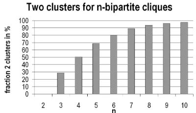
We clearly expect a clustering algorithm to cut the two cliques apart. As we operate on unweighted graphs, however, CW is left with two choices: producing two clusters or grouping all nodes into one cluster. This is largely dependent on the random choices in very early iterations - if the same class is assigned to several nodes in both cliques, it will finally cover the whole graph. Figure 7 illustrates on what rate this happens on n-bipartite-cliques for varying n.
Figure 7: Percentage of obtaining two clusters when applying CW on n-bipartite cliques
It is clearly a drawback that the outcome of CW is non-deterministic. Only half of the experiments with 4-bipartite cliques resulted in separation. However, the problem is most dramatic on small graphs and ceases to exist for larger graphs as demonstrated in figure 7.
3.2 Small world graphs
A structure that has been reported to occur in an enormous number of natural systems is the small world (SW) graph. Space prohibits an in-depth
arbitrary nodes. Steyvers and Tenenbaum (2005) show that association networks as well as semantic resources are scale-free SW-graphs: their degree
distribution follows a power law. A generative model is provided that generates undirected, scale-free SW-graphs in the following way: We start with a small number of fully connected nodes. When adding a new node, an existing node v is chosen with a probability according to its degree. The new node is connected to M nodes in the neighborhood of v. The generative model is parameterized by the number of nodes n and the network's mean connectivity, which approaches 2M for large n.
Let us assume that we deal with natural systems that can be characterized by small world graphs. If two or more of those systems interfere, their graphs are joined by merging some nodes, retaining their edges. A graph-clustering algorithm should split up the resulting graph in its previous parts, at least if not too many nodes were merged.
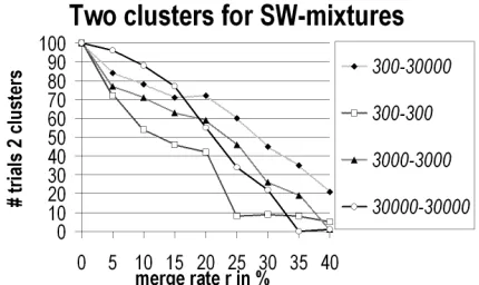
We conducted experiments to measure CW's performance on SW-graph mixtures: We generated graphs of various sizes, merged them by twos to a various extent and measured the amount of cases where clustering with CW leads to the reconstruction of the original parts. When generating SW-graphs with the Steyvers-Tenenbaum model, we fixed M to 10 and varied n and the merge rate r, which is the fraction of nodes of the smaller graph that is merged with nodes of the larger graph.
Figure 8: Rate of obtaining two clusters for mix-tures of SW-graphs dependent on merge rate r.
Figure 8 summarizes the results for equisized mixtures of 300, 3,000 and 30,000 nodes and mixtures of 300 with 30,000 nodes.
It is not surprising that separating the two parts is more difficult for higher r. Results are not very
sensitive to size and size ratio, indicating that CW is able to identify clusters even if they differ considerably in size – it even performs best at the skewed mixtures. At merge rates between 20% and 30%, still more then half of the mixtures are separated correctly and can be found when averaging CW’s outcome over several runs.
3.3 Speed issues
As formally, the algorithm does not converge, it is important to define a stop criterion or to set the number of iterations. To show that only a few iterations are needed until almost-convergence, we measured the normalized Mutual Information (MI)1 between the clustering in the 50th iteration and the clusterings of earlier iterations. This was conducted for two unweighted SW-graphs with 1,000 (1K) and 10,000 (10K) nodes, M=5 and a weighted 7-lingual co-occurrence graph (cf. section 4.1) with 22,805 nodes and 232,875 edges. Table 1 indicates that for unweighted graphs, changes are only small after 20-30 iterations. In iterations 40-50, the normalized MI-values do not improve any more. The weighted graph converges much faster due to fewer ties and reaches a stable plateau after only 6 iterations.
Iter 1 2 3 5 10 20 30 40 49 1K 1 8 13 20 37 58 90 90 91 10K 6 27 46 64 79 90 93 95 96 7ling 29 66 90 97 99.5 99.5 99.5 99.5 99.5
Table 1: normalized Mutual Information values for three graphs and different iterations in %.
4 NLP Experiments
In this section, some experiments with graphs originating from natural language data are presented. First, we define the notion of co-occurrence graphs, which are used in sections 4.1 and 4.3: Two words co-occur if they can both be found in a certain unit of text, here a sentence. Employing a significance measure, we determine whether their co-occurrences are significant or random. In this case, we use the log-likelihood measure as described in (Dunning 1993). We use the words as nodes in the graph. The weight of an
1 defined for two random variables X and Y as
edge between two words is set to the significance value of their co-occurrence, if it exceeds a certain threshold. In the experiments, we used sig-multilingual corpus by languages, assuming its tokenization in sentences.
The co-occurrence graph of a multilingual corpus resembles the synthetic SW-graphs: Every language forms a separate co-occurrence graph, some words that are used in more than one language are members of several graphs, connecting them. By CW-partitioning, the graph is split into its monolingual parts. These parts are used as word lists for word-based language identification. (Biemann and Teresniak, 2005) report almost perfect performance on getting 7-lingual corpora with equisized parts sorted apart as well as highly skewed mixtures of two languages.
In the process, language-ambiguous words are assigned to only one language, which did not hurt performance due to the high redundancy of the task. However, it would have been possible to use the soft partitioning to acquire a distribution over languages for each word.
4.2 Acquisition of Word Classes
For the acquisition of word classes, we use a different graph: the second-order graph on neighboring co-occurrences. To set up the graph, a co-occurrence calculation is performed which yields significant word pairs based on their occurrence as immediate neighbors. This can be perceived as a bipartite graph, figure 9a gives a toy example. Note that if similar words occur in both parts, they form two distinct nodes.
This graph is transformed into a second-order graph by comparing the number of common right
and left neighbors for two words. The similarity (edge weight) between two words is the sum of common neighbors. Figure 9b depicts the second-order graph derived from figure 9a and its partitioning by CW. The word-class-ambiguous word “drink” (to drink the drink) is responsible for all intra-cluster edges. The hypothesis here is that words sharing many neighbors should usually be observed with the same part-of-speech and get high weights in the second order graph. In figure 9, three clusters are obtained that correspond to different parts-of-speech (POS).
(a) (b)
Figure 9: Bi-partite neighboring co-occurrence graph (a) and second-order graph on neighboring co-occurrences (b) clustered with CW.
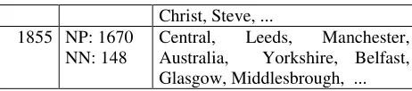
To test this on a large scale, we computed the second-order similarity graph for the British National Corpus (BNC), excluding the most frequent 2000 words and drawing edges between words if they shared at least four left and right neighbors. The clusters are checked against a lexicon that contains the most frequent tag for each word in the BNC. The largest clusters are presented in table 2 .
size tags:count sample words
18432 NN:17120 AJ: 631
secret, officials, transport, unemployment, farm, county, wood, procedure, grounds, ...
Christ, Steve, ... 1855 NP: 1670
NN: 148
Central, Leeds, Manchester, Australia, Yorkshire, Belfast, Glasgow, Middlesbrough, ... Table 2: the largest clusters from partitioning the second order graph with CW.
In total, CW produced 282 clusters, of which 26 exceed a size of 100. The weighted average of cluster purity (i.e. the number of predominant tags divided by cluster size) was measured at 88.8%, which exceeds significantly the precision of 53% on word type as reported by Schütze (1995) on a related task. How to use this kind of word clusters to improve the accuracy of POS-taggers is outlined in (Ushioda, 1996).
4.3 Word Sense Induction
The task of word sense induction (WSI) is to find the different senses of a word. The number of senses is not known in advance, therefore has to be determined by the method.
Similar to the approach as presented in (Dorow and Widdows, 2003) we construct a word graph. While there, edges between words are drawn iff words occur in enumerations, we use the co-occurrence graph. Dorow and Widdows construct a graph for a target word w by taking the sub-graph induced by the neighborhood of w (without w) and clustering it with MCL. We replace MCL by CW. The clusters are interpreted as representations of word senses.
To judge results, the methodology of (Bordag, 2006) is adopted: To evaluate word sense induction, two sub-graphs induced by the neighborhood of different words are merged. The algorithm's ability to separate the merged graph into its previous parts can be measured in an unsupervised way. Bordag defines four measures:
• retrieval precision (rP): similarity of the
found sense with the gold standard sense
• retrieval recall (rR): amount of words that
have been correctly assigned to the gold standard sense
• precision (P): fraction of correctly found
disambiguations
• recall (R): fraction of correctly found
senses
We used the same program to compute co-occurrences on the same corpus (the BNC). Therefore it is possible to directly compare our
results to Bordag’s, who uses a triplet-based hierarchical graph clustering approach. The method was chosen because of its appropriateness for unlabelled data: without linguistic pre-processing like tagging or parsing, only the disambiguation mechanism is measured and not the quality of the preprocessing steps. We provide scores for his test 1 (word classes separately) and test 3 (words of different frequency bands). Data was obtained from BNC's raw text; evaluation was performed for 45 test words.
% (Bordag, 2006) Chinese Whispers POS P R rP rR P R rP rR N 87.0 86.7 90.9 64.2 90.0 79.5 94.8 71.3
V 78.3 64.3 80.2 55.2 77.6 67.1 87.3 57.9
A 88.6 71.0 88.0 65.4 92.2 61.9 89.3 71.9 Table 3: Disambiguation results in % dependent on word class (nouns, verbs, adjectives)
% (Bordag, 2006) Chinese Whispers freq P R rP rR P R rP rR high 93.7 78.1 90.3 80.7 93.7 72.9 95.0 73.8
med 84.6 85.2 89.9 54.6 80.7 83.8 91.0 55.7
low 74.8 49.5 71.0 41.7 74.1 51.4 72.9 56.2 Table 4: Disambiguation results in % dependent on frequency
Results (tables 3 and 4) suggest that both algorithms arrive at about equal overall performance (P and R). Chinese Whispers clustering is able to capture the same information as a specialized graph-clustering algorithm for WSI, given the same input. The slightly superior performance on rR and rP indicates that CW leaves fewer words unclustered, which can be advantageous when using the clusters as clues in word sense disambiguation.
5 Conclusion
application field of CW rather lies in size regions, where other approaches’ solutions are intractable.
On the NLP data discussed, CW performs equally or better than other clustering algorithms. As CW – like other graph clustering algorithms – chooses the number of classes on its own and can handle clusters of different sizes, it is especially suited for NLP problems, where class distributions are often highly skewed and the number of classes (e.g. in WSI) is not known beforehand.
To relate the partitions, it is possible to set up a hierarchical version of CW in the following way: The nodes of equal class are joined to hyper-nodes. Edge weights between hyper-nodes are set according to the number of inter-class edges between the corresponding nodes. This results in flat hierarchies.
In further works it is planned to apply CW to other graphs, such as the co-citation graph of Citeseer, the co-citation graph of web pages and the link structure of Wikipedia.
Acknowledgements
Thanks go to Stefan Bordag for kindly providing his WSI evaluation framework. Further, the author would like to thank Sebastian Gottwald and Rocco Gwizdziel for a platform-independent GUI implementation of CW, which is available for download from the author’s homepage.
References
F. Amblard. 2002. Which ties to choose? A survey of social networks models for agent-based social
simulations. In Proc. of the 2002 SCS International
Conference On Artificial Intelligence, Simulation and Planning in High Autonomy Systems, pp.253-258, Lisbon, Portugal.
C. Biemann, S. Bordag, G. Heyer, U. Quasthoff, C. Wolff. 2004. Language-independent Methods for
Compiling Monolingual Lexical Data, Proceedings
of CicLING 2004, Seoul, Korea and Springer LNCS 2945, pp. 215-228, Springer, Berlin Heidelberg B. Bollobás. 1998. Modern graph theory, Graduate
Texts in Mathematics, vol. 184, Springer, New York S. Bordag. 2006. Word Sense Induction: Triplet-Based
Clustering and Automatic Evaluation. Proceedings of
EACL-06. Trento
C. Biemann and S. Teresniak. 2005. Disentangling from Babylonian Confusion – Unsupervised Language
Identification. Proceedings of CICLing-2005,
Mexico City, Mexico and Springer LNCS 3406, pp. 762-773
S. van Dongen. 2000. A cluster algorithm for graphs.
Technical Report INS-R0010, National Research Institute for Mathematics and Computer Science in the Netherlands, Amsterdam.
T. Dunning. 1993. Accurate Methods for the Statistics
of Surprise and Coincidence, Computational
Linguistics 19(1), pp. 61-74
M. Ester, H.-P. Kriegel, J. Sander and X. Xu. 1996. A Density-Based Algorithm for Discovering Clusters in
Large Spatial Databases with Noise. In Proceedings
of the 2nd Int. Conf. on Knowledge Discovery and Datamining (KDD'96) Portland, USA, pp. 291-316. B. Dorow and D. Widdows. 2003. Discovering
Corpus-Specific Word Senses. In EACL-2003 Conference
Companion (research notes and demos), pp. 79-82, Budapest, Hungary
R. Ferrer-i-Cancho and R.V. Sole. 2001. The small
world of human language. Proceedings of The Royal
Society of London. Series B, Biological Sciences, 268(1482):2261-2265
H. Schütze. 1995. Distributional part-of-speech
tagging. In EACL 7, pages 141–148
J. Šíma and S.E. Schaeffer. 2005. On the
np-completeness of some graph cluster measures.
Technical Report cs.CC/0506100, arXiv.org e-Print archive, http://arxiv.org/.
B. Stein and O. Niggemann. 1999. On the Nature of
Structure and Its Identification. Proceedings of
WG'99, Springer LNCS 1665, pp. 122-134, Springer Verlag Heidelberg
M. Steyvers, J. B. Tenenbaum. 2005. The large-scale structure of semantic networks: statistical analyses
and a model of semantic growth. Cognitive Science,
29(1).
Ushioda, A. (1996). Hierarchical clustering of words
and applications to NLP tasks. In Proceedings of the
Fourth Workshop on Very Large Corpora, pp. 28-41. Somerset, NJ, USA
D. J. Watts. 1999. Small Worlds: The Dynamics of
Networks Between Order and Randomness, Princeton
Univ. Press, Princeton, USA
Z. Wu and R. Leahy (1993): An optimal graph theoretic approach to data clustering: Theory and its
application to image segmentation. IEEE