Steady surface wave pattern in a shear flow

Thesis by Joseph P . Lau

In Partial Fulfillment of the Requirements For the Degree of

Doctor of Philosophy

California Institute of Technology Pasadena, California

1968

-ii-ACKNOWLEDGMENT

The author wishes to express his profoundest gratitude to Professor T. Yao-Tsu Wu for the constant guidance and supervision

given him throughout the entire course of this research. He has benefited tremendously from Professor Wu1_{s valuable criticism,} suggestions and encouragement.

The author is grateful to the California Institute of Technology for the award of Institute Scholarships, Ford Foundation Fellowships and Woodrow Wilson Fellowships during the years of his graduate study. Part of this investigation has been done under Contract Nonr 220(35) with the Office of Naval Research, Department of the Navy.

Abstract

The subject under investigation concerns the steady surface wave patterns created by small concentrated disturbances acting on a non-uniform flow of a heavy fluid. The initial value problem of a point disturbance in a primary flow having an arbitrary velocity distribution (U(y}, 0, 0) in a direction parallel to the undisturbed free surface is formulated. A geometric optics method and the clas

-sical integral transform method are employed as two different methods of solution for this problem. Whenever necessary, the

special case of linear shear (i. e. U(y)

=

U (1

+

ey) ) is chosen for the 0

purpose of facilitating the final integration of the solution.

The asymptotic form of the solution obtained by the method of integral transforms agrees with the leading terms of the solution obtained by geometric optics when the latter is expanded in powers of small Er.

The overall effect of the shear is to confine the wave field on the downstream side of the disturbance to a region which is smaller than the wave region in the case of uniform flows. If U(y)

vanishes, and changes sign at a critical plane y

=

y (e.g. er

ey

=

-1 for the case of linear shear), then the boundary of this er

Inside the wave field, as in the case of a point disturbance in a uniform primary flow, there exist two wave systems. The loci of

constant phases (such as the crests or troughs) of these wave sys-terns are not symmetric with respect to the x-axis. The geometric

optics method and the integral transform method yield the same result of these loci for the special case of U(y)

=

U (1

+

E y) and for

0 large K r ( E r

«

1

« K

r ) .

Chapter

I. II.

III.

IV.

V.

· Table of Contents

Page

Acknowledgment ii

Abstract iii

Introduction 1

General Formulation 7

'

1. Co-ordinate system and convention 7

2. Equations of motion 7

3. Boundary conditions 8

4. Linea:i:-ization 9

5. Review of steady wave pattern in a uniform

flow i 2

Method of Geometric Optics 1. Unsteady problem

2. Steady wave pattern 3. A perturbation expansion Integral Transform Method Discussion and Conclusion References

Figures Appendices

17 17 27

36

46

I. INTRODUCTION

In oceanography, the effects of strongly sheared ocean

cur-rents on the propagation of ocean waves present problems of

consider-able interest. Another example of water waves in shear flow is the

ship waves propagating in the wake and near the stern of a ship. A

steady wave pattern of surface wave is produced by a concentrated

stationary disturbance located either on the surface or submerged within a steady primary shear flow. This class of problems

is of basic academic interest as well as of great importance in ship

hydrodynamics because it can predict the main features of the system

of waves accompanying a ship moving through a sufficiently deep water.

There exists an extensive literature concerning the special

case when the primary flow is uniform. The classical method of

solution is discussed in Lamb's Hydrodynamics (Ref. 7) where applica -tion is made to gravity waves (Kelvin's ship wave-pattern) in §256 and to capillary and combined capillary-gravity waves in §272. The ex -tension of this classical. method to disturbances of variable or pulsat-ing strength and following an arbitrary path in a uniform primary flow

may be found in Wehausen and Laitone (Ref. 18) and Stoker (Ref. 14).

In contrast, the problem is much more difficult when the

primary flow is non-uniform. Several papers treating the problems of disturbances in a rotational flow are limited to two dimensional dis

lines in these flows are straight, remain parallel to one another, and

are not stretched during the motion. Hence they are relatively

easy to treat.

When the disturbance is three-dimensional, even though the undisturbed flow may still be unidirectional and does not possess a free surface, the stretching and bending of vortex lines must play an

important role. Certain outstanding papers on the theory of these

flows have appeared.

A basic theorem that two-dimensional disturbances become

unstable at a lower critical Reynolds number than three -dimensional disturbances has been given by Squire (Ref. 12 ).

Squire and Winter (Ref. 13) have investigated steady three-dimensional disturbances to a parallel shear flow with no free surface

by the so-called "secondary flow" method. In this treatment, no

restriction is placed on the disturbances but there is an assumption that the undisturbed stream is weakly sheared. The shear is usually

taken to be linear though this is not an essential limitation to the method. A difficulty arising in the application of this theory is that

the secondary flow disturbance due to the presence of an obstacle falls

off more slowly with distance than does the primary flow disturbance. This limits the validity of the solution to the region near the obstacle.

In an effort to clear up this difficulty Lighthill (Ref. 9) has studied the fundamental solution of a small steady three -dimensional disturbance in a two-dimensional parallel shear flow without a free

that the small perturbation theory based on neglecting the squares of

the perturbation velocities u, v and w is valid far from the obstacle

and overlaps the region where the secondary flow solution is valid.

The asymptotic behavior of this solution for large r shows that a

source in a shear layer produces in a region of uniform flow outside

the shear layer a disturbance equivalent to a source of different

strength at a different position. The strength of the equivalent source

can be predicted by an image method in which the shear layer is

rega:rded as a superposition of layers of piecewise uniform flows. The

displacement ineffective position is of the order of the width of the shear

layer. It is expected that such modification of source strength and

position will no longer be so simple in the presence of a free surface.

In fact, in the presence of a free surface, the difficulties of

treating the stretching and bending of the vortex lines are further en-hanced. If the undisturbed flow contains a vortex sheet i.e. a dis -continuity in velocity, perpendicular to the free surface, any

disturb-ance rnay produce wave motions both in the free surface and in the

vortex sheet. Development of a theory de scribing the interaction be

-tween the waves and these free surfaces is a difficult mathematical

task. For primary flows having a continuous horizontal velocity

distribution, the free surface waves produced by an obstacle will de-finitely be affected by the vorticity of the primary flow.

In spite of the difficulties described above, Ursell (Ref. 17)

irrotational and does not vary rapidly with distance, he has developed

a theory, for the steady wave pattern, based on the following assump-tions:

(i) The streaming velocity component normal to a

wave crest is equal to the phase velocity based

on the local wave length;

(ii) the separation between consecutive crests is

equal to the local wave length.

The purpose of the present study is to develop systematically

a theory for steady surface wave patterns due to a small concentrated

disturbance in a primary parallel rotational flow. In the construction of the phase curves by Ursell (reference 1 7) it was assumed that the

phase velocity relative to a si.ightly non-uniform stream of variable depth can be adequately approximated by the phase velocity obtained from constant depth theory. The validity of this implicit assumption

of adopting the original dispersion relationship for uniform flows of constant depth for rotational non-uniform primary flows is not im-mediately obvious. Indeed, our theory shows that if terms other

than the two lowest orders are kept, this is no longer valid.

By discarding the squares of the perturbation velocities u, v

and w of the velocity field (U(y)

+

u, v, w), we shall first formulate the problem for an arbitrary primary parallel shear flow U(y} with

an undisturbed free surface at z

=

0, in Chapter II.

A method based on the notion of group velocity and geometric

by Keller (reference 6) and by others, is applied to the problem of a small stationary concentrated surface disturbance on a primary parallel shear flow U(y) in Chapter III. In section 1, U(y) is kept arbitrary but in sections 2 and 3, solution for the special case of

U(y) = U (1

+

e y) is carried out while no restriction is placed on e 0

It is believed that the true behavior of the flow far from the disturb-ance must be obtained from the full equations with the squares of the disturbance neglected. Such an approach results in a 11

small-perturbation11 _{solution. The region of validity of this result is at} large distances from the disturbance and overlaps the region near the disturbance where a '1_{small- shear}11 _{solution is valid. This} over-lapping holds in the sense that the asymptotic behavior of the 11_small shear11

solution is sim:.lar to the asymptotic behavior of a perturba-. -ti on expansion of the 11 _{small-perturbation}11 _{solution for small er.} This is, indeed, indicated by comparison of the results of

Chapter III, section 3, and Chapter IV.

The geometric optics method of Chapter III fails at the bound-ary of the wave region. For the special case of uniform primary flow, Ursell (reference 16) has determined the behavior of the waves near the boundary of the wave region by a modification of the prin-ciple of stationary phase. Thus showing that for dispersive waves, the integral transform method is the fundamental one. Therefore, in Chapter IV, we shall modify the classical integral transform method to treat a weak submerged source of constant strength in a primary linear shear flow, i.e. U

=

U

11_{secondary flow'' method, we take the "primary flow" to coincide}

with that in which the undisturbed stream is uniform and the

"secondary flow" to be a perturbation of the primary flow by allowing

a small shear ( e small) in the undisturbed stream. The resulting

"small shear" solution, obtained by applying the method of

stationary phase to evaluate the inverse transform, is valid for

1

large r (<-). However, a more elaborate asymptotic technique E

will have to be applied in order to deduce a solution valid near the

boundary of the wave region.

Although the velocity distribution U (1

+e

y) considered in 0

Chapter III and Chapter IV may seem somewhat artificial, it

never-theless provides some insight to the problem of arbitrary U(y) as

well as a first approximation to the horizontal velocity distribuUon

of the ocean near the shore-line. In the present treatment, surface

tension and viscous terms in the equations are neglected. This is

known to be permissible except near the critical region where U(y)

is zero. Accordingly the theory developed here is limited to a region

II. GENERAL FORMULA TI ON

1. Co-ordinate system and convention

The problem in question concerns the propagation of surface

waves in a body of heavy fluid, of infinite depth, initially having a pre

-scribed non-uniform horizontal velocity distribution, due to a

station-ary disturbance. The fluid is taken to be inviscid and incompressible,

of constant density p. The resulting flow will be generally rotational;

the disturbance is however assumed to be so small that a linear theory

can be applied. Consider a righthanded rectilinear coordinate sys

-tern such that (Fig. 1 )

(i) the z -axis points vertically :ipward, with z

=

0

coinciding with the undisturbed free surface, and the

grav-ity acting in the negative z -direction;

(ii) the x-axis is in the direction of the undisturbed stream

which is taken to be a function of y only; and

(iii) the y-axis completes the system.

The x, y, z-components of the velocity vector q are denoted by u, v,

w, the pressure by p, the density by p and the gravitational accel-eration by g. Other notations will be defined in the text as needed.

2. Equations of motion

The primary flow is unidirectional and has a prescribed shear

given by

q

0

=

(U(y), 0, 0)

Po

= -pgz

where U(y) is an arbitrary function of y and is assumed to be at

least twice differentiable. With q,:, and p>:, representing the total

veloc-ity vector and pressure respectively, the momentum equation for an

inviscid, incompressible flow is

8q,:c

~

+

(q,:: \i' )q>!,

The continuity equation is

\i'

P

,:,

= -

- -

-Y'gz p

'V·q,;,

=

Q(x, t),

where Q(x, t) represents a source in the fluid.

3. Boundary conditions

(2. 2)

(2. 3)

The boundary conditions on the free surface of the heavy fluid

can be stated as follows. Let the free surface be Sf: z -

t;

(x, y, t) = 0

where

t;,

(x , y, t) is the vertical displacement of the free surface meas

-ured from z = 0. The dynamic condition of constant pressure at the

free surface required

=

0 on z=t;,(x,y,t) (2. 4)

The kinematic condition for the particles on the free surface is

z=t;,(x,y,t) (2. 5)

On solid surfaces with specified shapes S(x, y, z, t) = 0 the boundary

condition is

4. Linearization

The flow field maybe considered as a combination of the pr ima-ry shear flow (q

0 , p0 } and a perturbation (q , p) so that

q,:,

=

q

0

+

q

=

(U(y)

+

u,v,w}, (2. 7)

p .._.,, .

=

p ₀

+

p

= -

pgz

+

p

If the departure from the primary flow is small, then by neglecting

the squares and products of u,v,w and their derivatives, Eqs. (2.2),

(2. 3) can be linearized to give

Du+ U'(y}v

+

_{a: {}

~

)

=

o

'

Dv

+

~

ay

(

E.

_p

)

=

0 _,

Dw

+

a:

{

~

)

=

_0'

au

+

av

+

8w

=

Q(x, t)

ax

ay

8Z

-

a

where D

=

8t

+

_{U (y)}

ax'

a

and in the sequel D'

=

U' (y)

ax

8 and (2. 9) (2. 1 0)

(2. 11 )

(2. 12)

D" :: U"(y)

0: The linearized free surface conditions can be readily

shown to be

-pgw

+

Dp

=

0 (2.13)

D

s

=

w

whereas the boundary condition on solid surface remains unchanged.

Elimination of p by cross differentiations of (2. 9), (2. 10) and (2. 11) gives

a

a

oy

Dw

=

D

az

av

(2.16)

Although from (2. 12), (2.15) and (2.16) a single equation for any

component of the perturbation velocity q

=

(u, v, w} can be obtained,

the equation with v as the dependent variable is preferred. By

eliminating u and w, we obtain

[ DV'2 - D"] v =

0

~

DQ(x, t) (2. 1 7)

Equation (2. 1 7) is the basic equation of motion. When v has been

solved together with appropriate boundary conditions, u and w may

be deduced from (2. 16) and the continuity equation. To obtain w, the

lower limit in the y-integral may be taken as either +«:> or -oo since

the disturbances are assumed to vanish at both limits. The result

obtained using either limit is the same. In integrating the continuity

equation with respect to x to obtain u, however, the lower limit

must be -oo because it is possible that the fluid at +«:> in which

region the vorticity may be permanently changed after the fluid has

passed the disturbance, may not have zero disturbance velocity i. e.

we shall only assume all disturbances vanish farup stream (at x

=

-oo ).

The appropriate condition on the free surface for v can be

derived by differentiating (2. 13) giving

-g

~

oy

Dw

+

~

D2 {

E.)

= 0

By

p (2.18)

Eliminating w from (2. 18) and (2. 16), we obtain after som e manip

- g ₈8z Dv + D2

8

~

(

~)

+ 2DD' (

~)

=

o

By using (2. 10) in the second term and integrating the resulting

equa-tion once, we have

- g ov - D2v + 2D'(

E.)

=

0

8z p (2. 19)

Recalling D'

=

U'(y)

:x,

Eq. (2.9) can be used to

eliminate(~),

yielding

+ g

~~

+

D2v + 2U1_{(y)(Du + U '(y)v )}

=

_{0 (2 .. 20)}

Finally,dividing(2.20)by U'(y), differentiatingitwithrespectto y, then

using (2. 15) to eliminate u, we obtain the free surface boundary

condition as

{

z

8v}

a

Dv+gaz

e

8y U I

(y

)

= -

2 8x Dv on z=O • (2.21)

With appropriate initial and boundary conditions, v can be solved from

(2.17)and(2.21). Sofarnorestrictionhasbeenplacedon U(y). They

are linear partial differential equations with variable coefficients

which depend on y in such a complicated manner that it is quite

dif-ficult to obtain an analytical solution for the general case of arbitrary

U(y). In Chapter III a geometric optics method will be developed for

the case when the variation of U(y), otherwise arbitrary, is as

-sumed small. In Chapter IV an integral transform method will be

applied to solve (2. 17) and (2. 21) for v for a particular, although

somewhat artificial U(y), namely that of linear shear,

u (y)

=

u ( 1

+ ~y)

It is obvious that this type of undisturbed parallel velocity distribution,

if exists at all, is rare. Nevertheless the solution may give some

in-sight to the much harder problem of arbitrary U(y).

5. Review of steady wave pattern in a uniform stream

The treatment of a stationary point source of strength m,

sub-merged in a uniform primary flow, by double Fourier transform and

asymptotic evaluation of certain integrals based on the principle of

stationary phase illustrates the characteristic difficulties involved

(Ref.18 ). We shall review this method briefly to fix ideas as well as

for discussion and comparison of the results with the case in which the

primary flow is non-uniform.

Let rectangular cartesian co-ordinates (x, y, z) be chosen with

the z -axis perpendicular to the undisturbed free surface, the x-axis

parallel to the stream velocity U,

0 and the y-axis completing the system. The gravity acts in the negative z-direction, with

gravitation-al acceleration g.. The origin is taken so that the point of disturbance is at (0, 0, - h). Polar co-ordinates (r,

a, z) are defined by

x

=

r cos

a,

y

=

r sin

a.

Our problem is to find the velocity potential

cp (x, y, z) based on the linearized theory that in the flow field z

<

0,

0

cf> satisfies the Laplace equation 0

\72cp

=

0

0 except at (0,0, -h)

and the boundary condition at the free surface z = 0 that

(z

=

0)

(2. 23)

where K

=

g/U 2 is a characteristic wave number. We further write 0

m 1 ...,

q,

o (x' y' z )

=

-

4n

R

+

cf> (x' y' z) '

l

where

¢'

is a harmonic function, regular in the region z

<

0, and

Rz

=

xz + yz + (z+h)z

l

For the condition at infinity we require

lim grade/> = 0

0

z-+ -oo

lim grade/> = 0

(\ x-> -oo

Applying the double Fourier Transform,defined as

J{c/>)

=

s

oo dx

s

oo dy ;i(ax+f3 y )cf> o

. -IX> -00

(2.25)

(2. 26)

(2. 27)

(2. 28)

to (2. 23 ), we obtain a second order ordinary differential equation with

z as the only independent variable. The coefficients in the solution of

this transformed equation are determined by the transform of the

bound-ary conditions. The details of the method of solution can be found in

Havelock (Ref. 4 ) and elsewhere and will not be repeated here. With

the notatic:n

a = k cos

e

(2. 29)

f3

=

k sine

cb

(x, y, z)

0

m 1 m 1

=

-

4TI"

R

+

4ir

R

1

z

'IT

+Re 1 ('

2

dB

s

00 dkeikr cos(B-a)ek(z-h) mK secie ,

2'ITZ

j

'IT o k-K secZB

(2. 3 0)

where Rz

=

xz

+

yz +(z-h)z and "Re" denotes 11_{the real part of". The}

z

physical significances of the terms on the right-hand side of (2. 30),

are respectively, the point source, its reflection into the plane z

=

0,

and thE.: disturbance due to the free surface effects, including the sur

-face waves. By evaluating the k·-integral along an appropriate path, the

integral in (2. 30), for cos(B-a)

>

0, yields in the final result of

cb

a

0

term of the following integral representation

e

i

j

'

·

7 da eirK secze cos(B-a) K seczB(z-h} za

Re 17 e mK sec 17

'IT

e

where

e

and for O"

~

0

+

O"

This integral is in suitable form for the application of the method of

stationary phase. F or large Kr and for each particular a, the

sta-tionary points are given by the roots of

~

[ secze cos(B-a )]

=

0

or

Explicitly, there are two roots 8

tan

e

=

±

and

e

+' given by

-1±

J

1 -8 tan2cr

4 tancr (2. 32)

The asymptotic form of the wave part of cf>

0 for large Kr follows from the principle of stationary phase to give

{ 2.

_1T4}

c/>

0

=

- A(8+)sin rKsece+ cos(8+-a)+

-A(8_)sin+K sec28_cos(8_-a) -

~}

(2.33)

where

[ .

-·- ( 1+4 tan 2 8±)

1/

4 A(8 _± ) -_{_}

_z

_rn

_

_{mK sec ±}

e

I

( 1-2 tan2

e

±)1 2.

(2. 34)

with 8 given by (2. 32). The above results show that the resultant

±

wave pattern of a subrnerged source is the superposition of two sys

-terns of wave which are confined in the wedge bo'..1nded by two vertical

planes

a

= ±

a_.

_....

_

~

,

a_,_

.. ,~ = 19. 5°. The general features of the curves of constant phase are shown in Fig. Sb.

The variation of the amplitude is indicated by Eq. (2. 34). The

above expressions (2. 33) and (2. 34) break down when the second

deriv-ative of the phase function sec28 cos(8-cr) with respect to

e

vanishes;

this occurs at the boundary

a

= ±a,:, of the wave region. By a more

elaborate asymptotic method, Ur sell ( 16) has shown that the leading

1

term of cf>

0 is of order O(Kr

)-3 _{in the region near la}

I

₌

I

_a,:,

I

.

_In

this region, the m ethod of geometric optics to be discussed in Chapter

phase therefore seems more fundamental. But it can be seen that

this integral transform method, without modifications, fails when the

primary flow is non-uniform because Eqs. (2. 23) and (2. 24) are

re-placed by Eqs. (2. 17) and (2. 21) which have variable coefficients. We

shall show in Chapter IV, how this integral transform approach can be

Ill. METHOD OF GEOMETRIC OPTICS

1. Unsteady problem

The method of geometric optics has been developed and applied

to problems involving wave motions in anisotropic and dispersive

media by Landau and Lifshitz ( 8 ), Lighthill ( 10), Whitham ( 20),

Keller ( 6 ), and by others. The basic assumption necessary for

sue-cessfu1_{. application of this method is that the non-uniformity in the}

dispersive medium in which the wave propagates does not change

sig-nificantly over distances comparable to the typical wave-length under

consideration. In our present problem of gravity waves, in a parallel

shear stream with free stream velocity U(y), this assumption may be

interpreted as

u

2

I

gP.

«

1 0

where U

0 is a characteristic constant velocity, U 0

2

I

_{g , is the typical}

wave length, and l is a characteristic length over which the primary

parallel shear flow velocity, changes appreciably. For example, l

may be chosen to be U

I

(mean value of !du

I

dy

I )

.

In this section, the 0

problem of a point disturbance applied on the surface of the fluid at

x

=

0, y

=

0 for t

>

0 is fir st formulated. The steady wave pattern

due to a stationary point disturbance on the surface is then deduced

quite readily.

We consider here a general distribution of velocity U(y),

U(y)

=

U

+ U

(y)

0 l (3. 1 )

small compared to U . When the variations of U(y) are smooth, we

0

can keep a clear separation between the phase of a surface wave and

its amplitude. Thus we may write

~ ~ i</> (x t) ~

v(x, t)

=

A(x, t)e '

=

A exp{i</>(x, t)

+

L(x, t)}

0 (3. 2)

where

L(x, t)

=

log[

A(;,

t)/ A ]

0

and A is a reference amplitude, A(x, t) is the amplitude function,

0

which is assumed to be slowly varying in x and t. The function

<f>(x t) in general may be complex, its imaginary part is determined by the differential equation goverr..i~g v. To represent a surface wave,

the real part of cf> as sum es the for:rri

Re{cf> (;, t)} = k

l\J (;,

t) = k '1r(x, t) - wt

0 0 (3. Za)

where k is a constant reference wave number appropriate to the wave

0

motion in question, w

=

w(x, t) is the circular frequency, and the real

function '1r(x, t) is the so-called eikonal function, which defines the

surfaces of equal phase.

For the geometric wave approximation we next introduce the

basic assumption that the characteristic wavelength Zn /k is assumed

0

to be small compared to the distance 1 over which U(y) changes

ap-preciably. Hence, if x is referred to l , and t to k l/w , as the

0 0

basic units, then from the above assumption it follows that the

[gradcp

I

=

O(k .l)

0

(3. 3)

lgr_ad

LI

=

0(1)

and the higher order derivatives of cf> with respect to x and t are

clearly also of order (k i). Since the geometric wave approximation

0

requires k I. to be large, the differential equations for cf> and L can

0

be derived by substituting v into the basic equation of motion (2. l 7)

and the boundary condition (2. 21 ), then expanding the equations for

small (1/k 1). Consequently, the terms in (2. 17) have the following

0

orders of magnitude:

IU11

v _x I

=

O(IU"vl(k 1) )

0

where the prime denotes differentiation with respect to y, as before.

Hence, up to the first two leading terms for k 1 large, we have

0

which holds true for arbitrary U(y) provided the variation of U(y) is

smooth, a factor of error

equation being under stood.

[l+O(k l)-2] for the left side of the above

0

This equation can be integrated once,

giv-ing "V2v

=

f(x - Ut), f(x) being an arbitrary function of x; but this

function must be zero since '\flv is required to vanish as y2

+

zz.-+ oo

in the flow field. Whence

\lz.v

=

0 (3. 4)

valid for the first two leading orders. The free surface condition (2. 21)

(3. 5)

It may be noted that the two terms on the left hand side of (3. 5) may be

regarded to be of the same order since the parameter gl/ U ~ , which

is the factor multiplying v

z in the dimensionless form of the equation,

can be very large. It is also noted that the terms on the right hand side

of (3. 5) enter in the calculation of the second order term.

By substituting (3. 2) into (3. 4) and retaining only the two

lead-ing orders, we obtain

and

2 (

ocb o

L

+

ocb o

L -1..

ocb o

L)

+

o

2

:/J

o

2ef>

ox ox

oy oy

·

az

oz

axz.

+

oyz.

From (3. 6),

i

oc/l

az

(3. 6)

=

0 (3. 7)

(3. 8)

Hence we observe that if the partial derivatives of

cp

with respect to x and y are real, as is required by the solution representing a

sur-face wave propagating in the x-y plane, then

oc/>/oz

will be purely

imaginary so that v will vary exponentially with respect to z. In

1

(3.6), an appropriate branch of the function (cf> z

+</>

2

)2 is chosen to

x y

satisfy the boundary condition that v --+ 0 as z --+ - oo. By

differentiat-ing (3. 6) with respect to x, y, z, and by some substitutions, we find

ocp aq, o

2

cp

+

(

ocp

}

2

o

2

cp }

By making use of (3.8) and (3.9), (3. 7) may be written as

ClL i

oL

az

=ax

1

+

2

eq,

aL

ay

+

ay

[l~~I'

+!~tJ')t

{

acf>

ax

)z.

ezq,

a

z.

-

2

(3.10)

We also note that if A. A. L , and L are real, then

a

L/

oz

'l'x' 'l'y' x y

must be purely imaginary. We shall henceforth regard _l

8Z

acf>

and

i

oL

8Z

as r eal.

Next we substitute (3. 2) in (3. 5 ), again keeping only the two

leading orders, and separate the real and imaginary parts, to obtain

+

2

('!1-_

at

+ u

(

acf>

at

+

u

~}z

ax

-

g

[(eq,)z

ax

+(sq,

ay

)zl

J

~

= o

acf>

0cf>

)

u

I ( ) OX = 0

ox

Y a<p (z = 0)

ay

In (3.11), (3.8) has been used to replace i

~:

(z

=

0) (3.11)

(3. 12)

used in (3. 12) which has been further simplified by subtraction of

(3. 11) and its first dBrivative with respect to y. The eikonal equation

(3.11) provides an equation for

q,

while the transport equation (3.12)

is a fir st order partial differential equation for L. Since (3. 11) and

(3.12) are deduced from the linearized free surface condition (3. 2),

they are valid on z

=

0 only.

To effect the integration of (3. 11) and (3. 12) we introduce the

frequency function w(x, t) and wave number k (x, t) =(k , k , 0) by

l 2

-w

aq,

ay -

-

k ₂

in terms of which (3. 11) becomes

1 F(-w,k ,k ,y)

=

(w-Uk )2 - g(k2

+

k2 )2

=

0

l 2 l l 2

(3.13)

(3. 14)

By applying the theory of first order partial differential equations (e.g.

see Courant and Hilbert, (1962 ), Vol. 2 ), the characteristic equations

·may be written immediately. If we introduce a parameter A. along the characteristic curves the characteristic system of equations b.ecome

dt

oF

_{- 2(w-Uk )}

(3.15)

err.-

=

-

aw-

=

l

dx

oF

- 2(w-Uk )U - gk /k (3.16)

dA.

=

8k

=

1 1

1

dy 8F

- gk /k (3.17)

dA.

=

8k

=

2 2

drf>

BF+

k

BF

BF

_{(w-Uk )}2 _(3.18)

dA.

=

w

ow

l

Bk+

kz. 8k

=

1

dw

BF

BF

₀

dA.

=

- -at w

aq;-

=

(3. 1 9)

dk

BF

BF

1 _{- k 0}

dA.

=

-

ox

1

Ff

=

(3. 20)

dk

oF

oF

l _{- k 2(w-Uk )k U'(y)}

dA.

=

-

ay

l

aq;-

=

1 1 l (3. 21)

Equations (3. 19) and (3. 20) show that w and k are constants along the 1

characteristics or ray paths though their constant values may be

dif-ferent for different characteristics.

By dividing (3. 16) and (3.17) by (3.15) and using (3.14), the components of the group velocity Cg

=

_(Cgx,

Q./

are deduced to give

dx

OW

k

Cg

= ill=

Bk

=

u+

~fi-1

(3. 22)

2 k k x

1

Cg

=

dy -

ow

=

~fi-

kz (3. 23)

y dt - ok 2.k k

l ~

The form of these group velocity components resembles those of the

waves propagating on the surface of a stream with a uniform velocity

except that in the present case U

=

U(y), and k

l is no longer constant

on ray paths as can be seen by division of (3. 21) by (3. 15)

dk

dt z. = -

\U~(y)

(3. 24)

which gives the rate of change of k along a ray path. This rate is

l

constant on each ray path for the special case of a primary parallel

flow of linear shear, that is, U1(y)

=

const. , but it may differ on differ

dx dy

=

u+~fi~

2

Jk.

k

~fi.\

2J'k k

2U(gk~

2

+

gzk l

= - - - -

(3. 25)

from which the ray paths or group lines may be deduced. Equation

(3. 25) may be put into a form which can be readily integrated. From

(3.14),

Jgk

=

(w-Uk ) or

1

/

(w-Uk

f

k

=

± . 1 - k2

z gz i

(3. 26)

Substitution of (3. 26) in (3. 25) gives

dx

=

dy

2U(w- Uk

?

+

gzk

l l

(3. 27)

of which the right hand side is a function of y only because k and w

1

are constant along each group line. For the special case of linear

shear primary flow, it is readily seen that the group lines may be

ex-pressed as the elliptic functions. Integration of (3. 27) for this

partic-ular case will be carried out for the steady problem in the next section.

To conclude this section we shall examine briefly the transport

equation (3. 12) governing the amplitude variation. In terms of the

where

g_

~ {~)}+

U'(y)

2

ay

k

k

(w-Uk )U

+

g_

-

1

-1 2 k

k

(w-Uk ) 1

g_

i

2 k

Cgy

=

(w-Uk )

1

(3. 28)

(3. 29)

(3. 30)

These expressions for the components of the group velocity are the

same as (3. 22) and (3. 23) by virtue of (3. 14). In order to express

(3. 28) in a physically more meaningful form, we shall first take the

partial derivatives of Cg and Cg with respect to x and y

respect-x

y

ively, giving, after som~ rearrangement 1

i

a

g_

a

i

{

k }

(w-U\) U

ox

(w-U\)

+

2

ox

l11

=

8Cgx Cgx

--ax--

+

(w-Uk )

and

1

g_

~

i

=

___::_y:_

+

{

k }

ac.g

(w.,;U\) 2

oy

(

k)

oy

Cg

y

(w-Uk )

1

1

0

ox

(w-U\)

(3.31)

(3. 32)

We recall that the total time d'!rivative of a function f(x, y, t), which

does not depend on k explicitly, along the group lines is

2

Hence,

df

d dU

dT

(w-U\) = - \

dt

= -

k _{l l} U'(y)

~dt

= -

k _{l l} U'(y)Cg _y (3. 34)

since w and k are constants on each group line. But by (3. 33), we

l

can also write

But the right hand sides of (3. 34) and (3. 35) must be identical, hence

Expressions (3. 31 ), (3. 32) and (3. 36) may now be used to rewrite

(3. 28) as

dL

+

.!__{~

cO'

+

o

c

}

,

(

\

1 _k_1 _

c

)

dt 2 ox "'x oy gy

+

U (y) kz -

2

w-Uk

1

gy

=

O . (3.37)

To display the physica~ significance of (3. 37), we recall

L(;, t)

=

log[ A(; , t)/ A

1

so that in terms of A, one may obtain by

0

multiplying (3. 37) by AZ the equation

-

d

-AZ + -Al { -0 Cg + -0 Ca }

=

AzU'(y) _l_l_

{k

k

dt 2 2 ox x oy '='y

4kl

(3. 38)

where (3. 14) and (3. 23) have been used to obtain the last term of (3. 38 ).

By using the explicit form (3. 33) for dAz / dt, (3. 38) may also be

writ-ten as

where 'Y = i

l

= __

U'(y) _1 i l

l

Al) k (4k Z+3kl )

2 kl 2kl (3. 39)

and U'(y)

:=

U'(y). Regarding the quantity

l

along ray tubes, formed by adjacent group lines or rays, is not

con-stant. In the region where U1_(y)

>

_{0, for the waves with k}

<

_0,

2.

(3. 39) indicates that the effect of shear is to introduce a fictitious

energy source while for k

>

0, a fictitious energy sink, We may

z

conclude that the primary parallel shear flow supplies energy to the

waves with k

<

0 and retrieves it from waves with k

>

0, resulting

l

z

in a net transfer of energy to different regions of the flow field. It

may be conjectured that the total energy of the waves are due entirely

to the disturbance at the origin so that, while the parallel shear flow

redistributes the energy, it does not supply its own energy to the

waves.

2. Steady wave pattern

The familiar steady ship wave pattern created by a stationary

point disturbance acting on the surface of a uniform stream will be

modified when the primary undisturbed flow has a non-uniform

hori-zontal velocity distribution, The steady wave pattern on the surface of

a parallel linear shear flow due to a disturbance at x

=

0, y

=

0

furnishes at least qualitative modifications one would expect of the

more general case of arbitrary shear; this special case will be

con-sidered in this section. When the wave pattern has reached a steady

state, the encounter frequency w relative to the disturbance must

vanish in the wave field, hence (3. 14) reduces to

w = _I/

lgk

+ (

u

+

u ( y) )k = 0

'b"' 0 l l (3.40)

The result that k and w are constant along group lines must still be

true so that along each group line

dk2.

=

d(k2. +k2.)

=

dk2.

=

2k dk

1 2. 2. 2. 2.

(3.41)

and k

=

k (y) on each group line. 2. 2.

The slope of the group lines may be deduced from (3. 27) by

putting w

=

0, however, it can be put into a more useful form by

deriving it again directly from the components of the group velocity.

From (3. 22) and (3. 23),

dx dy

which by (3.40) becomes

dx

dy (3.42)

Since the right-hand side of (3. 42) is a function of y only, we let

*

=

m(y)

k

Upon solving for ~ from (3. 42) in terms of m(y),

1

-1

±Ji

-8mz.(y) 4m(y)

(3.43)

(3. 44)

For the waves to exist, k and k must be real. Equation (3. 44)

1 2.

shows that this requirement is satisfied if and only if

(3.45)

This upper bound m,:, of the slope function m(y) will be used to deter

dies down very rapidly. Introducing polar coordinates (k, 8) in the

wave number plane by

k

=

k cos

e

l

k

=

k sine 2.

we may write (3. 44) also as

tan8+

}·

(3. 46)

(3. 4 7)

which will be used in the subsequent analysis. For the moment we

shall simply note that for each m(y) satisfying (3. 45) there exist two

angles of

e,

denoted by

e+

and

e _,

given by (3.47). Corresponding

to

e

+' the value of k+ are determined by (3. 40) and (3. 46), to give

secz.e

+

where

U

(y) - U (y)/U , l I 0

=

.JL

uz

0 (1

+u

l (y) >z.

so that

k == k cos

e

i± ± ±

k

=

k sine

2. ± ± ±

( 3. 48)

a result which shows the presence of two systems of waves inside the

wave region inferred by (3. 45 ).

By transferring the last term of (3. 40) to the right-hand side

and squaring, we obtain:

gk

=

k2

[u

+u (y)J

2

l 0 l Then

k2

=

[k~

(U

+

U (y) )4:.

l]

k2

or

where we have defined

and

K -

_g_

u2

0

u (y)

U -

-fr-

=

Ey 0

(3. 49)

(3.50)

(3. 51)

In the last step the linear shear primary flow has been chosen specifica

l-ly for U(y) for the purpose of facilitating integration of the solution.

We shall now introduce a new variable

t,

Is

=

1

+

u

(y)

=

1

+

EY

- 0 l

so that (3. 49) becomes

k

k2

=±Is

4 - 1 1

(3. 52)

(3.53)

Here the requirement of k and k to be real in order for waves to

1 2.

exist is satisfied if and only if s

>

1. On physical gr.ounds, we expect

the waves to appear in the downstream of the disturbance; this implies

that k

>

0. The

+

or - sign in (3. 49), (3. 53), and in the sequel is

l

taken according a s k is

>

or

<

0. To show the equivalence of this 2.

to (3.45), we may deduce from (3.42 ), (3.43) and (3.53) the expression

1

rn(s)

=+

(s4 -1 )2 (2s4 -1)-1 (3. 54)

dm ,.

crs

(s ,:,)

=

=

0

Since

s

>

l, the only zero is thus

at which the slope function m attains its maximum value

1

m(s,J

=

2(2

=

m,~

'

which is identical to (3. 45 ), The dependence of m on the paran1eter

s

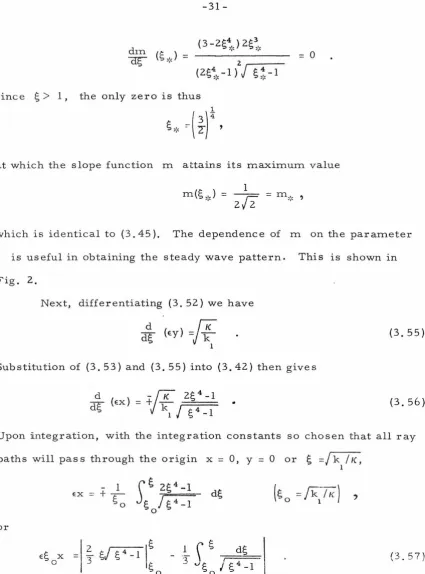
is useful in obtaining the steady wave pattern. This is shown in

Fig. 2.

Next, differentiating (3. 52) we have

d

[K

~

(ey)

=rrz-:

1

(3.55)

Substitution of (3. 53) and (3. 55) into (3. 42) then gives

d -_

{K

2g 4 -1

dS""

(ex) =

+J

~

1

j

£

4-1

(3. 56)

Upon integration, with the integration constants so chosen that all ray

paths will pass through the origin x

=

0, y

=

0 or

or

ES

x

0

i

S

s

ds

-

3

s

/

s

4 _-1

0

S

=

/k

/K,

1

'

(3. 57)

[image:36.553.70.495.53.627.2]

wave disturbance indicates only positive Ex is required. The choice

of the lower limit of integration in (3. 57) arises from the assumption of

a point disturbance at x = 0, y = 0 so that all the group lines pass

through the origin. The integral in (3. 57) ·can be readily expressed in

terms of the elliptic integrals. Thus

ES x

=I~

[s/

£

4 -1

-

s

Js

4 -1] - - 1 [F(cos-1(

~)

_!_}-

F(cos-1

(J_J

_ l

)11

,

0 3 0 0 3/z

s.,1z

s--;}J/z.

'

J

(3.58)

where F('{, "-) is the elliptic function of the first kind whose integral

representation is

1

F ('{, 1'. ) (3. 59)

=

, 0

<

b

<

µ

and 0

<

a. This function

has been studied extensively and its values for arbitrary arguments

have been tabulated (Ref. 3 ). Therefore, with the known properties of

F('{, 1'. ), (3. 58) and (3. 52) give a parametric r epresentation of the group

lines. The basic features of these two equations are shown in Fig. 3

for k

>

K and for k

=

K. In each case, Ey is linear with a positive

l 1

1

slope

r-so and inter sects the

s

-axis at

s

0

.

The behavior of EX is

more complicated. As

s

increases from unity, EX decreases from

to zero at

s

=

s

(

>

1 ). Then it increases monotonically for

s

>

s .

0 0

~(Ex)

for

s

>

1,

point

>

=

so

1

the branch of ex for

s

>

s

always lies above Ey,

0

in Fig. 3 is particularly important.

The

It

corresponds to the point source of disturbance in the physical flow field

from which all group lines originate. Therefore, it is a natural

con-sequence from the requirement of

s

>

1 that the appropriate group

lines of the wave region are given by

from

s

=

1 0

s

>

1. The limiting

0

together with the line

s

=

1 for all k

1

,

H

group line

~ 1 , thus

provide a bound for the wave region. This is shown in Fig. 4 in which

typical group lines and lines of constant

s

are plotted inside the

wave region.

The group lines are obtained from (3. 58) and (3. 52.) with k (>K)

l

being kept constant on each line. In contrast to the case of stationary

point disturbance on a uniform flow where the group lines are straight

rays from the origin, in the present case of a linear shear stream,

aside from the line y

=

0 which remains straight, all the group lines

are cubic far away from the origin. This is easily deduced from (3. 55)

and (3. 58) since for

s

large Ex ex

s

3 while EY ex

s

so that Ex ex (Eyf.

When the equation of the grc•up lines are expressed in the form

Ey

=

fn(Ex)

it can be shown that for y

>

0, they are monotonic increasing functions

extending from the origin to infinity in the fir st quadrant of the x -y

plane. For y

<

0, they decrease monotonically, terminating with zero

From (3. 58) and (3. 52), keeping s(~l) constant and varying

k (~K) we obtain the lines of constant

s.

With the exception of the

1

line

s

= 1, each

s

=

£

=

constant(> 1) has two branches. For

1

<

/

\

<

£

,

the

posit~ve

branch starts from a point on the limiting

K

cf'k:"

group line

V

-!;-,-1-

=

1 and decreases, for increasing k towards the

K 1

origin. For - >

s

,

as k increases, the negative branch which

K c 1

lies below ey = 0 decreases monotonically tending towards the asymp-tote ey = - 1 which also corresponds to

s

= 0. The negative branch of

s

= 1 has the same general behavior as the negative branches of

s

=

s

{> 1 ), however, the positive branch is missing. This curve

c

(s

=

1) warrants special attention because, though it is not a group line,

it nevertheless provides a bound for the wave region. We observe that it may be viewed as a 11_{focal curve}11 _{or "caustic" since it is an envelope} of the one parameter family of group lines. Frorn (3. 52)

k

=

K -/: 0 for

s

-

1 (3.60)

(1-ky )2.

while (3. 5 3) shows

for

s

= 1 (3.61)

Therefore, k

=

0 on

s

=

1, implying that all the wave crests are

2.

perpendicular to the x-axis there. Hence the net effect appears as if

the waves are reflected from this curve. Beyond s

=

1, it is con-jectured that edge waves, with their amplitudes decreasing exponentially, rnay exist but we shall leave this possibility for another investigation.

constant phase, inside the wave region, we may use the following

procedure:

(i)

For a given point (x , y ) in the wave region we c c

may determine the line

s

=

s

pas sing through c

it from Fig. 4.

(ii) Either from Fig. 2, or from (3. 54) we obtain

m

=

+J

s 4 -1 (Zs 4 -1 )-1

c c c

which when substituted in (3. 4 7) will give

e

.

c±

(iii) Then by using (3. 52) in (3.48) we arrive at:

k

=

±

K sec3 8

±

from which k may be deduced by evaluating

c±

the expression at

e

and

s ·

Equation (3. 46)

c± c

now gives explicitly the components of the wave

number k at (x , y ).

C± C C

(3. 62)

(3. 63)

With the knowledge that the constant phase lines are orthogonal

to k , we may graph the curves showing the traces of the wave

C±

crests. Typical traces are shown qualitatively in Fig. 5(a) for the case

of a stationary point disturbance on the surface of a linear shear flow.

The corresponding pattern for a point disturbance on the surface of a

uniform flow is reproduced in Fig. 5(b ), (Ref. 18 ) for comparison.

Apart from the shifting of the wave crests, it is immediately obvious

from Fig. 5(a) that the shear flow has the effect of suppressing the

region for a uniform flow. )

In summary, we observe that while two systems of waves, one

divergent and one transverse, exist inside the wave region produced by

a point disturbance on the surface of a linear shear flow, the traces of

the crests and the bounds to the wave region are no longer symmetric

with respect to the x-axis. In particular, the wave region boundary

approaches but never reaches the critical line ey

=

-

1 at which

U(y) = 0. The behavior of the wa·Fes near this critical line is not given

by our analysis and will be the subject of further investigation.

Final-ly, as a remark, it is quite obvious that essentially the same wave

pattern is produced by a stationary source below the surface of a

paral-lel linear shear stream.

3. A perturbation expansion

In order to make a comparison between the present geometric

optics method and the integral transform method, which will be dis

-cussed in Chapter IV, we shall consider here a perturbation expansion

in terms of a small

U

(y ),;, .

l

By regarding

iu

(y)

I

«

1,

l we are actually

limiting the region of validity of the resulting solution to

IY

I

«

1

E in

view of the definition of

U

(y), (3. 51 ), For a small shear gradient

l

(i.e. E small) this may still represent an appreciably large region

in the physical space.

:::::

By expanding (3.49) in powers of

U

(y), we have

l

k z

k

l

(3. 64)

whereas the reciprocal of (3. 64) is

{]

kz k4 kl.

l

2 _l_

+

u{is~

-r

(:~~

-

i1·

k

(± 1) Kz.

l _O(U3

)

~

k

-;

_k2.

-

u,(k:-)

. l

J

2.

_l_ - 1 _{- -1}

Kl Kz

(3. 65)

By substituting (3.64) and (3.65) in (3.42), we obtain

dx - <::!±

dy

kz kz.

3

_l_

6

_1_

(:: K:r'

t

/(

;K~l)

+

O(u: ) } , (3. 66)

in which the

+

or - sign is taken according as y is

>

or

<

0.

Using the known result that k and K are constant on each group

line and

u

(y)

l =

ey,

±~I

k: I

x

-

_y

""

-!

)

\Kl.

we obtain by simple integration

ITT

k'[

1

t2

t

Ey - 1

-l';'

-Ir"+

f_:

Kl.

K2

I

K2

I

(:~

-r

'

kl.

2 _1_

Kl ₄

- 3

2

l

-1

(3.67)

which is the required expansion of the group lines. In (3. 67), the

integration constant has been chosen for a point disturbance located at

x

=

0, y = 0, so that all the group lines pass through the origin of the

x-y plane. Plotting of the group lines from (3. 67) is straightforward.

However, as the group lines over a m uch larger region have already

been traced in Fig. 4, we will not repeat this operation.

We proceed to determine the boundary of wave region and the

loci of constant phases (such as the wave crests) within the wave

r egion. The extent of the wave region can be deduced from Eq. (3. 67)

for the ray traces. To simplify writing, we introduce the parameter

so that (3. 67) becomes

1

13

=

(kl

I

K2 - 1 )2

5 6)

-

+ -

+

O(eyf,

133

135

(3. 69)

where

M

=

x/

IYI

(3. 70)

which may be regarded as a function of

(13;

ey), possessing the

expan-sion for (ey) small. Along each ray track, _{k '}

l

and hence 13 remain

constant. It therefore follows that at the bounding ray track, which

envelopes the wave field, one must have (oM/ 813) = 0, the differentia-tion being for fixed y. Now, by (3. 69),

(

~ ~)

y =

l

2

-13

\ )

+

E y

l

2 - 13

\

+ :

J

+ } (

E y )

2 ( 2

-13

~

-

~ ~

- :

~

) = Q •

(3.71)

The solution of (3. 71), say 13=13,:,(ey), is obtained to have the expan

-sion

(3. 72)

as can readily be verified. It may be remarked here that only the

positive branch of 13 ,:, is chosen since M, as defined by (3. 70), is

non-negative. Substituting 13 ,:, of (3. 72) for 13 in (3. 69), we obtain after some regrouping, the following result for the boundary of the

wave field,

(3. 73)

final result of x,:,(y); hence the boundary of wave region is symmetric

with respect to the x -axis up to O(ey)2• It is further noted that the

stationary waves exist in the region x:

>

x,:,(Y ), that is, on the down-stream side of x = x_._(

.,.

y). Although the envelope of the wave field is

symmetric in y, the detailed wave pattern is generally not

sym-metric with respect to the body trajectory y = O. Since, as indicated

by (3. 69),

f3 ,

and hence k ,

1

are neither even or odd in y. In fact,

the value of k (x ... (y), y), which is the x-component of the wave

num-1 -~

ber at the boundary of the wave field, is different for different signs l

of y, as can be seen from k {x ... , y)

=

K ( 1

+[3

z.

.

.J2

-1 ~ ~ and (3. 72). This also

implies that x = x,:,(y) and x = x,:,(-y) are no longer ray tracks.

The above result may be expressed alternately in terms of

cylindrical polar coordinates (r, a) defined by

x = r cos

a

y = r sina (3.74)

so that at the boundary x = x,:,(y), the value of <J = a,:,(r;e) may be

expanded as

a

...

(

r ; e ) =

a

(

r )

+

e r

a (

r )

+

(er )z.

a (

r )

+

0 (er )3

.,. 0 1 z. (3. 75)

Upon substitution of (3. 74) and (3, 75) in (3. 73), together with

neces-sary expansions,

a

o' a

1, CYz. are readily determined; the final result

is

-1 1

-

1{

_{1 )} O" ₌ tan _- = sin

3

O" = 0 0

2/ 2 1

(J ₌

-

3Jz

_sin4 _{<J =}

-

12

~

2 0 (3. 76)

in which the

+

or

=±(sin-

1

(1/3)-

~

(er)'+O(<r)1

(3. 77)

sign is for y

>

or

<

0. This result shows that

the over -all effect of the uniform shear is suppressing the wave field

to a smaller region than in the uniform flow case, the deviation being

of second order for (er) small, These salient features are shown in

Fig.

6

.

The contours of constant phases (such as the wave crests) can

be calculated as follows. We note first that the slope of a constant

phase line,

cp

=

canst. , at the free surface is given by

acfl

I ax

04>

I

ay

k

l

=

-

k

2.

(3. 78)

by virtue of the characteristic equations, or more directly by the

definition of the phase function. The term k /k on the right hand

1

z

side of (3. 78) can be regarded as a known function of x and y in

view of (3, 68), (3.69) and (3.64). Consequently, the above first order

differential equation can, in principle, be integrated. However, the

actual calculation may prove formidable. In view of the complicated

nature of the functions k (x, y), k (x, y), it is best to seek a parametric

1 2.

integration. It turns out that a convenient parameter is @, defined by

k

/K

=

sec®

1

Then (3. 69) becomes

or

1

13

=

(kz.

/Kz

-

1 )2

=

tan@ 1

(3. 80)

with

p(®) = 2 tan® + cot® q(@)

=

p(® ) - cot3®

By making use of the expansion (3. 65 ), (3. 78) can be expressed in

terms of ® as

(

~)

=

(sgn y )

I

:

2 \

=

(sgn y)tan® {l + 2e.y cscz.® +e.z.y2 csc2(8:,(1-2 cot2

®

)}.

Y

4>=

c

i

(3. 81)

We assume that the integral of (3. 81) may be expressed in the following

form

2

y

=

!

.

e.nyn(® ) + O(e.3) (3. 82)

n=o n=o

The two sets of functions {x (®)} and {y (® )} are not linearly

in-n n

dependent since they are related by (3. 80). In fact, upon substitution

of (3. 82) in (3. 80), we find that for y

>

0,

x

=

y p

+

yz q

+

Yo3 s

l 2 l (3. 83)

whereas for y

<

0 the signs of all the terms on the right hand sides of

(3. 83) are changed. Furthermore, substituting (3. 82) in (3. 81) yields

x = ±

y

tan®

0 0

.;._ =±

[y

+ 2y

y

csc2®)tan®,

l l 0 0

(3.84)

x =±

{y

+2y

y

csc2®+

y

[2y +y~l-2cot2®)]csc2®}tan®

2 2 0 1 0 l 0

where ;;.

0 denotes dx0 (®)/d®, etc, and the + or sign is for

y

>

or

<

0 respectively. Differentiating the first equation of (3. 83),

we have

(2tan® + cot®)y + (2sec2® - csc2®)y

0 0

After x is eliminated by making use of (3, 84) we obtain the equation

0

for y as

0

which has the integral

(cot® - 2 tan®}y

0

y =A sin®cos2®

0 0

where A is an arbitrary constant of integration.

0

(3,85)

(3.86)

Similarly, from the second equation of (3. 83) and (3, 84) we

derive the differential equation for y

1

as

d ( yl ) •

d\85

=

2A y

sin®cos2® 0 0

(3. 87)

This equation can be integrated explicitly, giving

y = A sin®cos2

®

+A 2 cos4®cos 2®

A being another arbitrary constant. Integration of higher order

equations becomes increasingly tedious; the integral of y will not be 2.

given here.

Summarizing, we have determined the lines of constant phase

in the parametric forrn

x =A {cos@(l+sin?..@) + 2eA sin@cos5@+ O(eA )2.}

0 0 0

y =: A {sin@cosz.@ + eA cos4@ cos 2@ + O(eA )2}

0 0 0

(3.89)

(3. 90)

in which the constant A

1 has been absorbed into the higher order

terms. The constant A can be related to the phase i/> by noting that

0

the phase function

cp ;:;

xk

+

y k

=

A K { 1

+

0 (EA } }

l z 0 0 (3.91)

where in the last step use has been made of (3. 89), (3. 90) for x(@)

and y(@), and of (3. 81) for (k /k ),

2 l (3. 79) for k . l

Hence

(3. 92)

and from a wave crest to another,

cp

changes by 2mr(n=l, 2, . . . ).

The leading terms of x(@) and y(@) are the well-known Kelvin

ship wave pattern in a uniform stream. There are two wave systems

within the region largtan(y/x)j

<

sin-1(1/3), one corresponding to the

range 0 <@<@

~:::: ' (@ .. _

=

tan

-1

13

.

.

.

=

tan-1(/2./2)) and the other to

.. ,.. .., ..

®,

:

,<

@<

TT/

2, called respectively the diverging and transverse waves.

In the present case of a uniform shear, the position and wavelength of

these waves are shifted by an amount of order e. From (3. 90) it is

noted that \k \ increases for y

>

0 (in which region k

<

0) and

decreases for y

<

0 (where k

>

0) with increasing shear gradient

2.

E, Thus the resulting configurations of constant phase lines are not

symmetric with respect to the x -axis; these qualitative features are

shown in Fig. 6. The perturbation expansion studied in this section

shows that the resulting steady wave pattern due to a point disturbance

on the surface of a linear parallel shear flow in the region y

«

1 / e

has essentially the same basic features as the solution of the previous

section. Thus, it constitutes a good approximation. The results

obtained here will be compared with that obtained by the method of

IV. INTEGRAL TRANSFORM METHOD

A combination of Fourier transform and Laplace transform

has been used by several writers (see DePrima and Wu (Ref. 2 ) and

Wu and Mei (Ref. 21) ) in dealing with problems of steady and unsteady

surface waves. A slight extension of the cla