Volume 2008, Article ID 480835,13pages doi:10.1155/2008/480835
Research Article
About Noneigenvector Source Localization Methods
S. Bourennane, C. Fossati, and J. Marot
Ecole Centrale Marseille, Institut Fresnel, UMR 6133 CNRS, Universit´es Aix Marseille, Campus de Saint J´erˆome, 13397 Marseille Cedex 20, France
Correspondence should be addressed to S. Bourennane,[email protected]
Received 23 August 2007; Revised 30 January 2008; Accepted 21 April 2008
Recommended by Fulvio Gini
Previous studies dedicated to source localization are based on the spectral matrix algebraic properties. In particular, two noneigenvector methods, namely, propagator and Ermolaev and Gershman (EG) algorithms, exhibit a low computational load. Both methods are based on spectral matrix structure. The first method is based on the spectral matrix partitioning. The second one obtains directly an approximation of noise subspace using an adjustable power parameter of the spectral matrix and choosing a threshold value. It has been shown that these algorithms are efficient in nonnoisy or high signal to noise ratio (SNR) environments. However, both algorithms will be improved. Firstly, propagator is not robust to noise. Secondly, EG algorithm that requires the knowledge of a threshold value between largest and smallest eigenvalues, which are not available as eigendecomposition, is not performed. In this paper, we aim firstly at demonstrating the usefulness of QR and LU factorizations of the spectral matrix for these methods and secondly we propose a new way to reduce the computational load of a high resolution algorithm by estimating only the needed eigenvectors. For this, we adapt fixed-point algorithm to compute only the leading eigenvectors. We evaluate the performance of the proposed methods by a comparative study.
Copyright © 2008 S. Bourennane et al. This is an open access article distributed under the Creative Commons Attribution License, which permits unrestricted use, distribution, and reproduction in any medium, provided the original work is properly cited.
1. INTRODUCTION
The most popular high-resolution method for source local-isation ismultiple signal classification(MUSIC) [1,2]. The principles of this method are to exploit the structure of the vector space which is spanned by the measures collected upon the sensors. This vector space is the direct sum of the signal subspace and the noise subspace, which are orthogo-nal. In the MUSIC method, the orthogonality between signal and noise subspaces is exploited. Source localization is based on the structure of the spectral matrix of the sensor outputs, that is, the Fourier domain version of the covariance matrix of the received signals. To cope with a spatially correlated additive noise, the appropriate “cumulant matrix” of the sig-nals [3,4] is used instead of spectral matrix. In practice, the main limitation for real-time implementation of the high-resolution methods is the computational load. In the last two decades, several algorithms without eigendecomposition have been proposed [5–8]. In [5], propagator method is developed. It is based upon spectral matrix partitioning. In [6,7], fast algorithms for estimating the noise subspace projection matrix are proposed. These algorithms require a
prior knowledge of threshold value and an adjustable power parameter. The problem of the choice of threshold value is not completely solved. Independently, Bischof and Shroff [8], and Strobach [9] developed two other noneigenvector algorithms for source localization based on QR factorization. All these algorithms [5–9] assume that the number of sources is known. The existing criteria [10–13] cannot be applied because the noneigenvector algorithms do not calculate the eigenvalues of the spectral matrix.
In this paper, we propose new versions of the prop-agator and EG localization methods [5,7] which employ a factorized spectral matrix and which are efficient in noisy situations. To this end, we use the upper triangular matrices obtained by the LU or QR factorizations of the spectral matrix. We also propose a noneigenvector version of MUSIC algorithm, where singular value decomposition (SVD) is replaced by a faster algorithm to compute leading eigenvectors.
meant to concentrate all the signal information in the upper-left corner block matrix of the upper triangular matrix.
We recall that the LU factorization [14, 15] consists in decomposing the spectral matrix Γ as Γ = LU where
L is a unity lower triangular matrix (“unity” meaning that LLH = I, where superscript (·)H
represents the Hermitian transposition of (·)) andUis an upper triangular matrix (UTM). QR factorization consists in decomposing the spectral matrix Γ as Γ = QR where Q is a unitary matrix and R is UTM [14, 15]. In both factorizations, it has been shown that the diagonal elements of R or
U matrices tend to the eigenvalues of the spectral matrix in decreasing order [14, 15]. We propose to use these elements to estimate the number of sources and to determine the threshold value needed in Ermolaev and Gershman algorithm [7]. We also exploit the benefit of the factorization algorithm regarding the new rearrangement of the elements of the spectral matrix in the resulting upper triangular matrices R or U. All the signal information is focused in the upper-left corner block matrix of size equal to the number of sources. This block matrix contains the largest diagonal elements of the factorized matrix. In other words, it concentrates the signal information which is scattered in all spectral matrix elements. This concentration improves the propagator operator. Indeed, according to the partitioning procedure defined in the propagator method [5], when we use R or U, the estimation of the propagator uses this block matrix. This is in accordance with the principle of the propagator theory, and the obtained result is similar to that obtained in the nonnoisy case. This new way leads to minimize the influence of model errors. This permits the propagator method to estimate accurately the directions-of-arrival of the sources in the presence of noise.
We also propose a new solution to accelerate the subspace-based high-resolution method. A fixed-point algo-rithm is adapted to compute the leading eigenvectors from the spectral matrix.
The remainder of the paper is organized as follows: problem statement is presented inSection 2. InSection 3, we give an overview of the propagator localization method and the outline of Ermolaev and Gershman algorithm.Section 4
details improved versions of propagator and EG methods. In particular it describes the propagator estimation using LU or QR factorization. It also details the estimation of the threshold value for the EG method. It presents how a statistical criterion can be adapted to the estimation of the number of sources. It provides a solution to accelerate the subspace-based high-resolution MUSIC method, using fixed-point algorithm. Section 5 provides a study about performance analysis of the reviewed methods. Section 6
provides the numerical complexity of the reviewed and pro-posed algorithms. Comparative results are given inSection 7
on simulated data. Last section concludes the paper.
2. PROBLEM STATEMENT
Consider an array of N sensors receiving the wave field generated byP (P < N) narrow-band sources in the presence of an additive noise. The received signal vector is sampled
and the FFT algorithm is used to transform the data into the frequency domain, we present these samples by [1,2,5]
x(f)=A(f)s(f) +n(f). (1)
In the rest of the paper the frequency f is omitted. In (1)xis the Fourier transform of the array output vector,
s=s1,. . .,sP
T
(2)
is the signal source vector, and
n=n1,. . .,nN
T
(3)
is the additive noise vector. The (N×P) matrix
A=a(θ1),. . .,a(θP)
(4)
is the transfer matrix of the sources-sensors array system with respect to a chosen reference point. The steering vectors
a(θi), where θi, i = 1,. . .,P, is the DOA of the ith source measured with respect to the normal of the array. For a linear uniform array withNsensors the steering vector is
a(θi)=√1 N
1,e−jϕi,e−2jϕi,. . .,e−(N−1)jϕiT, (5)
where ϕi = 2π f(d/c) sin(θi), dis the sensor spacing, and cis the wave propagation velocity. Assume that the signals and the additive noises are stationary and ergodic zero-mean complex-valued random processes. In addition, the noises are assumed to be uncorrelated between sensors, and to have identical variance σ2 in each sensor. It follows from these
assumptions that the spatial (N×N) spectral matrix of the observation vector is given by
Γ=AΓsAH+Γn, (6)
where
Γ=ExxH,
Γs=EssH,
Γn=EnnH=σ2I,
(7)
whereE[·] denotes the expectation operator andIis the (N×
N) identity matrix.
In the following, the propagator and EG algorithms are presented and improved.
3. OVERVIEW OF EXISTING NONEIGENVECTOR METHODS
We present in this section two noneigenvector methods, propagator and “Ermolaev and Gershman” methods.
3.1. Propagator method
3.1.1. Principles of propagator method
first rows are linearly independent, there exists aP×(N−P) matrixΠΓcalled propagator operator, such that [5]
A=ΠHΓ A, (8)
whereAandAare theP×Pand (N−P)×Pblock matrices, respectively, obtained by partitioning the transfer matrixA:
A=AT ATT. (9) Define theN×(N−P) matrixDΓ:
DΓ=
ΠTΓ −IN−P
T
, (10)
whereIN−Pis the (N−P)×(N−P) identity matrix. Now, using (8) and (9), we have
DHΓA=ΠHΓ A−A=0. (11) In other words, the (N−P) columns ofDΓare orthogonal to the columns ofA. This means that the subspace spanned by the columns of the matrixDΓ is the same as the subspace spanned by the noise subspace given by the eigenvectors associated with the (N−P) smallest eigenvalues of matrixΓ. We then obtain the DOAs of the sources by the peak positions in the so-called spatial spectrum [5,14]:
FPr(θ)=
a(θ)H DΓ DHΓ a(θ)
−1
. (12)
Equation (12) shows that the propagator algorithm is based on the noise subspace spanned by the columns of matrixDΓ. The computation of matrixDΓrequires a prior knowledge of the sources DOAs ((8) and (10)). In practice, these DOAs are unknown. However, the matrixDΓ must be estimated only from the received data [5,17].
3.1.2. Estimation of the propagator from the received signals
We define the data matrix X containing all K signal realizations asX=[x1,. . .,xK].
MatrixXis partitioned (in the same way as in (9)) asX=
[XT XT]T. The resulting spectral matrix will be expressed as follows [18]:
Γ=
Γ11+σ2Ip Γ11ΠΓ
ΠHΓΓ11 ΠHΓΓ11ΠΓ+σ2IN−p
=
G11 Γ12
Γ21 G22
,
(13)
whereΓ11andΓ12are, respectively, (P×P) and (P×(N−P))
matrices, using the partition of matrixA((8) and (9)), we haveΓ11=AΓsA
H .
In nonnoisy environment (σ2 =0) in [18], the relation
Γ12=Γ11ΠΓis used to estimateΠΓ:
ΠΓ=Γ−111Γ12. (14)
In the presence of noise, (14) is no longer valid. An estimation of the matrixΠΓ is provided by minimizing the
cost function J(ΠΓ) = Γ12 −G11ΠΓ2, where ·is the Frobenius norm. The optimal solution is given by
ΠΓ=G−111Γ12. (15)
In practice, the data are generally impaired and the SNR value is not always high. Then, the performance of propaga-tor method depends on the signal information contained in the block matrixG11with respect to the noise and its linear dependency with the block matrixΓ12. In [16], a statistical
performance study concerning the propagator method is presented.
3.2. Ermolaev and Gershman method
The conventional high-resolution algorithms are based on the noise subspace spanned by the eigenvectors associated with the smallest eigenvalues of spectral matrix. In order to reduce the computational load, several methods have been proposed for estimating the noise subspace without singular value decomposition (SVD). In [6,7], the proposed algorithms are based on the properties of the spectral matrix eigenvalues. A threshold value and an adjustable parameter are used in order to make an approximation of noise subspace projection matrix.
The Ermolaev and Gershman algorithm relies on the eigenvectors of the spectral matrix:
Γ=
P
i=1
λiPi+ N
i=P+1
λiPi=VsΛsVsH+VnΛnVHn, (16)
whereλi, i = 1,. . .,N, is theith eigenvalue ofΓandPi =
vivHi is the associatedith eigenprojection operatorVi, being theith eigenvector. The well-known properties are [1,2] as follows.
(i) The smallest eigenvalues of Γ are equal toσ2 with
multiplicity (N−P). Then, we have
λ1≥ · · · ≥λP> λP+1=λP+2= · · · =λN=σ2, (17)
(ii) The eigenvectors associated with the smallest eigen-values are orthogonal to the columns of matrixA. Namely, they are orthogonal to the signal steering vectors:
Vn=
vn+1,vn+2,. . .,vN ⊥
aθ1
,aθ2
,. . .,aθP , (18)
where the columns of the (N ×(N −P)) matrix Vn are the (N − P) eigenvectors associated with the (N − P) smallest eigenvalues of the spectral matrix. The columns of matrix span Vnthe noise subspace [2]. This orthogonality is used for estimating the DOAs. Vs = [v1,v2,. . .,vP] is called the signal subspace,Λs = diagλ1,. . .,λPandΛn = diagλP+1,. . .,λN. For any integer valuem, the calculation of the estimate of the noise subspace projection matrix can be found in details in [7]; we have
VenVHen=mlim→∞
1 λs
Γ
m +I
−1
where the threshold valueλsis bounded byλPandλP+1:
λP> λS> λP+1. (20)
In (19), index “en” in Ven refers to Ermolaev and Gershman. Equation (19) shows also that the estimation of the noise subspace projection matrix depends on the threshold value λs which separates the largest and the smallest eigenvalues of the spectral matrix. In practice, the determination of this value still remains very difficult. In [6], the inverse power algorithm is used to calculate the threshold value, which is taken equal to the smallest eigenvalue of the spectral matrix. However, the stability of this algorithm is not always ensured. More precisely, the matrix inversibility is not ensured.
Propagator method is not robust to noise, and Ermolaev and Gershman method requires the threshold value. In the next section, we propose to solve both problems by introducing LU and QR factorization methods.
4. PROPOSED IMPROVEMENTS FOR NONEIGENVECTOR METHODS
In this section, we show how LU or QR factorization of the spectral matrix can improve propagator and EG algorithms. We propose a method for the estimation of the number of sources and an accelerated version of MUSIC algorithm.
4.1. Propagator method using upper triangular matrices
In this subsection, we insert an LU decomposition step in propagator method to improve the robustness to noise of propagator method. The properties of the upper triangular matrix are used to minimize the influence of model errors.
Assume that spectral matrixΓ bears LU factorization, then it is expressed as [19,20]
Γ=LU=
L11 0 L21 IN−P
U11 U12 0 U22
; (21)
we have
Γ=
L11U11 L11U12 L21U11 L21U12+U22
. (22)
Using (13), (14), and (22), we have
L11U12=L11U11ΠU. (23)
Finally, the novel estimate of the propagator operator using LU factorization is
ΠU =U−1
11U12. (24)
If we calculate the following product,
U11 U12 0 U22
U−111U12 −I
=
0 −U22
. (25)
We show that the columns of matrixU−111U12 −I
form a basis for the eigenvectors associated with the smallest eigenvalues and the block matrixU22contains the smallest eigenvalues of matrixΓ. This result confirms that the propagator (see (15)) estimated from the LU factorized spectral matrix (24) is in accordance with the propagator principle.
As mentioned in several papers [12,19,21], (25) shows that the smallest eigenvalues are in the lower-right corner of U, that is, the block matrix U22. The useful signal components are concentrated in matricesU11andU12. This yields a better robustness to noise compared to the case, where the classical propagator method is applied.
Following similar calculations with the QR factorization, we obtain
ΠR=R−1
11R12. (26)
In the same way as for LU-based method, we have
R11 R12 0 R22
R−1 11R12
−I
=
0 −R22
. (27)
As in the LU factorization the smallest eigenvalues are in the lower-right corner of R, that is, the block matrixR22. The
columns of matrix R−111R12 −I
form a basis for the eigenvectors associated with the smallest eigenvalues and the block matrix
R22contains the smallest eigenvalues of matrixΓ. Let the matrices
DU=
ΠTU −IT,
DR=
ΠTR −I
T .
(28)
It follows that the DOAs of the sources are given by the positions of the maxima of the following functions:
FU−Pr(θ)=
aH(θ)DUDHUa(θ)
−1
,
FR−Pr(θ)=
aH(θ)DRDHRa(θ)
−1
.
(29)
Column vectors ofDU andDRdo not form an orthonormal basis, as was provided by SVD method. However, in general, this is not necessary since the roots ofFU−Pr(θ) orFR−Pr(θ)
are, respectively, identical for all basisDU orDRof the noise subspace [8].
Both LU and QR factorization procedures rearrange the elements of the spectral matrix by concentrating all the signal information in the upper-left corner block matrix of the upper triangular matrix, whereas signal information is scattered arbitrarily in the initial matrix. Indeed, this block matrix contains the largest elements of the factorized matrix. This permits the propagator method to keep its good performance even in the presence of noise.
4.2. Improvement of EG method: threshold value estimation using triangular factorization of spectral matrix
the EG algorithm [7]. We propose an analytical solution based on the linear algebra results developed in [19] and recently improved in [20] concerning the eigenvalues of the symmetric and definite positive matrices.
Let us consider that the spectral matrixΓhas a numerical LU factorization, then its factorization is [19,20]
Γ=LU=
L11 0 L21 IN−P
U11 U12 0 U22
. (30)
Following the algebra results published in [19,20], we have
λP≥λmin
L11U11
U22λP+1, (31)
where L11 is a (P×P) unit lower triangular block matrix,
U11is (P×P) upper triangular block matrix, L21 ,U12, and
U22are the (N−P)×P, P×(N−P) and (N−P)×(N−P) block matrices, respectively. λmin
L11U11 is the minimal eigenvalue of the (P×P) matrixL11U11. Several papers [19–
22] were dedicated to the question of whether there is a strategy that will force entries with magnitudes comparable to those of eigenvalues to concentrate them in the lower-right corner of U, so that LU factorization reveals the numerical rank.
The QR factorization of the spectral matrix is [19,20]
Γ=QR=Q
R11 R12 0 R22
, (32)
whereR is an (N×N) UTM andQ is a (N×N) matrix with orthonormal columns.R11,R12, and R22 are the (P×
P), P×(N −P), and (N−P)×(N−P) block matrices, respectively. Besides being able to reveal rank deficiency of Γ, a QR factorization with a small R22 block is very useful
in many applications, such as in rank deficient least squares computation [22]. Following [20] we have the minimal eigenvalue ofR11, denoted byλmin
R11
, and the maximal eigenvalue ofR22, denoted byλmax
R22
=R22, bounded
[19,20,22] by
λP≥λmin
R11
R22λP+1. (33)
The EG algorithm [7] requires the prior knowledge of the last signal eigenvalue and the first noise eigenvalue to estimate the threshold. In this paper, we propose to improve the traditional EG algorithm concerning crucial threshold value estimation problem. According to the previous expressions (25), (27), (31), and (33) the valuesU22orR22can be chosen as threshold valueλs.
The spatial spectrum corresponding to EG algorithm for source localization becomes
F(θ)= lim
m→∞
aH(θ)
1 λS Γ
m +I
−1 a(θ)
−1
. (34)
withλS=λUS =U22orλS=λRS =R22.
We have concluded from numerous simulations that values close to 10 are convenient. Close values were experi-mentally shown, in [6,7,23], to be the appropriate ones.
4.3. Estimation of the number of sources using the upper triangular matrices
In this subsection we show how to estimate the number of sources. We use the diagonal elements, which are in decreasing order, of the matrices R orUfor this purpose. We propose to add this step in the noneigenvector source localization procedures, which currently suffer with this problem in real-world applications. Indeed, in propagator method, we need the number of sources to partition matrices
Γ, R,orU.
The estimation of the numberP of sources is a delicate problem. Several methods have been developed. The two most popular methods are akaike information criterion (AIC) [10] and minimum description length (MDL) [11]. These algorithms are based on spectral matrix eigenvalues. This is the main difficulty, while applying the noneigenvector methods, as the eigenvalues are supposed to be known. In this paper, we propose to use the diagonal elements of the UTM obtained thanks to the triangular factorizations of the spectral matrix for estimating the number of sources. Indeed, asymptotically the diagonal elements of RorUmatrix tend to the eigenvalues ofΓ.
Algorithms for LU factorization based on Gaussian transformations are given, for example, in [15, Section 3.2] or in [24]. Algorithms for QR factorization based on Householder and Givens orthogonalization procedures are described in [15, Sections 5.2 and 5.3] and in [25]. In this paper, we refer to the Householder orthogonalization procedure, which is generally preferred to Givens method because it is twice fast.
The estimation of the number of sources is usually based on the application of AIC or MDL criteria to the eigenvalues of the spectral matrix. We propose to use the diagonal elements of the matrixUorRinstead of eigenvalues, as these elements tend to the eigenvalues [14,15]. According to [23], another simple way to estimate the number of sources is based on the successive comparison of diagonal elements of the matrixUorRdefined as
Λu=diag
u1
uN ,u2
uN ,. . .,uN
uN
(35)
or
ΛR=diag
r1
rN , r2
rN ,. . .,rN
rN
, (36)
whereuiandrifori=1,. . .,Nare the diagonal elements of
UandRin decreasing order, respectively.
For instance, we haveu1≥u2≥ · · · ≥uNandr1≥r2≥ · · · ≥rN.
It is easy to see that lim t→∞Λ
−1
U =tlim→∞Λ−R1 = diag[0, 0,. . ., 1, 1]. Then, the number of zeros in this diagonal matrix gives the number of sources. Choosing a too small value oftdoes not permit to distinguish clearly between null and 1 values, choosing a too high value oftincreases the computational load.
4.4. MUSIC without eigendecomposition
In this subsection, we present an overview of the traditional multiple signal characterization (MUSIC) method and pro-pose a noneigenvector version of MUSIC.
4.4.1. Principles of MUSIC method
MUSIC method provides the DOAs of the sources by the peak positions in the so-called spatial spectrum [5,14]:
Fmusic(θ)=
aH(θ)VnVHna(θ)
−1
. (37)
The maximum values ofFmusic (θ) yield the source DOAs.
MUSIC requires the eigenvectors of the spectral matrix that span the noise subspace. Traditionally, singular value decomposition (SVD) of the spectral matrix is performed. We propose to replace singular value decomposition by fixed-point algorithm [26] and thereby accelerate MUSIC algorithm.
4.4.2. Acceleration of MUSIC algorithm with fixed-point algorithm
We present the fixed-point algorithm for computing leading eigenvectors and show how it can be inserted in MUSIC to compute the noise subspace.
Fixed-point algorithm for computing thePorthonormal basis vectors is summarized in the seven following steps.
(1) Choose P, the number of eigenvectors to be esti-mated. Consider spectral matrixΓand setp←1. (2) Initialize eigenvectorvp of sizeN×1, for example,
randomly.
(3) Updatevpasvp←Γvp.
(4) Do the Gram-Schmidt orthogonalization process
vp←vp−
p−1
j=1(vTPvj)vj.
(5) Normalizevp by dividing it by its norm:vp ← vp/ vp.
(6) Ifvphas not converged, go back to step (3).
(7) Increment counterp←p+ 1 and go to step (2) until pequalsP.
The eigenvector with dominant eigenvalue will be measured first. Similarly, all remainingP−1 basis vectors (orthonormal to the previously measured basis vectors) will be measured one by one in a reducing order of dominance. The previously measured (p −1)th basis vectors will be utilized to find thepth basis vector. The algorithm for pth basis vector will converge when the new valuev+
p and old valuevP are such that vT
pv+P = 1. It is usually economical to use a finite tolerance error to satisfy the convergence criterion|vPTvP+ − 1| < δ, whereδ is a prior fixed threshold and |·| is the absolute value. LetVs=[v1,v2,. . .,vP] be the matrix whose columns are thePorthonormal basis vectors. Then,Vsis the subspace spanned by theP eigenvectors associated with the largest eigenvalues. It is also called ”signal subspace.” The projector onto the noise subspace spanned by the (N−P)
eigenvectors associated with the (N−P) smallest eigenvalues isI −VsVHs =Vf nVHf n. This estimated projector can be used in (37). InVf nandVHf n, index “f n” refers to fixed point.
5. PERFORMANCE ANALYSIS OF THE CONSIDERED ALGORITHMS
In this section, we investigate the performance of the considered methods in terms of mean-squared error of the source bearing estimates. This investigation is inspired by previous results in [27–29].
A common model for the null spectrum function associated with the propagator, EG algorithm as well as with MUSIC is
M(θ)= aH(θ)Ba(θ) , (38)
where B = D DH with D = DΓ, D
U, orDR or B =
VnVHn,B=Vf nVHf n, orB = VenVHen
The DOAs are the arguments of the minima ofM(θ), when no perturbation affects matrixB. When noise is present in the data, or when there are some uncertainties on the data model, the function from which we search for the minima in order to determine the DOA estimates is
M(θ)= aH(θ)Ba (θ) (39)
with a first-order expansion of the first derivativeM(θ) of
M (θ) around the bearing estimates θp and with a first-order expansionB=B+ΔBit has been shown in [28] that the error on the bearing estimates,Δθp=θp−θp, is given by
Δθp= −
RealaHθ p
ΔBgθp
gHθ p
Bgθp
, (40)
where g(θ) is the vector whose components are the first derivative of the components of a(θ). In order to compute the DOA estimation error (40), it is necessary to evaluate matrixΔBwhen the data matrix is perturbed byX= Xf + ΔX, where X = [x1,. . .,xK] with K number of snapshots of measurement vectors x andXf is the data matrix with no perturbation and whereΔXis the additive perturbation matrix. From the partition (9), we can writeXf =[XTf XTf]
T . Following the calculation given in [27,28], in the case of the MUSIC method using SVD, that is,B = VnVHn, the authors of [28] have shown that
Δθp= −
RealaHθ p
T1ΔXHBgθ p
gHθ p
Bgθp
(41)
withT1 = VsΛ−s1VHs,Vs = [v1,. . .,vP], Λs = diag[λ1,. . .,
λP] which gives the error on the bearing estimates for the EG and fixed point, by replacingBby VenVHenand Vf nVHf n, respectively.
Following the same calculations [27,28], we obtain for the propagator method
Δθp= −
RealaHθ p
T2ΔXHDDHgθ p
gHθ p
DDHgθ p
withD=DΓ, DU, orDR
T2= −
(XfX H f )−1·Xf
0
. (43)
In [28, 29], the MSE, that is, E[|Δθp|2] has been derived from (41) for an additive perturbation matrixΔXwith zero-mean uncorrelated random components with equal variance σ2(see [28,29]), for the MUSIC method, we have
EΔθp2
=σ2aH
θp
T1TH1a
θp
2gHθ p
Bgθp
(44)
withB = VenVHen.
When EG method is considered B = VenVHen, and when MUSIC with fixed-point algorithm is considered,B =
Vf nVHf n.
We easily deduce that the MSE expressions are
EΔθp2
=σ2
gHθ p
DDHDDHgθ
p
aHθ p
T2TH2a
θp
2gHθ p
DDHgθ
p
2
(45)
withD=DΓ, DU, orDR.
We therefore provided the expressions of the error ((41) and (42)) and variance ((44) and (45)) for the DOA estimation by the considered methods.
6. ALGORITHM COMPLEXITIES
In this version, we provide the theoretical expressions of the numerical complexities of the proposed noneigenvector methods.
6.1. Propagator and Ermolaev and Gershman methods
The main advantage of the methods presented in this paper, namely, propagator (29) and Ermolaev and Gershman methods (34) is their low computational load. Indeed, these methods do not require the costly eigendecomposition of the spectral matrix. The complexity of the LU factorization algorithm is [19,25]NLU
op(N)≈N3/3. The number of
opera-tions required by Householder QR factorization algorithm [25] isNopQR(N) ≈ 2N3/3. The number of multiplications
involved in calculating an upper triangular matrix inversion is N2. Proposed EG method requires consequently around
N3/3 +N2operations. It is well known that the number of
operations to calculate an (N ×N) matrix Γ inversion is N3, so the original EG method needs aroundN3operations.
Considering the number of sensors which is usually used, the proposed method is faster than the traditional one.
Following [16] the cost involved by the estimation of the propagator from the spectral matrix of the received signals (15) isN2P+P2N+P3. The computational load involved
by the LU or QR-based methods to obtain ΠU (24) orΠR (26) is P2(N −P + 1). The proposed methods are based
on the LU or QR factorization which requires considerably less computations than eigendecomposition. This result is interesting for large arrays with few sources which is often the case in underwater acoustics.
6.2. MUSIC algorithm and accelerated version
The traditional MUSIC method estimates the noise sub-space eigenvectors by singular value decomposition (SVD). Then, we compare the computational complexities of the traditional MUSIC method and the proposed accelerated version of MUSIC method through the comparison of the computational complexities of SVD and fixed-point algorithm.
One well-known SVD method is the cyclic Jacobi’s method. The Jacobi’s method which diagonalizes an (N ×
N) symmetric matrix requires around N3 computations.
The computational complexity of fixed-point algorithm is computed as follows. LetItbe the number of iterations used in converging the algorithm to obtainvp. Then, the estimated computational complexity is given in the following steps.
(i) The Gram-Schmidt orthogonalization for vp (any value ofp) implies aroundNPItoperations.
(ii) Which yields, for all p = 1,. . .,P basis vectors, aroundNP2Itoperations.
(iii) The updating process for allp=1,. . .,Pbasis vectors implies aroundN2PItoperations.
(iv) Then, the total estimated is then It (NP2 +N2P)
operations.
If dimension N is large compared to P the compu-tational complexity can be estimated to be around N2.
Then, replacing SVD by fixed-point algorithm, the gain in terms of computational complexity is of an order of magnitude. Therefore, MUSIC with fixed-point algorithm has the smallest computational load.
7. SIMULATION RESULTS
In the following simulations, a linear antenna of N = 15 equispaced sensorsd=c/2f0is used, where f0is the source
frequency and c is the velocity of the propagation. Eight uncorrelated source signals of equal power have DOA values: 5◦, 10◦, 20◦, 25◦, 35◦, 40◦, 50◦, and 55◦, and are temporally stationary zero-mean with the same central frequency f0 =
115 Hz. The additive noise is not correlated with the signals and it is also assumed white. The number of snapshots taken was 1000 and the number of observations was 1000. Taking an elevated number of snapshots yields a good estimation of the spectral matrix. Then, the performance of each method can be evaluated independently from the accuracy of the estimation of the spectral matrix. Choosing a number of snapshots equal to 100, such as in [1,2,6,7,23], does not change the results.
Reducing these numbers while keeping for them the same order of magnitude does not change the DOA estimation performance. The SNR is defined by SNR = 10log10(s/σ2),
wheresis the power of the source andσ2is the noise variance.
0 0.2 0.4 0.6 0.8 1 1.2 1.4
Localization
function
0 10 20 30 40 50 60 70
Azimuth (deg)
Figure1: ΠΓ-propagator with SNR=0 dB.
to the propagator method and the other concerns the EG algorithm.
7.1. Experiment 1: Propagator method
In order to study the source localization using the propagator methods based on theUorRmatrices, we have considered several simulations with different SNR values. Firstly, the employed propagator methods are calculated using (15), (24), and (26) with SNR=0 dB. The number of sources is estimated from the matrices of (36), parametertis chosen ast =10. We have obtained a correct estimated number of sourcesP=8.
It has been shown that, in the presence of an additive noise, the performances of the standard propagator (15) are considerably degraded [16, 18]. However, the results obtained show that these degradations are not significant when the proposed propagator algorithms are used even if the values of SNR are relatively low. Indeed Figures1,2, and
3show that only the proposed methods have localized all the sources when the SNR is equal to 0 dB.
We propose a statistical study to measure the robustness of the considered methods. The criterion that is used is the standard deviation (std) defined by
std=
1 8T
8
j=1
T
i=1
θ−θji21/2
, (46)
whereTis the number of trials,θiis the estimate of the DOA fromith trial, andθ= {θ1,θ2,θ3,θ4,θ5,θ6,θ7,θ8}.
The results provided inFigure 4show that the std values obtained with the propagator method based on U or R
matrix are lower than those obtained with the classical propagator for all SNR values.
The previous results have shown that even in the presence of noise, the propagator algorithms localize all the sources when LU or QR factorization is used.
These results could be expected according to the theoret-ical results obtained inSection 4(see (24) and (26)).
0 2 4 6 8 10 12 ×1022
Localization
function
0 10 20 30 40 50 60 70
Azimuth (deg)
Figure2: ΠU-propagator with SNR=0 dB.
0 2 4 6 8 10 12 14 ×1017
Localization
function
0 10 20 30 40 50 60 70
Azimuth (deg)
Figure3: ΠR-propagator with SNR=0 dB.
The estimation of matrix Π leads exactly to the noise subspace (see (25) and (27)). In contrast to the case where the traditional propagator method is used in the presence of noise, only a least square solution is possible to implement. That is why the corresponding results are more biased.
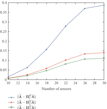
To assess these first results, we performed another study: in place of studying the bias over angle estimation we study the bias over the estimation of Π. We refer to the basic definition of the propagator, that is,A=ΠHA. We compute
Π from all considered methods ((15), (24), and (26)) and for several numbers of sensors. We considered the following error criterion:
e=A−ΠHA, (47)
0 0.2 0.4 0.6 0.8 1 1.2 1.4 1.6
St
d
−20 −15 −10 −5 0 5 10 15 20 SNR (dB)
ΠΓpropagator ΠUpropagator
ΠRpropagator
Figure 4: std of estimation errors as a function of SNR for propagator and modified propagator.
0 0.05 0.1 0.15 0.2 0.25 0.3 0.35 0.4
10 12 14 16 18 20 22 24 26 28 30 Number of sensors
A−ΠHΓA
A−ΠHUA A−ΠH
RA
Figure5: Error obtained with different propagator operators as a function of the number of sensors.
ΠR is represented in Figure 5. The main outcome of this figure is that whatever the number of sensors, the error obtained with LU or QR-based factorization techniques is lower than the one obtained with the spectral matrix-based technique. QR-based factorization technique gives slightly better results compared to LU-based factorization technique, especially for low SNR values (less than –10 dB).
This confirms that better estimation ofΠleads to better estimation of angles.
Note that during our simulations, in order to verify that the information about the source localization is totally
0 0.1 0.2 0.3 0.4 0.5 0.6 0.7 0.8
St
d
2 4 6 8 10 12
Parametermvalue
Figure6: std value obtained with EG method with variable value of parametermandP=8.
confined in the matricesUorR, we have used the lower unit triangular matrixL,instead of the matrixU,with several high SNR values. Our conclusion is that the lower matrix cannot be used to localize the sources.
7.2. Experiment 2: Ermolaev and Gershman algorithm
In this experiment, we first justify the choice of parameter m involved in EG method, and we then study its performance in terms of accuracy of source localization and robustness to noise. The number of sources is taken equal to 8 as in experiment 1.
7.2.1. Choice of parameter m value
We performed a specific study concerning the EG method: in the current experimental conditions, with SNR = 0 dB, we vary the value of parameter m (see (34)). We use QR factorisation and we will keep the same conclusions while using further LU decomposition. The std value over the estimation of source DOAs is decreasing until m = 10 and is then steady (Figure 6). Then, we deduce that the best compromise between reliability of DOA estimation and computational load is reached by choosing m = 10, in the considered experimental conditions. This result is in accordance with studies performed in [6,7,23].
7.2.2. Performance of EG method for source localization
In order to compare the performance of the considered algorithms based on our thresholdsλU
s or λRs to one based on the threshold valueλsarbitrarily chosen betweenλPand λP+1as suggested by [10], several experiments with the same
0 0.5 1 1.5 2 2.5 3
St
d
−10 −5 0 5 10 15 20 SNR (dB)
λs
ProposedλU S
ProposedλR S
Figure7: std of estimation errors as functions of SNR when the spectra of EG algorithm is used withm=10.
0 0.1 0.2 0.3 0.4 0.5 0.6 0.7 0.8 0.9 1
Localization
functions
0 10 20 30 40 50 60 70
Azimth (deg)
λU S λs
Figure8: EG algorithm as a function of the threshold valuesλU S and
λswithm=10 and SNR= −5 dB.
threshold values lead to better results for all SNR values. Figures8and9exemplify the obtained localization results.
The good performances of the proposed modified EG method are reached thanks to the estimation of the number of sources using diagonal elements and the proposed thresh-old values. The results obtained show that the rank revealing triangular factorizations improve DOA localization. This can be explained as follows.
In [7], the approximation of (19) depends strongly on the thresholdλsbetween signal subspace and noise subspace eigenvalues of the spectral matrix.
0 0.1 0.2 0.3 0.4 0.5 0.6 0.7 0.8 0.9 1
Localization
functions
0 10 20 30 40 50 60 70
Azimth (deg)
λR S λs
Figure9: EG method as a function of the threshold valuesλR S and
λswithm=10 and SNR= −5 dB.
Supposing that P is the correct number of sources, choosing a value of λs which is too close to λp induces the overestimation of noise subspace dimension as signal subspace vectors may be included in the noise subspace, which leads to the degradation of the localization using the EG algorithm.
Now, ifP is chosen inadequately, std increases. Indeed several simulations have shown the following behavior. If the number of sources is underestimated the estimated DOA values are uncorrect and if the number of sources is overes-timated one observes unexpected DOA values depending on the experiment.
Then, the problem of the estimation ofλsrequired in EG algorithm could be solved thanks to LU or QR factorizations of the spectral matrix.
7.3. Experiment 3: Fixed-point algorithm and MUSIC
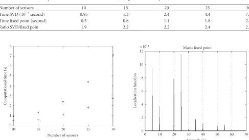
We exemplify the proposed fixed-point algorithm with source localization based on MUSIC method. Several exper-iments with the same experimental conditions as in the previous subsections are carried out with various numbers (seeFigure 10andTable 1,N=20 up to 250) of sensors, to study the computational load of the proposed algorithm as a function of the antenna size. Parameterδis fixed to 10−6and SNR to 0 dB withP=8 sources. DOA values are 5◦, 10◦, 20◦, 25◦, 35◦, 40◦, 50◦, and 55◦.
Table1: Computational time needed to run MUSIC, using SVD and fixed point, for various numbers of sensors.
Number of sensors 10 15 20 25 30
Time SVD (10−2second) 0.95 1.3 2.4 4.4 7.1
Time fixed point (second) 0.5 0.6 1.1 1.8 2.8
Ratio SVD/fixed poin 1.9 2.2 2.2 2.4 2.5
0 1 2 3 4 5 6 7 8
C
o
mputational
time
(s)
10 15 20 25 30
Number of sensors
Figure10: Computational time for MUSIC with SVD (·) and for MUSIC with fixed-point algorithm (+).
0 2 4 6 8 10 12 14 16 18 ×1015
Localization
function
0 10 20 30 40 50 60 70
Azimuth (◦) Music SVD
Figure11: Pseudospectrum of MUSIC obtained using SVD.
Figure 10and Table 1 show that MUSIC method with fixed-point algorithm is up to 2.5 faster than MUSIC method using SVD.
7.4. Experiment 4: Performance of noneigenvector methods
In this experiment, we study the robustness to noise of propagator and of the EG method both using QR
factoriza-0 2 4 6 8 10 12 ×1014
Localization
function
0 10 20 30 40 50 60 70
Azimuth (◦) Music fixed point
Figure12: Pseudospectrum of MUSIC obtained using fixed point.
0 0.2 0.4 0.6 0.8 1 1.2 1.4
St
d
−10 −5 0 5 10 15 20 SNR(dB)
Figure 13: Standard deviation values for various SNR values obtained with noneigenvector EG method (+), MUSIC method (∗), propagator method (o), Cram´er Rao bound (∗-).
tion of the accelerated MUSIC algorithm. Indeed we noticed (see Figures4and7) that the results obtained are the best when QR factorization is used. Moreover, using fixed-point algorithm in place of SVD does not alter the results in terms of performance.
Cram´er-Rao bound for MUSIC method (which exhibits the lowest Cram´er Rao bound values).
We used the formulas provided in [27].
7.5. Performance in the estimation of the number of sources
In the algorithms studied in this paper, one major point is the estimation of the number of sources.
The accuracy of DOA estimation is conditioned by the correct estimation of the number of sources.
We proposed (36) to estimate the number of sources. This method was tested with several simulations, and we validated this criterion for several values of number of sources and SNR values.
In all simulations, we retrieve the correct number of sources.
8. CONCLUSION
In this paper, we have improved two noneigenvector high-resolution methods, namely, the propagator method and the Ermolaev and Gershman algorithm. We proposed a noneigenvector version of MUSIC algorithm, replacing singular value decomposition by fixed-point algorithm. The improvement of the propagator method and Ermolaev and Gershman algorithms is based on LU or QR factorization of the spectral matrix. This leads to an efficient local-ization of the narrow-band sources even if the SNR is low. Actually, the upper triangular matrices contain the information enabling source localization. We have modified the existing methods to estimate the number of sources based on eigenvalues by introducing the diagonal elements of the upper triangular matrix. The existing propagator method is a least square solution and still very sensitive to noise. On the opposite, the modified propagator method is calculated accurately from the upper triangular matrix even in the presence of noise. A major problem of the Ermolaev and Gershman algorithm is the estimation of the threshold. New and analytical thresholds are proposed to apply Ermolaev and Gershman algorithm. The threshold values are estimated thanks to the norm of the block matrix of the upper-right corner triangular matrix. The resulting algorithm for the localization without eigendecom-position is an approximation method, but the numerical results show its high accuracy even when the SNR is low. By adapting fixed-point algorithm for the estimation of leading eigenvectors, we obtained a noneigenvector source localization method. MUSIC algorithm has been shown to be up to 2.5 times faster with this improvement. We compared the performances of the three proposed noneigenvector methods, propagator and EG and MUSIC using fixed-point algorithm, by providing std evolution for several SNR values. MUSIC and propagator yield close std results. MUSIC with fixed-point algorithm has the smallest computational load and exhibits the best perfor-mance.
ACKNOWLEDGMENT
The authors would like to thank the reviewers for their care-ful reading and their helpcare-ful comments which contributed to improve the quality of the paper.
REFERENCES
[1] R. O. Schmidt, “Multiple emitter location and signal param-eter estimation,”IEEE Transactions on Antennas and Propaga-tion, vol. 34, no. 3, pp. 276–280, 1986.
[2] G. Bienvenu and L. Kopp, “Optimality of high resolution array processing using the eigensystem approach,”IEEE Transactions on Acoustics, Speech, and Signal Processing, vol. 31, no. 5, pp. 1235–1248, 1983.
[3] S. Bourennane and A. Bendjama, “Locating wide band acous-tic sources using higher order statisacous-tics,”Applied Acoustics, vol. 63, no. 3, pp. 235–251, 2002.
[4] T.-H. Liu and J. M. Mendel, “Cumulant-based subspace tracking,”Signal Processing, vol. 76, no. 3, pp. 237–252, 1999. [5] J. Munier and G. Y. Delisle, “Spatial analysis using new
properties of the cross-spectral matrix,”IEEE Transactions on Signal Processing, vol. 39, no. 3, pp. 746–749, 1991.
[6] M. Frikel and S. Bourennane, “High-resolution methods with-out eigendecomposition for locating the acoustic sources,” Applied Acoustics, vol. 52, no. 2, pp. 139–154, 1997.
[7] V. T. Ermolaev and A. B. Gershman, “Fast algorithm for minimum-norm direction-of-arrival estimation,”IEEE Trans-actions on Signal Processing, vol. 42, no. 9, pp. 2389–2394, 1994.
[8] C. H. Bischof and G. M. Shroff, “On updating signal subspaces,”IEEE Transactions on Signal Processing, vol. 40, no. 1, pp. 96–105, 1992.
[9] P. Strobach, “Square-root QR inverse iteration for tracking the minor subspace,”IEEE Transactions on Signal Processing, vol. 48, no. 11, pp. 2994–2999, 2000.
[10] H. Akaike, “Maximum likelihood identification of Gaussian autoregressive moving average models,”Biometrika, vol. 60, no. 2, pp. 255–265, 1973.
[11] J. Rissanen, “Modeling by shortest data description,” Automat-ica, vol. 14, no. 5, pp. 465–471, 1978.
[12] W. Chen, K. M. Wong, and J. P. Reilly, “Detection of the number of signals: a predicted eigen-threshold approach,” IEEE Transactions on Signal Processing, vol. 39, no. 5, pp. 1088– 1098, 1991.
[13] P. Comon and G. H. Golub, “Tracking a few extreme singular values and vectors in signal processing,” Proceedings of the IEEE, vol. 78, no. 8, pp. 1327–1343, 1990.
[14] G. Quintana-Ort´ı and E. S. Quintana-Ort´ı, “Parallel codes for computing the numerical rank,” Linear Algebra and Its Applications, vol. 275-276, pp. 451–470, 1998.
[15] G. H. Golub and V. Loan,Matrix Computations, John Hopkins University Press, Baltimore, Md, USA, 3rd edition, 1996. [16] S. Marcos, A. Marsal, and M. Benidir, “The propagator
method for source bearing estimation,”Signal Processing, vol. 42, no. 2, pp. 121–138, 1995.
[17] S. Bourennane and M. Frikel, “An improved frequency smoothing method for bearing estimation,” in Proceedings of the 1st Forum Acusticum (ACTA ACUSTICA), p. S253, Antwerpen, Belgium, April 1996.
[19] C.-T. Pan, “On the existence and computation of rank-revealing LU factorizations,”Linear Algebra and Its Applica-tions, vol. 316, no. 1–3, pp. 199–222, 2000.
[20] L. Miranian and M. Gu, “Strong rank revealing LU factoriza-tions,”Linear Algebra and Its Applications, vol. 367, pp. 1–16, 2003.
[21] T.-M. Hwang, W.-W. Lin, and D. Pierce, “Improved bound for rank revealing LU factorizations,”Linear Algebra and Its Applications, vol. 261, no. 1–3, pp. 173–186, 1997.
[22] T. F. Chan, “Rank revealing QR factorizations,”Linear Algebra and Its Applications, vol. 88-89, pp. 67–82, 1987.
[23] J. Choi, I. Song, and H. M. Kim, “On estimating the direction of arrival when the number of signal sources is unknown,” Signal Processing, vol. 34, no. 2, pp. 193–205, 1993.
[24] D. Stott Parker, “Schur complements obey Lambek’s categorial grammar: another view of Gaussian elimination and LU decomposition,”Linear Algebra and Its Applications, vol. 278, no. 1–3, pp. 63–84, 1998.
[25] N. J. Higham, “QR factorization with complete pivoting and accurate computation of the SVD,” Linear Algebra and Its Applications, vol. 309, no. 1–3, pp. 153–174, 2000.
[26] A. Hyv¨arinen and E. Oja, “A fast fixed-point algorithm for independent component analysis,”Neural Computation, vol. 9, no. 7, pp. 1483–1492, 1997.
[27] P. Stoica and A. Nehorai, “MUSIC, maximum likelihood, and Cram´er-Rao bound: further results and comparisons,”IEEE Transactions on Acoustics, Speech, and Signal Processing, vol. 38, no. 12, pp. 2140–2150, 1990.
[28] F. Li and R. J. Vaccaro, “Unified analysis for DOA estimation algorithms in array signal processing,”Signal Processing, vol. 25, no. 2, pp. 147–169, 1991.