Modelling and optimising the sport and exercise training process

EXERCISE TRAINING PROCESS

PhD Thesis

MANSOUR SHRAHILI

Universtity of Salford, Salford, UK

LIST OF CONTENTS...I

LIST OF FIGURES...IV

LIST OF TABLES...VII

DECLARATION...IX

ABSTRACT...X

1. INTRODUCTION...1

1.1 Objectives of research...1

1.2 The relationship between training and performance...2

1.3 The components of training...3

1.4 Overtraining symptoms...3

1.5 Summary and structure...4

2. THE STUDY DATA...6

2.1 Training data...6

2.2 Heart rate measurement...8

2.3 Power output...9

3. MEASURING TRAINING AND PERFORMANCE...14

3.1 Introduction...14

3.2 Measuring training...14

3.2.1 Training load for a session: Training impulse (TRIMP)...14

3.2.2 The accumulation of training (Banister model)...16

3.3 Measuring performance...19

3.3.1 Introduction...19

3.3.2 A new measure of performance...20

3.4 Summary...28

4. DETERMINING THE PARAMETERS OF THE ACCUMULATED TRAINING EFFECT...29

4.1 Introduction...29

4.2 Estimating the Banister model parameters...30

4.3 Determining starting values of our model...31

4.4 Pre-processing the data...32

4.5 Results...32

4.6 The significance of the training effect...43

4.6.1 The statistical significance of the training effect...43

4.6.2 The practical significance of the training effect...43

4.7 Discussion of results...46

4.8 Optimising training...48

4.9 Summary...48

5. OTHER MEASURES OF PERFORMANCE...49

5.1 Average power (AP)...49

5.2 Normalised power (NP)...49

5.3 Critical power (CP)...51

5.3.1 The Akaike Information Criterion (AIC)...52

5.4 Another measure of performance based on the critical power concept...53

5.4.1 Modelling the critical power...53

5.4.2 Models of critical power with CP varying by rider and by session...55

6.1 Summary and conclusion...77

6.2 Main findings...77

6.3 Implications...78

6.4 Limitations of the work...78

6.5 Future work...79

Appendix 1 Correlations for power output against heart rate at different lags...80

Appendix 2 Power output against heart rate for all sessions for all riders...98

Appendix 3 Correlations of the ATE and performance measure for various parameter values...140

Figure 1.1 The influence of training over a period of time...3

Figure 2.1 The number of sessions and the period in day for each rider’s training schedule6 Figure 2.2 An example of power output (Watts) and heart rate (beats per minute, bpm) from a single session for one rider...7

Figure 2.3 A chest-worn heart-rate monitor...8

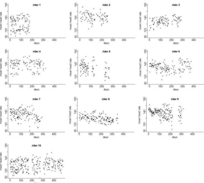
Figure 2.4 Mean heart rates for each session for each rider...9

Figure 2.5 An example SRM power meter crank. This is the SRM Canondale MTB 2x10 model, which weighs 521g and costs €1892 (SRM, 2012)...10

Figure 2.6 An example SRM data recorder and display. This is the Power Control 7 model, with a battery life of 120 hours (SRM, 2012)...10

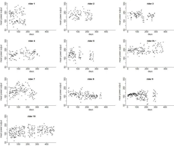
Figure 2.7 Mean power outputs (Watts) for each session for each rider...11

Figure 2.8 The histograms of heart rate data (all sessions) for each rider (1-10)...12

Figure 2.9 The histograms of power output (all sessions) for each rider (1-10)...13

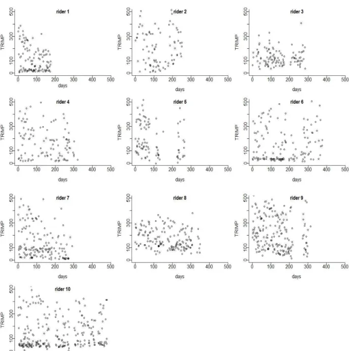
Figure 3.1 Training impulse (TRIMP) for each rider for each session using Borresen and Lambert constants...16

Figure 3.2 The components of the Banister model...18

Figure 3.3 An example of the Banister curve for a single session with default parameters ( τ_a=3days , τ_f=2days , k_a=1∧k_f=1.3_)...18

Figure 3.4 An example of the Banister curve for a progressive training schedule of 200 days with unit training load for each session, and with parameters as τ_a=3days , τ_f=2days , k_a=1∧k_f=1.3_{, (plot A) and} τ_a=20days , τ_f=10days , k_a=1∧k_f=1.3 _{(plot B).}...18

Figure 3.5 Another example of the Banister curve for an every other day training schedule over 200 days with unit training load for each session, and with parameters as τ_a=3days , τ_f=2days , k_a=1∧k_f=1.3_{, (plot A) and} τ_a=20days , τ_f=10days , k_a=1∧k_f=1.3_{, (plot B).}...19

Figure 3.6 Power output against heart rate for a single session with lag =15 seconds...20

Figure 3.9 The performance measure for a single session for rider 3...25

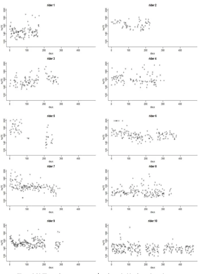
Figure 3.10 The performance measure hP75 for each rider for each session...27

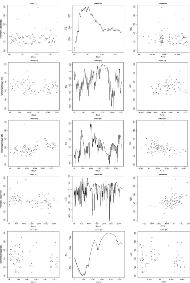
Figure 4.1 Performance measure hP50and the curve of the accumulated training effect over

time for each rider when kf=2...34

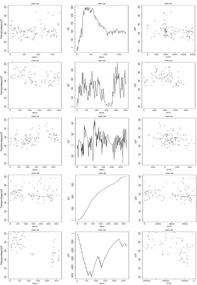
Figure 4.2 Performance measure hP75 and the curve of the accumulated training effect over

time for each rider when kf=2...36

Figure 4.3 Performance measure hP50and the curve of the accumulated training effect over

time for each rider when kf≠2...39

Figure 4.4 Performance measure hP75and the curve of the accumulated training effect over

time for each rider when kf≠2...41

Figure 5.1 An example of average power ( ) and normalised power ( ) with underlying power measurements sampled every 5 seconds during a single session...50

Figure 5.2 Normalised power (NP) against average power (AP) for all riders (1 to 10)....51

Figure 5.3 The concept of critical power...52

Figure 5.4 Fixed levels of intensity (Watts) versus duration (5 seconds) for one session for each rider (1 to 10)...56

Figure 5.5 Critical power curve for each rider for all sessions with fitted minimum AIC fixed effects model with unit of duration (5 seconds) and unit of power (Watts)...60

Figure 5.6 The parameter estimates p0 for each session for each rider ± 2 standard errors61

Figure 5.7 p0 varying by session for all riders...63

Figure 5.8 p0 varying by session and smoothing curves for p0, plotted against day for all

riders (1 to 10)...65

Figure 5.9 Critical heart rate curve for each rider for all sessions with fitted fixed effects model with minimum AIC fixed effects model with unit of duration (5 seconds) and unit of heart rate (beats per minute)...69

Figure 5.10 The parameter estimates h0 for each session for each rider ± 2 standard error70

Figure 5.11 h0varying by session for all riders...72

Figure 5.12 h0varying by session, and smoothing curves for h0 plotted against day for each

Figure 5.14 p0/h0versus day for each rider with smoothing degree = 0.1 ( ), and

Table 2.1 Age, height and weight of the ten riders...6

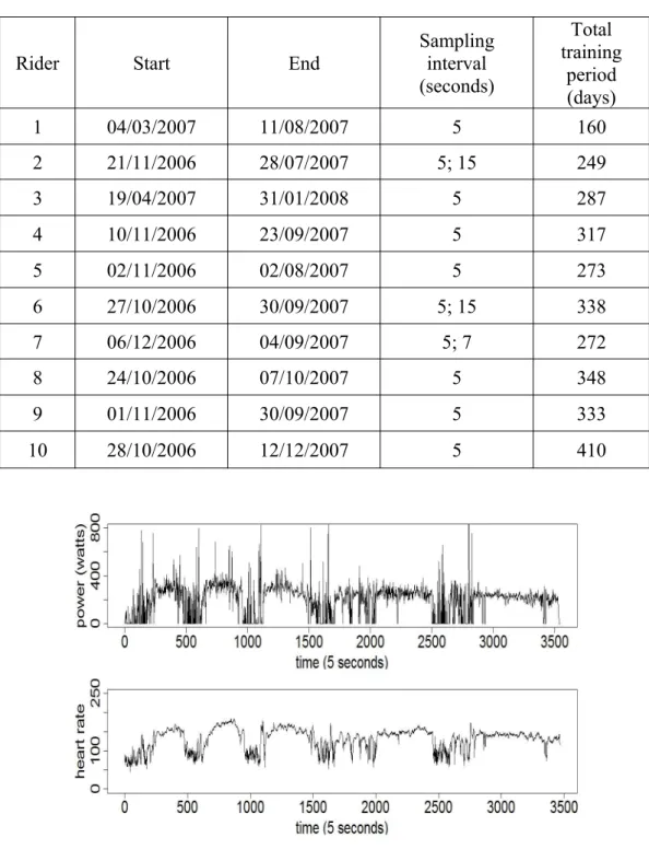
Table 2.2 Start date, end date and duration of training schedules for each of the 10 riders. .7

Table 3.1 Maximum and resting heart rate (beats per minute) for each rider...15

Table 3.2 Sample linear correlation between power output and heart rate for each session for rider 3 with different heart rate lags of seconds (0, 10, 15, 20, and 30 seconds), the strongest correlation for each session is highlighted...21

Table 3.3 Selected percentiles of power output for each rider...26

Table 4.1 The initial parameter values for the Banister model with the correlation between the performance measure and the accumulated training effect (ATE)...32

Table 4.2 Parameter estimates of the model (standard errors) when k_f=2 for performance measure hP50...33

Table 4.3 Parameter estimates of the model (standard errors) when k_f=2 for performance measure hP75...33

Table 4.4 Parameter estimates of the model (standard errors) when k_f≠2 for performance measure hP50...38

Table 4.5 Parameter estimates of the model (standard errors) when k_f≠2 for performance measure hP75...38

Table 4.6 The coefficients of the linear model between power output and heart rate

calculated from the last two months for each rider with the standard error...44

Table 4.7 The accumulated training effect change and performance gain for each rider when kf=2and for performance measure hP50...44

Table 4.8 The accumulated training effect change and performance gain for each rider when kf=2and for performance measure hP75...45

Table 4.9 The accumulated training effect change and performance gain for each rider when kf≠2 and for performance measure hP50...45

Table 4.10 The accumulated training effect change and performance gain for each rider when kf≠2 and for performance measure hP75...45

Table 5.1 The correlation between average power (AP) and normalised power (NP) for all riders...50

Table 5.4 Fitted models of heart rate with their AIC and maximum likelihood values...66

In elite sport, the fundamental aim of training is to improve performance in competition. It should develop the abilities of the athletes to achieve the highest level of performance. The fundamental aim of monitoring in training is to determine whether training is appropriate for an athlete and whether training should be modified. Broadly, the purpose is to control the training program of an athlete to ensure that the maximum level of performance by the athlete is reached at a known competition at a known time in the future.

1.1 Objectives of research

This thesis is concerned with modelling the training process in sport and exercise, and in cycling in particular. Our purpose is to provide a quantitative model that can be used to optimise training in advance of a major competition. An optimal training program would prevent under-training, overtraining and injury (Meeusen, et al., 2006).

Training is the method by which an athlete improves his or her specific performance and develops individual characteristics according to the requirements of a specific competition (Yin, et al. 2010). Smith (2003a) stated that the training process involves repetition of exercises designed to develop the skills of a rider that lead to increased physical performance. The principal aim of cycling training is to improve and increase the ability of a rider to sustain a power output or speed for a given distance or time.

Training should be balanced. It should support the rider and develop his or her capabilities and allow the athlete to gain the right amount of training. If a rider trains too much, he may get injured or sick but if he trains too little he may get little benefit. Measuring and monitoring the positive and negative effects of training will help coaches and athletes to design their training program in order to maximise performance at a specific time. So, training strategy should be developed to achieve peak performance. To do this, very hard riding and the correct amount of recovery must be combined (Faria, et al., 2005), so that over-training and injury or illness inducing fatique can be avoided (Smith, 2003b). This trade-off between under and over-training was first discussed by researchers in the former East Germany and later developed by Banister et al. (1975). Our purpose is to use a quantitative approach to find the optimum balance between under and over-training. To do so, we develop a statistical model to relate training to performance. To do this, both training and performance must be measured, and we do so using field data relating to power output and heart-rate. This research is the first to use field data to model training and performance in this way.

Ultimately, we intend that measures of training and performance and the statistical model that links them will be used to optimise training: that is, used to determine the training schedule that maximises the performance of an athlete on a particular day in the future. Such a schedule would require a rider to carry out particular tasks at particular times. In practice and theory the schedule would have to be adaptive.

The measure of training we use is an established one based on the concept of accumulated training load; this is broadly an exponentially weighted moving average of the total load on the cardio-vascular system during training of a rider over all time. However, this accumulated training load measure depends on a number of unknown parameters that must be specified for an individual athlete; only then can training be theoretically optimized for this specific athlete.

the accumulated training load measure such that this measure is most closely related to the performance measure. We will explore other measures of performance but ultimately this performance measure is our preferred measure.

Mathematical models of training exist, but it has proved difficult to implement these in a practical context so that training schedules might be optimised. The optimal training strategy to improve functional strength in cycling is still unclear and current practice is rather based on the experience and perception than on sound scientific evidence (Koninckx, et al. 2010). As a result, current practice of training riders relies upon riders' and coaches' intuition and experience, with only limited support from quantitative analyses. This thesis will explore the optimisation of training through the analysis of a large dataset on power output and heart-rate of competitive cyclists.

1.2 The relationship between training and performance

The relationship between training and performance is very important for coaches who look to determine a training program for their riders. Research that has investigated this relationship by using quantitative data can be traced back to the seminal work of Banister, et al. (1975). However, in spite of the time that has elapsed since these early ideas were described, predicting the results of a particular training program is difficult, and in particular predicting performance output from training input remains an unsolved problem (Jobson, et al. 2009). The relationship between training and performance is highly individualised because of a number of factors (Avalos, et al. 2003). These factors include genetic factors, individual training background, psychological factors, technical factors and speciality, and they are very difficult to quantify (Hellard, et al. 2006; Jobson, et al. 2009). However, positive relationships between training and performance and between higher training intensity and performance have been found for individual sports such as swimming and running (Gabbett and Domrow, 2007).

The amount and type of training can positively affect the physical capabilities of a athlete. On the other hand, an athlete is negatively affected by the amount of fatigue that the training itself accumulates in the athlete (Banister, et al. 1975). Qualitative predictions and descriptions of the effect of training have been made. For example, one can observe a rapid improvement in performance when the initial performance is low, but as an athlete becomes fitter and better trained, it becomes more difficult to observe further improvement in performance by continued or more intensive training.

performance. However, a random increase in training volume, intensity or frequency may lead to over-training which increases the likelihood of injury.

Avalos, et al., (2003) have discussed the effect of training on performance of 13 elite swimmer over three seasons. They reported significant changes in the impact of training on performance from the first to the third season. The effect of training on performance has been studied in different sports (Millet, et al., 2002), including running (Banister and Hamilton, 1985; Banister, et al., 1986) and swimming (Avalos, et al., 2003; Mujika, et al., 1996). The purpose of this study is to relate training to performance using data collected in the field using a power meter and heart-rate monitor.

1.3 The components of training

Banister et al. (1975) proposed a model that describes the influence of training on performance at any time t. They suggested that in its simplest form, the influence of training is the difference between two components. These components are fitness, which is the positive influence of training, and detriment, which is the negative influence of training. Throughout the training period, the level of training (or readiness to perform) is described as the difference between the accumulated fitness (benefit) and the accumulated detriment (dis-benefit), see figure 1.1. Training load is a combination of three elements. They are intensity, duration and frequency (Smith, 2003a).

Figure 1.1 The influence of training over a period of time.

1.4 Overtraining symptoms

fatigue and then progress to severe symptoms such as sleep problems and lack of motivation (Jeukendrup and Diemen, 1998), so it is important for coaches and athletes to identify overtraining as early as possible to modify training before getting reduction in the athlete’s performance.

The number of overtraining symptoms is large (Gleeson, 2002). Fry, et al. (1991) reported over 200 symptoms. Mackinnon, (2000) and Halson and Jeukendrup, (2004) listed some overtraining symptoms as persistent and severe fatigue, poor and declining performance in sport with continued training and frequent illness. In addition, decreased maximum heart rate, decreased oxygen uptake and decreased lactate levels have also reported as overtraining symptoms (Hassmén and Kenttä, 1998) and (Lehman, et al. 1993). However, heart rate monitoring could be used to discover overtraining at early stages and prevent it (Jeukendrup and Diemen, 1998).

There are many causes that can lead to overtraining symptoms. However, there is no single objective marker to identify overtraining syndrome (Mackinnon, 2000). Halson and Jeukendrup, (2004) mentioned that a number of investigations have been carried-out to test the effects of an intensified training period that can lead to overtraining. One of the most important reasons for overtraining symptoms is a dramatic increase of training or competition intensity with insufficient time for recovery (Smith, 2003b; Lehman, et al. 1993; Fry and Kraemer, 1997). Sudden increase in training volume and/or intensity, a heavy competition schedule and monotonous training program are also reported as causes of overtraining (Mackinnon, 2000). Weeks to months of complete rest are required to recover from overtraining symptoms (Mackinnon, 2000).

1.5 Summary and structure

To summarise, the purpose of this thesis is to develop a statistical model that relates training to performance for a particular rider. Training can then be scheduled to maximise performance at a particular competition. This thesis is structured as follows.

In chapter two, we describe the athletes, their data, and how the data were collected. These data are power output and heart rate collected every five seconds for the sessions (training and competition) of ten riders over a period of time. We plot examples of the power output and heart rate series for a number of sessions. In the final part of this chapter, we present the entire history of power output and heart rate data for each rider.

Chapter three discusses the measurement of training and performance. We use in this chapter a measure of training load for a session called the training impulse (TRIMP). Then, we explain the Banister model (proposed by Banister et al. 1975), which is used to measure the accumulation of training given known parameters of the model. The quantified accumulation of training is called the accumulated training effect (ATE). The next part of this chapter describes our performance measure. This measure is based on the relationship between power output and heart rate. Power is related to heart-rate using the entire history of sessions for each rider. In particular, in this relationship, we use a 15 second time-lag between power output and heart rate, and justify this choice of lag.

training effect. We briefly describe how the estimated parameters can then be used to optimise training.

Chapter five summarises some other possible measures of performance, such as average power, normalised power, critical power and a measure based on the concept of the critical power that might be used to determine the Banister model parameters.

2. THE STUDY DATA

2.1 Training data

Training data from a number of competitive riders were available to us. These cyclists gave written, informed consent for their data to be used in our study. The study received local ethical committee approval and was carried out according to the principles of the Declaration of Helsinki (World Medical Association, 2013). For each rider, for a number of training sessions typically extending over a 300 day period between December 2006 and September 2007, power output and heart-rate were recorded every five seconds. In the current study, riders are numbered to maintain their anonymity and privacy. The ten riders have mean (standard deviation) age of 36 (9) years, height of 1.79 (0.46) metres, and weight of 74.3 (6.8) kg. The age (years), height (metres) and weight (kilograms) of each rider are shown in Table 2.1. A summary brief description of our data is given in Figure 2.1, Table 2.2 and Figure 2.2. According to Figure 2.1, there is variation among the ten athletes. Each athlete has trained or approximately 50% of the total number of days. Missing data for a particular day might be due to either a lack of recording or there being no ride that day.

Table 2.1 Age, height and weight of the ten riders

Rider Age

(years)

Height (m)

Weight (kg)

Rider Age

(years)

Height (m)

Weight (kg)

1 45 183.0 74.3 6 27 183.7 71.8

2 52 175.0 74.5 7 40 177.5 75.5

3 35 181.0 71.0 8 34 182.0 77.0

4 _{42 178.5 78.2} 9 _{34 185.5 88.2}

5 _{21 171.4 60.9} 10 _{29 174.5 71.5}

Table 2.2 Start date, end date and duration of training schedules for each of the 10 riders

Rider Start End Samplinginterval

(seconds)

Total training

period (days)

1 04/03/2007 11/08/2007 5 160

2 21/11/2006 28/07/2007 5; 15 249

3 19/04/2007 31/01/2008 5 287

4 10/11/2006 23/09/2007 5 317

5 02/11/2006 02/08/2007 5 273

6 27/10/2006 30/09/2007 5; 15 338

7 06/12/2006 04/09/2007 5; 7 272

8 24/10/2006 07/10/2007 5 348

9 01/11/2006 30/09/2007 5 333

10 28/10/2006 12/12/2007 5 410

Figure 2.3 An example of power output (Watts) and heart rate (beats per minute, bpm) from a single session for one rider

was developed after the data were collected. Therefore, we plan our method according to the available data.

2.2 Heart rate measurement

Heart rate measurement is one of the most popular methods of measuring exercise intensity during a training session. It is measured in beats per minute. Nimmerichter, et al. (2011) mentioned that many studies have used heart rate as a measure of estimating exercise intensity in a variety of sports such as cycling (Lucia, et al. 1999); running (Gilman and Wells, 1993); tennis (Therminarias, et al. 1991); and soccer (Ali and Farrally, 1991). Many researchers referred the basis of this method to the established linear relationship between heart rate and steady-state work rate (Hopkins, 1991; Arts and Kuipers, 1994; Robinson, et al. 1991). There are many devices available that can monitor the heart rate of an athlete when he does exercise (figure 2.3). These monitors have been widely used for different sports over the last two decades (Achten and Jeukendrup, 2003). They are used to determine the exercise intensity of a training session or race. The exercise intensity of a session is one of the most important applications of heart rate monitoring (Achten and Jeukendrup, 2003). These devices can help coaches and athletes to monitor and plan the athletes’ training intensity. The first telemetric monitors of heart rate were invented in 1982 and then developed to store heart rate data (Lambert, et al. 1998). These data can be transferred to a computer in order to analyse them and get some information about an athlete. The use of heart rate monitors has been studied in many sports such as cycling, running and soccer (Lambert, et al. 1998). The mean heart rates for each session for each rider are shown in figure 2.4.

Figure 2.5 Mean heart rates for each session for each rider

2.3 Power output

Figure 2.6 An example SRM power meter crank. This is the SRM Canondale MTB 2x10 model, which weighs 521g and costs €1892 (SRM, 2012).

3.1 Introduction

In this chapter, we explain our method for relating training to performance. In order to do this, both training and performance must be measured. We will give a brief explanation of measuring training and measuring performance. We use data on power output and heart rate collected every five seconds during training. The next chapter will then explain how to relate one to the other.

3.2 Measuring training

Banister, et al. (1975) proposed a measure of training that calculates the accumulative effect of all training carried out up to time t. This measure had a number of components. The first one is the measurement of the amount of training for a single session, called the training load of that session. In general, training load of a session can be written as average intensity × duration. In this thesis, we use training impulse (TRIMP) as a measure of the training load for a session. The second component is how training accumulates for a sequence of sessions over time. In the next subsections we will explain these components in detail.

3.2.1 Training load for a session: Training impulse (TRIMP)

The training impulse (TRIMP) is a measure that calculates how hard a rider trains in a single session. The concept of training impulse combines training intensity and training duration into a single measure to provide higher weighting for higher intensity sessions (Akubat and Abt, 2011). This measure is based on heart rate measurements during training (Joosen, et al., 2013). The training impulse (TRIMP) has been used as an indicator of training load during training and competition by several researchers (Morton, et al., 1990; Padilla, et al., 2000). Recently, it has been used for describing training load in professional road cycling to plan training in an appropriate way (Padilla, et al., 2000; Padilla, et al., 2001).

The concept of training impulse was first presented by Banister, et al. (1975) and Banister and Calvert, (1980) as follows

TRIMP=T × H

where T is the training time in minutes of the session and H is the average heart rate of the session (beats per minute). Thus, here, TRIMP is the total number of heart beats during a session. However, using the above formula to calculate TRIMP does not reflect the overall intensity of a session (Akubat and Abt, 2011; Stagno, et al., 2007).

The original formula was modified by Morton, et al. (1990) to include a multiplicative factor that gave greater weight to high-intensity training and it is defined as follows

TRIMP=T × a× Hratioe b Hratio

H_ratio=

(

)

T is the duration of exercise and HR_ex is the average heart rate during the exercise and

HR_rest is the resting heart rate (the number of heart beats per minute). HR_rest should be calculated upon waking and while still lying in bed. The fitter the rider, the lower is his resting heart rate. HR_max is the maximal heart rate. Table 3.1 presents the maximum heart rate and the resting heart rate for each rider in our study. These data are recorded in our dataset. The constant ais taken to be 0.64 for males and 0.86 for females (Borresen and Lambert, 2009). The constant b is based on blood lactate and it is taken to be 1.92 in males and 1.67 in females.

There are conflicting views about the values of the TRIMP parameters. The study of Stagno et al (2007) have reported the constants a and b as being 0.1225 and 3.94 for males respectively. They plotted the blood lactate concentration of 8 participants against the fractional elevation in heart rate, and then estimated them by fitting an exponential line.

Figure 3.1 shows the training impulse (TRIMP) for each rider for each session using

a=0.64, b=1.92.

Table 3.3 Maximum and resting heart rate (beats per minute) for each rider

Rider H_max H_rest Rider H_max H_rest

1 180 45 6 187 39

2 203 48 7 187 49

3 182 45 8 173 42

4 192 42 9 192 53

Figure 3.11 Training impulse (TRIMP) for each rider for each session using Borresen and Lambert constants

3.2.2 The accumulation of training (Banister model)

strength. Calvert, et al. (1976) simplified this model to two components which are fitness and detriment.

Hellard, et al. (2006) mentioned some limitations to the Banister model approach. These limitations are “the limited accuracy of the model to predict future performance; the difference between estimated and actual changes in performance; and the poor corroboration of the model with physiological mechanisms" (Hayes and Quinn, 2009). Moreover, this model has many parameters which are hard to estimate especially with noisy data. Additionally, missing data will affect the accumulation of training.

The Banister model has been applied for several sports such as running (Morton, et al., 1990; Wood, et al., 2005), swimming (Hellard, et al., 2006; Hellard, et al., 2005; Mujika, et al., 1996), weight lifting (Busso, et al., 1990) and cycling (Busso, 2003; Busso, et al., 2002; Busso, et al., 1991; Busso, et al., 1997). It has been commonly used to describe the dynamics of training (Hellard, et al., 2005). We will discuss in detail what they have done in the next chapter.

The Banister model defines the accumulated training effect at time t of training sessions occurring up to time t as

W(t)=w₀+k_a

∑

i=1

nt

w_sie−(t−si)/τa−k

f

∑

nt

w_sie−(t−si)/τf (3.1)

where W(t) is the accumulated training effect (ATE) at time t . This can then be

interpreted as the readiness-to-perform at time t and hence represents the potential performance at time t. s_i is the time at which session i was completed. wsi is the known

training load during session iwhich is the amount of training that a rider completed during the session (Wallace, et al. 2013). It is defined as a function of h_i where h_iis the heart rate history for session i alone. One possible candidate for training load is training impulse (TRIMP) which was defined previously. n_t is the number of sessions up to time t. w₀

corresponds to the net training effect at time t=0 of sessions in

(

]

w_sie−(t−si)/τa

the training benefit at time t of a session i that took place at time si<t and w_sie−(t−si)/τf

the training detriment (fatigue) at time t of a session i that took place at timesi. Critically, it is the training benefit and training detriment that must be quantified in order to optimise training (Hayes and Quinn, 2009; Taha and Thomas, 2003). The benefit and detriment associated with a particular session decay at different rates depending on the parameters τ_a and τ_f, the fitness and detriment decay time constants, respectively. The decay in both fitness and detriment is assumed to be exponential and in principle, the decay of fitness is slower than the decay of detriment: τ_a>¿τ_f. k_a and k_f are the scale constants that control the relative size of the immediate training benefit with respect to the immediate training detriment. Strictly, one or other of these parameters is redundant as the scale of

W(t) is arbitrary. Therefore, without loss of generality we will set ka=1 throughout. Thus W(t) in equation (3.1) is the resultant accumulation of decaying benefits and detriments over time.

Figure 3.12 The components of the Banister model

In this study, as the Banister model is a nonlinear model we need more data points per parameter than for a linear regression model. This means a large number of observations would be required to use suitable statistical analysis and to get accurate results. An example of the Banister curve for the response to a single session is shown in figure 3.3 with default parameters. Figure 3.4 shows the Banister curve for a progressive training schedule of 200 days with unit training load for each session, and with parameters as in figure 3.3. For a different type of training schedule with similar parameter values of the Banister model see figure 3.5.

Figure 3.13 An example of the Banister curve for a single session with default parameters (

τ_a=3days , τ_f=2days , k_a=1∧k_f=1.3)

τ_a=3days , τ_f=2days , k_a=1∧k_f=1.3, (plot A) and

τ_a=20days , τ_f=10days , k_a=1∧k_f=1.3, (plot B).

Figure 3.15 Another example of the Banister curve for an every other day training schedule over 200 days with unit training load for each session, and with parameters as

τ_a=3days , τ_f=2days , k_a=1∧k_f=1.3, (plot A) and

τ_a=20days , τ_f=10days , k_a=1∧k_f=1.3, (plot B).

3.3 Measuring performance 3.3.1 Introduction

Performance can be measured in a standard way by asking an athlete to swim or ride or run (depending on the type of sport) a particular specified distance. It could be practically defined as maximum peak power or speed, or time to exhaustion for a given speed or power (Smith, 2003a). Larson, et al., (2013) stated that ‘In many sports, performance is based on maintaining high-level physical outputs during repeated bouts’. A difficulty with this approach is that performance measurements may be infrequent and they may underestimate actual capability or readiness-to-perform; or the rider may hold something back. However, in our approach we aim to use data from a long period of training in order to measure performance.

Therefore, measuring performance from data on training is potentially useful. We now discuss how to do this. Firstly in the next section we present the measure that we think is most important. Other possible measures are also discussed in chapter five.

3.3.2 A new measure of performance

In this section, we present a new measure of performance based on the relationship between power output and heart rate collected every five seconds for cyclists during riding. We focus firstly on the relationship between power output and heart rate. Then we propose our new measure of performance based on this relationship.

3.3.2.1 The relationship between power output and heart rate

It is generally accepted that power output is proportional to heart rate excess (the difference between heart rate and resting heart rate). For example, Grazzi et al. (1999) investigated the relationship between power output and heart rate for 290 participants including 500 tests conducted. They found a strong correlation of 0.98 or above for many riders. There is also a delay or time lag between the change in power output and the heart rate response. The literature is less clear on the value of this delay or lag. Jeukendrup and Diemen, (1998) argued its existence for periods of exercise of short duration, as the circulatory system is not able to fully adapt to change in exercise intensity. However, the size of the lag was not indicated. Stirling, et al. (2008) suggested that for both increases and decreases in heart-rate, these changes in heart rate (e.g. 80 to 160 beats per minute) occur over a period of approximately 30-60 seconds. For the data in our study, short term changes in heart-rate tend to be smaller than in the Stirling et al. study. We speculate that for sessions where intensity changes gradually power output will be best explained by a heart rate lag towards the bottom end of the 30-60 second range, or indeed less.

We investigate different lags of some seconds (0, 10, 15, 20 and 30 seconds) between power output and heart rate and find the strongest relationship when the lag is 15 seconds for almost all sessions (see Table 3.2 and Appendix 1).

Figure 3.6 illustrates the power output/heart rate relationship for a single session for rider 3 with lag of 15 seconds. All sessions for rider 3 are shown in figure 3.7. For the other riders for all sessions see Appendix 2.

Table 3.4 Sample linear correlation between power output and heart rate for each session for rider 3 with different heart rate lags of seconds (0, 10, 15, 20, and 30 seconds), the

strongest correlation for each session is highlighted.

Session 0 sec 10 sec 15 sec 20 sec 30 sec Session 0 sec 10 sec 15 sec 20 sec 30 sec

1 0.48 0.66 0.70 0.70 0.67 55 0.48 0.60 0.63 0.63 0.63

2 0.47 0.64 0.68 0.69 0.67 56 0.58 0.71 0.72 0.72 0.66

3 0.46 0.59 0.60 0.61 0.54 57 0.52 0.62 0.63 0.61 0.53

4 0.47 0.61 0.64 0.63 0.59 58 0.26 0.32 0.36 0.36 0.34

5 0.42 0.54 0.57 0.57 0.48 59 0.55 0.67 0.71 0.72 0.70

6 0.46 0.47 0.49 0.49 0.51 60 0.40 0.47 0.49 0.52 0.44

7 0.61 0.69 0.72 0.72 0.71 61 0.61 0.71 0.72 0.69 0.60

8 0.47 0.53 0.54 0.56 0.54 62 0.59 0.67 0.69 0.70 0.66

9 0.32 0.46 0.48 0.48 0.45 63 0.41 0.52 0.56 0.56 0.54

10 0.65 0.72 0.74 0.73 0.70 64 0.39 0.42 0.40 0.36 0.33

11 0.79 0.86 0.87 0.86 0.79 65 0.39 0.48 0.49 0.47 0.42

12 0.62 0.75 0.76 0.74 0.66 66 0.59 0.69 0.72 0.71 0.64

13 0.46 0.53 0.53 0.53 0.48 67 0.45 0.54 0.56 0.55 0.49

14 0.26 0.35 0.39 0.39 0.36 68 0.46 0.60 0.62 0.63 0.61

15 0.35 0.37 0.42 0.41 0.38 69 0.54 0.66 0.69 0.68 0.66

16 0.55 0.68 0.70 0.70 0.67 70 0.52 0.63 0.65 0.65 0.62

17 0.48 0.59 0.60 0.60 0.58 71 0.62 0.69 0.70 0.70 0.67

18 0.46 0.53 0.55 0.57 0.55 72 0.56 0.66 0.67 0.66 0.62

19 0.45 0.61 0.66 0.67 0.66 73 0.51 0.68 0.70 0.71 0.64

20 0.57 0.67 0.69 0.68 0.64 74 0.41 0.55 0.56 0.54 0.49

21 0.47 0.62 0.62 0.62 0.59 75 0.26 0.37 0.41 0.44 0.45

22 0.58 0.67 0.69 0.69 0.67 76 0.49 0.57 0.59 0.59 0.56

23 0.49 0.64 0.64 0.63 0.58 77 0.18 0.26 0.19 0.18 0.16

24 0.53 0.65 0.66 0.66 0.60 78 0.1 0.11 0.11 0.08 0.09

25 0.55 0.66 0.68 0.68 0.68 79 0.46 0.43 0.47 0.47 0.40

26 0.37 0.48 0.50 0.49 0.43 80 0.36 0.50 0.54 0.56 0.57

27 0.17 0.25 0.26 0.26 0.22 81 0.19 0.28 0.37 0.36 0.43

28 0.61 0.67 0.71 0.72 0.72 82 0.54 0.68 0.70 0.72 0.69

29 0.24 0.26 0.24 0.24 0.23 83 0.42 0.57 0.61 0.63 0.59

30 0.17 0.17 0.14 0.15 0.18 84 0.46 0.59 0.61 0.64 0.63

31 0.52 0.61 0.62 0.61 0.56 85 0.39 0.53 0.55 0.54 0.51

32 0.58 0.68 0.69 0.69 0.66 86 0.6 0.66 0.68 0.68 0.67

33 0.6 0.67 0.68 0.67 0.65 87 0.42 0.55 0.58 0.58 0.55

34 0.75 0.80 0.81 0.82 0.79 88 0.47 0.57 0.57 0.57 0.56

35 0.7 0.75 0.76 0.75 0.71 89 0.47 0.60 0.62 0.63 0.60

36 0.83 0.84 0.85 0.85 0.84 90 0.39 0.45 0.44 0.44 0.40

37 0.83 0.84 0.85 0.84 0.83 91 0.36 0.49 0.49 0.50 0.48

38 0.86 0.85 0.87 0.87 0.86 92 -0.05 -0.04 -0.02 -0.04 -0.08

39 0.54 0.67 0.70 0.71 0.68 93 0.52 0.66 0.70 0.70 0.68

40 0.5 0.58 0.59 0.57 0.49 94 0.45 0.61 0.65 0.65 0.63

41 0.58 0.66 0.68 0.67 0.65 95 0.62 0.74 0.74 0.74 0.69

42 0.68 0.74 0.74 0.72 0.68 96 0.61 0.68 0.67 0.67 0.65

43 0.56 0.70 0.73 0.73 0.67 97 0.55 0.66 0.67 0.67 0.64

44 0.47 0.57 0.59 0.60 0.54 98 0.52 0.68 0.71 0.70 0.63

45 0.51 0.61 0.64 0.65 0.62 99 0.48 0.64 0.66 0.66 0.63

46 0.49 0.63 0.67 0.68 0.65 100 0.48 0.62 0.65 0.65 0.61

47 0.53 0.65 0.66 0.65 0.57 101 0.47 0.63 0.67 0.68 0.64

48 0.56 0.70 0.73 0.71 0.65 102 0.54 0.63 0.64 0.65 0.63

49 0.37 0.44 0.46 0.45 0.40 103 0.51 0.64 0.66 0.67 0.66

50 0.49 0.67 0.72 0.72 0.66 104 0.45 0.62 0.64 0.63 0.56

51 0.62 0.67 0.67 0.69 0.69 105 0.59 0.71 0.73 0.72 0.68

52 0.52 0.57 0.57 0.56 0.52 106 0.56 0.69 0.71 0.69 0.63

53 0.29 0.34 0.37 0.36 0.39 107 0.36 0.46 0.53 0.52 0.49

3.3.2.2 A performance measure based on the relationship between power output and heart rate

For a specific rider of interest, firstly we determine some high percentiles (e.g. the 75th_{) of}

power output using the entire training history of the rider. These percentiles divide the ordered data with q%below it and (100−q)% above it e.g. see Figure 3.8.

The appropriate percentile depends on the nature of the competition for which the rider is training. For example, if the race is an endurance race, q should be moderate and if it is a sprint race, qshould be high. Selected percentiles of power output for each rider are shown in Table 3.3.

Now, the performance measure for a session that we propose is defined as the expected heart rate (given a linear model that relates power output to heart rate excess) at this power output percentile. It is denoted hPq in general. For hP75 in particular, we show

this performance measure for rider 3 for a particular session in Figure 3.9. This performance measure is calculated for all sessions. Figure 3.10 shows the performance measure hP75 for each rider for each session. As a rider becomes trained, and all else being

equal, we would expect hPqto decrease. That is, the heart rate required to maintain a specified high power output ought to decrease as a rider becomes fitter. We will relate this measure of performance to the accumulated training effect in the next chapter of this thesis.

Figure 3.18 The histogram of power output, pooling all sessions for a specific rider (rider 3).

Table 3.5 Selected percentiles of power output for each rider

Rider p50 p75 p90 p95 p99

1 225 291 360 424 615

2 235 307 387 439 573

3 239 291 347 391 508

4 213 246 289 328 451

5 213 280 350 402 536

6 293 384 488 566 776

7 238 323 405 451 595

8 197 274 350 398 514

9 184 214 257 296 407

3.4 Summary

TRAINING EFFECT

4.1 Introduction

Many researchers have used qualitative approaches to relate training to performance (e.g. Avalos, et al. 2003; Grazzi, et al. 1999; Hopkins, 1991; and Stewart and Hopkins, 2000). However, the first person who used a quantitative approach to this issue was Banister. Banister, et al. (1975) proposed a model that describes athletic progress in terms of training benefit and detriment. These authors proposed a system model to relate a profile of athletic performance to a profile of training. Avalos, et al. (2003) used this model in a limited way to consider the relationship between training and performance for 13 competitive swimmers over three seasons, and identified individual and group responses to training. Our aim is to use the same model of Banister et al. (1975) to relate performance to the accumulated training effect, using data collected over a period of training. The model requires two input measurements: 1) a measure of performance; 2) a measure of training load.

The aim of the Banister model is to relate training to performance over time. To optimise training (to maximise performance at a future time), the parameters of the Banister model should be known. Few studies have been able to quantitatively relate training to performance. Nonetheless, a number of interesting previous studies exist.

Mujika, et al., (1996) studied the effect of training on performance for 18 elite swimmers (8 female, 10 male) using different tapers. They minimised the residual sum of squares between real performance measured throughout the training program and modelled performance using the Banister model. The mean (standard error) of the scale parameter values of their Banister model were reported as ka=0.062(0.041) and kf=0.128(0.055) in arbitrary units. The fitness and detriment decay time constants τa and τf were given as 41.4(12.5) and 12.4(6.9) days respectively.

Another study for swimming was carried out by Hellard et al. (2006). Nine elite swimmers (5 female, 4 male) participated in their research over a one year. Real performances were measured during actual competitions throughout the study period. They presented real performance over time. The parameter values of the Banister model were estimated for each participant using non-linear least squares between real and modelled performances. The means (standard errors) of these parameters were determined for ka and kf as 0.036 (0.038) and 0.050 (0.044) arbitrary units respectively. The mean decay time constants τa and τf were presented as 38(16) and 19(11) days respectively.

Morton et al. (1990) reported the Banister model parameters in different sport, running in particular. These parameter values were presented as ka=1 and kf=2 arbitrary units respectively. The fitness and detriment decay time constants τa and τf were reported as 45 and 15 days respectively.

and kf were reported as 0.0021 and 0.0078 respectively for subject A and 0.0019 and 0.0073 respectively for subject B. The fitness decay time constants were given as 60 days for both subjects. The detriment decay time constants were reported as 4 days in subject A and 6 days in subject B. Further analysis has been done for cycling by Busso, et al., (2002). They used the Banister model for analysing the effect of increasing training frequency on exercise-induced fatigue using 6 subjects over 15 weeks. The subjects participated for 8 weeks of training period with 3 sessions per week (low-frequency training), one week without training, 4 weeks training with 5 sessions per week (high-frequency training) and then 2 weeks without training. The Banister model parameters were estimated by fitting modelled performances to the measured ones using the least squares method. The main finding of this study was that an increase in training frequency induced changes in the dynamics of response of performance to a single training bout.

In this thesis, our aim is to estimate these parameter values for the Banister model for cycling. Our approach is different from previous studies. We develop a new model to estimate these parameters using training data such as power output and heart rate collected every five seconds. We explain the new approach in the next subsection.

4.2 Estimating the Banister model parameters

We assume a linear relationship between our performance measure and the accumulated training effect, so that the performance on day i, hP75,i, is related to the accumulated training effect on day i, ATEi by

hP75,i N(α+β . ATEi, σ2)

where σ2 measures the variability in the performance-training relationship.

However h_P75,iis latent (unobserved) and instead of that we observe an estimate from the session power-heart rate data (e.g. figure 3.9). So, we will assume that

^

hP75,i N

(

)

The variance λ_i can be determined from the variability in the power-heart rate relationship and is estimated using the delta method as described later.

So our full model is written as

^

hP75,i N

(

)

Then the log likelihood function of the above model considered over days, whose _h^ P75,i is independent for each day is written

logL=¿−n

2log(2π)− 1 2

∑

n

log(¿λ_i+σ2)−1 2

∑

n

₍

P75,i−α−β(ATEi)

)

2

(

)

P75=a+b . hP75.

Hence

hP75=

P₇₅−a b .

For each session, the parameters a and b and their variances are estimated using least squares. We can then estimate λ_i as follows. In its general form the delta method is

var

_[

(

)

_]

_∑

∑

∂ y ∂ θ_i

∂ y

∂ θ_j. cov

(

)

So in our case

θ=

₍

₎

and

y(θ)=h_P75=P75−a b ,

∂ y ∂ a=

−1 b ,

∂ y ∂ b=

−(P75−a)

b2

This leads to

var

(

)

b2var(a)+

(

)

2

b4 var(b)+

2

₍

₎

b3 cov(a , b)

The parameters in the above formula are then specified by their estimates

var

₍

P75, i

)

b2var(a^)+

(

)

^

b4 var

(

b

)

(

)

b3 cov

(

)

The remaining parameters are then estimated by maximising the log likelihood (4.1). These parameters are α , β , σ2, kf, τa and τf. Maximisation is carried out using R.

4.3 Determining starting values of our model

The likelihood maximisation process is sensitive to the starting values. To handle this, we developed a procedure to find preliminary estimates of the parameters based on the correlation between the performance measure and the accumulated training effect (ATE) calculated for a number of specific parameter values. These parameter values and the correlations are reported in Appendix 3. We then used response surface methodology with a quadratic function

y=a0+a1x1+a2x2+a3x3+a12x1x2+a13x1x3+a23x2x3+a11x11 2

+a₂₂x₂₂2 +a₃₃x₃₃2

to find the parameter values that minimise the correlation between h_P75 and ATE, where y

Table 4.1 shows the values of the parameters for the Banister model that minimise the correlation between the performance measure and the accumulated training effect (ATE). According to this table, for some riders (3, 8, 9, and 10) we might not expect a strong negative correlation because as figure 3.10 shows the performance measures hP75 for those

riders do not change clearly over time and we could not relate or link those measures to their accumulated training effect. However, for riders 1 and 7 obvious negative correlations (-0.34,-0.28) respectively are seen. The unused correlation for rider 5 is likely due to observing few data.

Table 4.6 The initial parameter values for the Banister model with the correlation between the performance measure and the accumulated training effect (ATE)

Rider k_f τ_f τ_a corr

₍

₎

₍

₎

1 1.7 9 15 -0.34 6 1.5 13 90 -0.11

2 2.8 2 6 -0.12 7 1.7 19 15 -0.28

3 1.8 3 7 -0.10 8 2.1 2 7 0.11

4 2.3 7 13 -0.16 9 1.2 2 13 -0.09

5 1.2 4 30 0.31 10 1.1 18 35 0.04

4.4 Pre-processing the data

In our study, we have some limitations in the data. For instance, we have plenty of variations for some sessions for some riders. Although we give these sessions less weight in our analysis by using ^_λ

i, the estimates of the Banister model parameters for some riders (e.g. 6,10) are still affected. So for these two riders we set their performance measures between their resting heart rate and maximum heart rate to exclude odd sessions.

4.5 Results

Banister, et al. (1975) stated that ‘It has been theorized that the training impulse generates twice as much fatigue in each session as it does fitness’. Since k_a=1 has been proposed to take the value 1, we perform maximum likelihood estimates of the accumulated training effect parameters both when k_f=2 (fixed) and k_f≠2 (free) and also with performance measures h_P50 and h_P75.

The maximum likelihood estimates of the parameters when kf=2 are presented in Table 4.2 and Table 4.3 for the performance measures hP50 and hP75 respectively. The

results when kf≠2 for performance measures hP50 and hP75 are seen in table 4.4 and table

4.5.

Our performance measures hP50, hP75 are shown in Figures 4.1 and Figure 4.2. For

Table 4.7 Parameter estimates of the model (standard errors) when k_f=2 for performance measure h_P50

Rider σ τ_a k_f τ_f α β β/s .e .(β)

1 6.2 (1.0) 33 (15) 2 0.23 (0.6) 135 (3.0) -0.0019 (0.0008) -2.40 2 0.01 (3.9) 19 (4) 2 11 (2.0) 153 (4.0) 0.0200 (0.0050) 4.00 3 3.5 (1.2) 8 (5) 2 3 (1.5) 139 (2.2) -0.0200 (0.0100) -2.00 4 0.001 (7.4) 6.1 (3) 2 3.4 (1.4) 148 (2.3) 0.0300 (0.0150) 2.00 5 0.4 (4.6) 199 (81) 2 37 (16.0) 137 (4.0) -0.0020 (0.0010) -2.00 6 0.2 (0.1) 180 (73) 2 38 (4.0) 154 (1.0) -0.0040 (0.0014) -2.90 7 2.3 (1.2) 163 (66) 2 0.33 (1.4) 149 (2.2) -0.0012 (0.0004) -3.00 8 3.3 (0.6) 13.6 (11) 2 9.5 (8.0) 127 (2.0) 0.0040 (0.0040) 1.00 9 4 (0.6) 13.5 (7) 2 2.7 (2.0) 147 (2.0) -0.0030 (0.0020) -1.50 10 5.2

(0.5) (41)92 2 (16.0)28 (2.0)127 (0.0005)-0.0010 -2.00

Table 4.8 Parameter estimates of the model (standard errors) when k_f=2 _{for performance}

measure hP75

Rider σ τ_a k_f τ_f α β β/s .e .(β)

1 10 (1.3) 35 (17) 2 0.2 (1.0) 153 (4.0) -0.0025 (0.0012) -2.10 2 6 (1.4) 12 (5) 2 0.2 (0.5) 172 (5.0) -0.0072 (0.0040) -1.80 3 4.6 (1.2) 5.6 (4) 2 2.7 (1.3) 156 (2.0) -0.0300 (0.0200) -1.50 4 4 (1.7) 0.8 (0.4) 2 0.5 (0.1) 166 (2.0) -0.5000 (0.8000) -0.63 5 20 (5.0) 125 (45) 2 73 (18.0) 159 (7.0) -0.0070 (0.0013) -5.40 6 8.5

(1.1) (23)112 2 (4.6)21 (4.0)183 (0.0022)-0.0077 -3.50

9 5 (0.7)

13.4 (8)

2 3

(2.0)

155 (2.0)

-0.0030 (0.0030)

-1.00

10 6

Table 4.9 Parameter estimates of the model (standard errors) when k_f≠2 for performance measure h_P50

Rider σ τ_a k_f τ_f α β β/s .e .(β)

1 5.7 (0.9) 32 (19) 2.5 (2.8) 0.1 (5.1) 132 (2.6) -0.0014 (0.0008) -1.75 2 3 (1.7) 5 (2) 2.5 (9.3) 0.5 (1.1) 156 (3.0) -0.0300 (0.0150) -2.00 3 3.4 (1.2) 10 (14) 3.7 (5.4) 2.1 (1.5) 139 (2.4) -0.0100 (0.0190) -0.53 4 2 (2.2) 193 (894) 0.9 (1.5) 99 (345) 152 (3.0) -0.0022 (0.0240) -0.92 5 7.8 (2.7) 176 (227) 1.6 (1.5) 72 (69) 137 (4.4) -0.0012 (0.0027) -0.44 6 0.7 (0.3) 52 (6.2) 1.4 (0.14) 32 (3.4) 149 (1.5) -0.0250 (0.0080) -3.13 7 1.9 (1.6) 83 (42) 4.2 (10.2) 2 (3.8) 146 (3.6) -0.0014 (0.0005) -2.80 8 2.4 (0.6) 118 (52) 1.02 (0.04) 112 (51) 128 (2.0) -0.0230 (0.0400) -0.58 9 3.7 (0.6) 8.3 (3) 1.04 (0.2) 6.5 (3.4) 148 (2.0) -0.0160 (0.0380) -0.42 10 5.2 (0.6) 124 (88) 1.11 (1.1) 41 (45.6) 128 (2.2) -0.0010 (0.001) -1.00

Table 4.10 Parameter estimates of the model (standard errors) when k_f≠2 for performance measure h_P75

Rider σ τ_a k_f τ_f α β β/s .e .(β)

1 5.7 (0.97) 23 (13.5) 2.6 (4.2) 2 (3.8) 149 (3.1) -0.0031 (0.0019) -1.63 2 4.5

(1.5) 5.7(3) (28)2.8 (1.4)0.4 (4.0)174 (0.0100)-0.0250 -2.50

3 4.6 (1.3) 8 (32) 3.2 (16) 2.2 (4.7) 156 (3.4) -0.0140 (0.0900) -0.16 4 4.8 (1.6) 228 (791) 0.93 (1.2) 67 (144) 164 (3.4) -0.0011 (0.0004) -2.75 5 38 (5.8) 89 (139) 7.2 (13) 57 (18) 168 (10.0) -0.0010 (0.0020) -0.50 6 8.3

(1.1) (14)74 (0.2)1.2 (14)43 (4.4)186 (0.0100)-0.0230 -2.30

7 4.1 (1.1) 13 (7) 1.9 (1.1) 7 (3.7) 159 (2.2) -0.0210 (0.0200) -1.05 8 5.3 (0.7) 6.3 (7) 2.1 (1.7) 0.12 (0.07) 145 (2.3) -0.0100 (0.0050) -2.00 9 4.6 (0.7) 9 (3) 1.1 (0.4) 6 (3.6) 156 (2.0) -0.0100 (0.0100) -1.00 10 6

4.6 The significance of the training effect

4.6.1 The statistical significance of the training effect

We would like to test if there is a significant linear relationship between our performance measure (hP50 or hP75) and the accumulated training effect (ATE). As the model between

performance measure and the accumulated training effect is assumed to be linear (equation 4.1), we test

H0:β=0vs H1:β<0

using

t^β= ^ β s . e .

(

₎

where s . e .

(

₎

According to tables 4.2, 4.3, 4.4 and 4.5 for cases when kf=2 and kf≠2, we would accept statistically at 5% significance level that there is a significant linear relationship between performance measures

(

)

when t^β←1.65. For instance, for riders 1, 2, 6, and 7 there appears to be evidence of a significant linear relationship between their performance measures and their accumulated training effects when the performance measure is hP50 and kf is allowed to vary freely.

Next, we will consider the practical significance of the training effect using the amount of change in power output from the beginning of training until the rider is most trained.

4.6.2 The practical significance of the training effect

In this subsection, we consider the practical significance of the training effect. To do this we determine the change in power output (power gain) between the start of the training and the point at which the rider is most trained. To calculate this power gain, firstly we use the linear model that relates power output to heart rate using the entire training history of the data (P=a+b . HR). To be more precise, we chose multiple recent sessions (the last two

months of the data for each rider) to calculate the coefficients of the model (a , b) because

the gradient b is the relevant value now. Table 4.6 shows the values of a and b for each rider with the standard error of each calculated from the last two months of data. We then calculate the change in the accumulated training effect (ATE) which is defined as the difference between the maximum accumulated training effect and the initial accumulated training effect ∆_ATE=ATE_max−ATE₀ and the corresponding performance measure reduction which is

|

_|

ATE. Finally, we determine the power gain as follows

∆_Pq=b ×

|

_|

where q=¿50 or 75. This is the power gain at a high heart-rate (defined by the riders’ heart

Table 4.11 The coefficients of the linear model between power output and heart rate calculated from the last two months for each rider with the standard error

Rider a (s.e.) b (s.e.) Rider a (s.e.) b (s.e.) 1 -103 (2.3) 2.31 (0.02) 6 -187 (4.5) 3.35 (0.03)

2 -137 (2.6) 2.45 (0.02) 7 -43 (3.0) 1.85 (0.02)

3 -6 (2.6) 1.61 (0.02) 8 -196 (1.9) 3.11 (0.02)

4 65 (2.3) 1.11 (0.02) 9 -147 (2.4) 2.34 (0.02)

5 -43 (2.0) 1.83 (0.02) 10 -109 (2.2) 2.43 (0.02)

To judge the value of the power gain ∆Pq we look at it as a proportion ∆Pq/Pq where Pq

is the qth _{percentile of the power output using the entire training history of the rider. For} each rider, Tables 4.7 and 4.8 present the accumulated training effect change from beginning to the maximum ATE. Then we present the change in power output (power gain) when kf=2. For the other case when kf≠2 the results are presented in Tables 4.9 and 4.10. Thus when

∆_pq

P_q>0.05(5 %)

we would accept that there is a significant practical effect of the accumulated training effect (ATE) on performance.

Table 4.12 The accumulated training effect change and performance gain for each rider when k_f=2and for performance measure h_P50

Rider b β ∆_ATE ∆_p50 P₅₀ ∆_p50/P₅₀

1 2.31 -0.0019 3777 17 225 0.08

2 2.45 0.0200 212 10 235 0.04

3 1.61 -0.0200 416 14 239 0.06

4 1.11 0.0300 176 6 213 0.03

5 1.83 -0.0009 4663 8 213 0.04

6 3.35 -0.0250 792 66 293 0.23

7 1.85 -0.0012 9701 22 238 0.09

8 3.11 0.0050 75 1 197 0.01

9 2.34 -0.0030 2464 17 184 0.09

Table 4.13 The accumulated training effect change and performance gain for each rider when k_f=2and for performance measure h_P75

Rider b β ∆_ATE ∆_p75 P₇₅ ∆_p75/P₇₅

1 2.31 -0.0031 2517 18 291 0.06

2 2.45 -0.0072 1507 27 307 0.09

3 1.61 -0.0300 188 9 291 0.03

4 1.11 -0.0900 24 3 246 0.01

5 1.83 -0.0043 694 6 280 0.02

6 3.35 -0.0077 4519 117 384 0.31

7 1.85 -0.0200 218 8 323 0.03

8 3.11 -0.0080 831 21 274 0.08

9 2.34 -0.0030 2278 16 214 0.08

10 2.43 -0.0013 3185 10 260 0.04

Table 4.14 The accumulated training effect change and performance gain for each rider when k_f≠2 and for performance measure h_P50

Rider b β ∆_ATE ∆_p50 P₅₀ ∆_p50/P₅₀

1 2.31 -0.0020 3627 17 225 0.08

2 2.45 -0.0300 639 47 235 0.20

3 1.61 -0.0100 658 11 239 0.05

4 1.11 -0.0020 4688 12 213 0.06

5 1.83 -0.0012 4304 10 213 0.05

6 3.35 -0.0240 729 59 293 0.20

7 1.85 -0.0010 8583 16 238 0.07

8 3.11 -0.0230 248 18 197 0.09

9 2.34 -0.0100 439 10 184 0.05

10 2.43 -0.0010 3741 9 208 0.04

Table 4.15 The accumulated training effect change and performance gain for each rider when k_f≠2 and for performance measure h_P75

Rider b β ∆_ATE ∆_p75 P₇₅ ∆_p75/P₇₅

1 2.31 -0.0030 3290 23 291 0.08

2 2.45 -0.0250 786 48 307 0.16

3 1.61 -0.0140 430 10 291 0.03

4 1.11 -0.0011 7355 9 246 0.04

5 1.83 -0.0010 0 0 280 0

6 3.35 -0.0230 1510 116 384 0.30

7 1.85 -0.0020 7376 27 323 0.08

8 3.11 -0.0100 798 25 274 0.09

9 2.34 -0.0100 692 16 214 0.08

4.7 Discussion of results

In cycling, a training program should be optimised individually. Each athlete has personal characteristics. So, we should discuss our results athlete by athlete.

For rider (1), slight improvements in his performance measures

(

)

figures 4.1 and 4.2. However, the accumulation of training effect of this rider is initially increasing and then decreasing gradually after 60 days for all cases of the study whether the performance measure is h_P50 or h_P75 and also whether k_f is free or fixed. Furthermore, a huge difference between the fitness and the fatigue decay time constants is seen in tables 4.2, 4.3, 4.4, and 4.5. However, this rider shows a statistically significant relationship between his performance measures

(

)

cases when k_f=2 and k_f being free. Furthermore, the practical training effect of this rider is improved for all cases whether performance measure is h_P50 or h_P75 and also whether k_f is free or fixed.

We did not obtain what we expected for rider (2) when kf=2 and performance measure h_P50. Additionally, a positive increasing relationship between the performance measure and the accumulated training effect is shown in this case (h_P50, k_f=2 ) which is unexpected. So, no overall improvement is apparently seen in this case as the rider becomes tired with continuous training. However, the linear relationship between his performance measure h_P75 and the accumulated training effect is statistically significant when k_f=2. On the other hand, when k_f is free, he presents better results than when k_fis fixed. The values of the gradient are statistically significant for both performance measures

(

)

practical training effect when k_f is free.

Rider (3) has moderate parameter values for fitness and fatigue decay time constants for each case as presented in Tables 4.2, 4.3, 4.4, and 4.5. Although a decreasing relationship between the performance measures and the accumulated training effects are presented in these previous tables, the effect of training for this rider is not statistically significant for almost all cases except when

(

)

For rider (4), although his performance measure h_P50 has clearly improved over time as presented in Figure 4.2, he gets tired with continuous training as the relationship between

h_{P50 and the accumulated training effect (ATE) is significantly positive. On the other hand,}

when k_f is free, the optimal scale parameter k_f is less than 1. It should be bigger than 1 as we set k_a=1. However, this rider shows no significant practical and statistical effects from training when k_f=2 if the performance measure is h_P75.

Although the results for rider (5) are statistically significant when k_f=2 for both performance measures, we should not take them into account as this rider having many gaps in his data. So, his results might be affected by those gaps. Moreover, poor relationships between his performance measures

(

)