A Unified View of Adaptive Variable-Metric Projection Algorithms

Volume 2009, Article ID 589260,13pages doi:10.1155/2009/589260

Research Article

A Unified View of Adaptive Variable-Metric

Projection Algorithms

Masahiro Yukawa

_{and Isao Yamada}

1_{Mathematical Neuroscience Laboratory, BSI, RIKEN, 2-1 Hirosawa, Wako, Saitama 351-0198, Japan}

2_{Department of Communications and Integrated Systems, Tokyo Institute of Technology, Meguro-ku,}

Tokyo 152-8552, Japan

Correspondence should be addressed to Masahiro Yukawa,[email protected]

Received 24 June 2009; Accepted 29 October 2009

Recommended by Vitor Nascimento

We present a unified analytic tool named variable-metric adaptive projected subgradient method (V-APSM)that encompasses the important family of adaptive variable-metric projection algorithms. The family includes the transform-domain adaptive filter, the Newton-method-based adaptive filters such as quasi-Newton, the proportionate adaptive filter, and the Krylov-proportionate adaptive filter. We provide a rigorous analysis of V-APSM regarding several invaluable properties including

monotone approximation, which indicates stable tracking capability, and convergence to an asymptotically optimal point. Small metric-fluctuations are the key assumption for the analysis. Numerical examples show (i) the robustness of V-APSM against violation of the assumption and (ii) the remarkable advantages over its constant-metric counterpart for colored and nonstationary inputs under noisy situations.

Copyright © 2009 M. Yukawa and I. Yamada. This is an open access article distributed under the Creative Commons Attribution License, which permits unrestricted use, distribution, and reproduction in any medium, provided the original work is properly cited.

1. Introduction

The adaptive projected subgradient method (APSM) [1–

3] serves as a unified guiding principle of many existing projection algorithms including the normalized least mean square (NLMS) algorithm [4, 5], the affine projection algorithm (APA) [6, 7], the projected NLMS algorithm [8], the constrained NLMS algorithm [9], and the adaptive parallel subgradient projection algorithm [10, 11]. Also, APSM has been proven a promising tool for a wide range of engineering applications: interference suppression in the code-division multiple access (CDMA) and multi-input multioutput (MIMO) wireless communication systems [12,

13], multichannel acoustic echo cancellation [14], online kernel-based classification [15], nonlinear adaptive beam-forming [16], peak-to-average power ratio reduction in the orthogonal frequency division multiplexing (OFDM) systems [17], and online learning in diffusion networks [18]. However, APSM does not cover the important family of algorithms that are based on iterative projections with its metric controlled adaptively for better performance. Such

a family ofvariable-metric projection algorithmsincludes the transform-domain adaptive filter (TDAF) [19–21], the LMS-Newton adaptive filter (LNAF) [22–24] (or quasi-Newton adaptive filter (QNAF) [25,26]), the proportionate adaptive filter (PAF) [27–33], and Krylov-proportionate adaptive filter (KPAF) [34–36]; it has been shown, respectively, in [34,

37] that TDAF and PAF perform iterative projections onto hyperplanes (the same as used by NLMS) with variable met-ric. The variable-metric projection algorithms enjoy signifi-cantly faster convergence compared to their constant-metric counterparts with reasonable computational complexity. At the same time, however, the variability of metric causes major difficulty in analyzing this family of algorithms. It is of great interests and importance to reveal the convergence mechanism.

V-APSM includes TDAF, LNAF/QNAF, PAF, and KPAF as its particular examples. We present a rigorous analysis of V-APSM regarding several properties. First, we show that V-APSM enjoys monotone approximation, which indicates stable tracking capability. Second, we prove that the vector sequence generated by V-APSM converges to a point in a certain desirable set. Third, we prove that both the vector sequence and its limit point minimize a sequence of cost functions to be designed by the user asymptotically; each cost function determines each iteration procedure of the algorithm. The analysis gives us an interesting view that TDAF, LNAF/QNAF, PAF, or KPAF asymptotically minimizes the metric distance to the data-dependent hyperplane which makes the instantaneous output-error be zero. The impacts of metric-fluctuations on the performance of adaptive filter are investigated by simulations.

The remainder of the paper is organized as follows. Preliminary to the major contributions, we present a brief review of APSM starting with a connection to the widely used NLMS algorithm in Section 2. We present V-APSM and its examples in Section 3, the analysis in Section 4, the numerical examples inSection 5, and the conclusion in

Section 6.

2. Adaptive Projected Subgradient Method:

Asymptotic Minimization of a Sequence

of Cost Functions

Throughout the paper,R andNdenote the sets of all real numbers and nonnegative integers, respectively, and vectors (matrices) are represented by bold-faced lower-case (upper-case) letters. Let ·,·be an inner product defined on the

N-dimensional Euclidean space RN _{and · its induced}

norm. The projected gradient method [38, 39] is a simple extension of the popular gradient method (also known as the steepest descent method) to convexly constrained optimization problems. Precisely, it solves the minimization problem of a differentiable convex function ϕ : RN _{→ R}

over a given closed convex setC ⊂RN_{, based on the metric}

projection:

PC:RN −→C, x−→PC(x)∈arg min a∈C

a−x. ₍₁₎

To deal with a (possibly nondifferentiable)continuous convex function, a generalized method named the projected subgra-dient methodhas been developed in [40]. For convenience, a brief review of the projected gradient and projected subgradient methods is given inAppendix A.

In 2003, Yamada has started to investigate the generalized problem in whichϕis replaced bya sequence of continuous convex functions(ϕk)k∈N[1]. We begin by explaining how this

formulation is linked to the adaptive filtering.

2.1. NLMS from a Viewpoint of Asymptotic Minimization. Let ·,·2 and · 2 be the standard inner product and the Euclidean norm, respectively. We consider the following linear system [41,42]:

dk:=uTkh∗+nk, k∈N. (2)

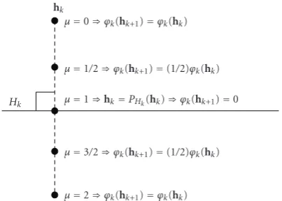
μ=0⇒ϕk(hk+1)=ϕk(hk)

μ=1/2⇒ϕk(hk+1)=(1/2)ϕk(hk) μ=1⇒hk=PHk(hk)⇒ϕk(hk+1)=0

μ=3/2⇒ϕk(hk+1)=(1/2)ϕk(hk)

μ=2⇒ϕk(hk+1)=ϕk(hk) Hk

hk

Figure 1: Reduction of the metric distance function ϕk(x) := d(x,Hk) by the relaxed projection.

Here,uk:=[uk,uk−1,. . .,uk−N+1]T ∈RNis the input vector at time kwith (uk)k∈Nbeing the observable input process,

h∗ ∈ RN _{the unknown system, (n}

k)k∈Nthe noise process,

and (dk)k∈Nthe observable output process. In the parameter

estimation problem, for instance, the goal is to estimate h∗. Given an initialh0 ∈ RN, the NLMS algorithm [4,5] generates the vector sequence (hk)k∈Nrecursively as follows:

hk+1:=hk−μek(hk)

uk22

uk (3)

=hk+μ

PHk(hk)−hk

, k∈N, (4) whereμ ∈ [0, 2] is the step size (In the presence of noise,

μ >1 would never be used in practice due to its unacceptable misadjustment without increasing the speed of convergence.) and

ek(h) := uk,h2−dk, h∈RN, k∈N, (5)

Hk:=

h∈RN_:e k(h)=0

, k∈N. (6) The right side of (4) is called the relaxed projectiondue to the presence ofμ, and it is illustrated inFigure 1. We see that for anyμ∈(0, 2) the update of NLMS decreases the value of the metric distance function:

ϕk(x) :=d(x,Hk) :=min a∈Hk

x−a2, x∈RN, k∈N. (7)

Figure 2 illustrates several steps of NLMS for μ = 1. In noiseless case, it is readily verified thatϕk(h∗)=d(h∗,Hk)=

0, for all k ∈ N, implying that (i) h∗ ∈ k∈NHk and

(ii) hk+1−h∗2 ≤ hk−h∗2, for all k ∈ N, due to the Pythagorean theorem. The figure suggests that (hk)k∈N

would converge toh∗; namely, it would minimize (ϕk)k∈N

asymptotically. In noisy case, the properties (i) and (ii) shown above are not guaranteed, and NLMS can only compute an approximate solution. APA [6,7] can be viewed in a similar way [10]. The APSM presented below is an extension of NLMS and APA.

Hk+2

Hk+1

Hk hk+3

hk+2

hk+1

h∗(noiseless case)

hk

Figure 2: NLMS minimizes the sequence of the metric distance functionsϕk(x) := d(x,Hk) asymptotically under certain condi-tions.

a sequence of functions is a natural formulation in the adaptive filtering. The task we consider now is asymptotic minimization of a sequence of (general) continuous convex functions (ϕk)k∈N, ϕk : RN → [0,∞), over a possible

constraint set (∅=/ )C ⊂RN_{, which is assumed to be closed}

and convex. In [2], it has been proven that APSM achieves this task under certain mild conditions by generating a sequence (hk)k∈N ⊂ RN (for an initial vector h0 ∈ RN) recursively by

hk+1:=PC

hk+λk

Tsp(ϕk)(hk)−hk , k∈N, (8)

whereλk∈[0, 2],k∈N, andTsp(ϕk)denotes the subgradient

projection relative toϕk(seeAppendix A). APSM reproduces

NLMS by letting C := RN _{and ϕ}

k(x) := d(x,Hk), x ∈

RN_{, k ∈ N, with the standard inner product. A useful}

generalization has been presented in [3]; this makes it possible to take into account multiple convex constraints in the parameter space [3] and also such constraints in multiple domains [43,44].

3. Variable-Metric Extension of APSM

We extend APSM such that it encompasses the family of adaptive variable-metric projection algorithms, which have remarkable advantages in performance over their constant-metric counterparts. We start with a simplified version of the variable-metric APSM (V-APSM) and show that it includes TDAF, LNAF/QNAF, PAF, and KPAF as its particular examples. We then present the V-APSM that can deal with a convex constraint (the reader who has no need to consider any constraint may skipSection 3.3).

3.1. Variable-Metric Adaptive Projected Subgradient Method without Constraint. We present the simplified V-APSM which does not take into account any constraint (The full version will be presented inSection 3.3). Let (RN×N _)G

k

0, k ∈ N; we express by A 0 that a matrix A is symmetric and positive definite. Define the inner product and its induced norm, respectively, asx,y_Gk:=xT_G

ky, for

all (x,y)∈RN_×RN_{, andx} Gk:=

x,xGk, for allx∈R

N_.

For convenience, we regard Gk as a metric. Recalling the

definition, the subgradient projection depends on the inner

product (and the norm), thus depending on the metricGk

(see (A.3) and (A.4) inAppendix A). We therefore specify the metricGkemployed in the subgradient projection byTsp((Gkϕ)k).

The simplified variable-metric APSM is given as follows.

Scheme 1 (Variable-metric APSM without constraint). Let

ϕk:RN → [0,∞),k ∈N, be continuous convex functions.

Given an initial vectorh0∈RN, generate (hk)k∈N⊂RN by

hk+1:=hk+λk

T(Gk)

sp(ϕk)(hk)−hk , k∈N, (9)

whereλk∈[0, 2], for allk∈N.

Recalling the linear system model presented in

Section 2.1, a simple example of Scheme 1 is given as follows.

Example 1 (Adaptive variable-metric projection algorithms). An application ofScheme 1to

ϕk(x) :=dGk(x,Hk) :=min

a∈Hk

x−aGk, x∈R

N_,k∈N

(10)

yields

hk+1:=hk+λk

P(Gk)

Hk (hk)−hk

=hk−λk ek

(hk)

uT_kG−1

k uk

G−_k1uk, k∈N.

(11)

Equation (11) is obtained by noting that the normal vector of Hk with respect to the Gk-metric is Gk−1uk because

Hk = {h ∈ RN :Gk−1uk,hGk = dk}. More sophisticated

algorithms thanExample 1can be derived by following the way in [2, 37]. To keep this work as simple as possible for better accessibility, such sophisticated algorithms will be investigated elsewhere.

3.2. Examples of the Metric Design. The TDAF, LNAF/QNAF, PAF, and KPAF algorithms have the common form of (11) with individual design of Gk; interesting relations among

TDAF, PAF, and KPAF are given in [34] based on the so-called error surface analysis. The Gk-design in each of the

algorithms is given as follows.

(1) Let V ∈ RN×N _{be a prespecified transformation}

matrix such as the discrete cosine transform (DCT) and discrete Fourier transform (DFT). Givens(0i)>0,

i = 1, 2,. . .,N, defines(ki+1) := γs (i)

k + (u

(i)

k )

2 , where

γ ∈ (0, 1) and [u(1)k ,u

(2)

k ,. . .,u

(N)

k ]

T

:= Vuk is the

transform-domain input vector. Then,Gkfor TDAF

[19,20] is given as follows: Gk:=VTdiag

s(1)k ,s

(2)

k ,. . .,s

(N)

k V. (12)

Here, diag(a) denotes the diagonal matrix whose diagonal entries are given by the components of a vectora∈RN_{. This metric is useful for colored input}

(2)Gks for LNAF in [23] and QNAF in [26] are given by

Gk :=Rk,LNandGk:=Rk,QN, respectively, where for some initial matricesR0,LN andR0,QN their inverses are updated as follows:

R−1

k+1,LN:= 1 1−α

⎛ ⎝R−1

k,LN−

R_k−_,LN1 ukuTkR−k,LN1 (1−α)/α+u_kTR−_k,LN1 uk

⎞ ⎠_,

α∈(0, 1),

R−1

k+1,QN:=R−k,QN1 + ⎛

⎝ 1

2uT_kR−_k,QN1 uk

−1

⎞

⎠R−k,QN1 ukuTkR−k,QN1 uT_kR−_k,QN1 uk

.

(13)

The matricesRk,LN andRk,QN well approximate the autocorrelation matrix of the input vectoruk, which

coincides with the Hessian of the mean squared error (MSE) cost function. Therefore, LNAF/QNAF is a stochastic approximation of the Newton method, yielding faster convergence than the LMS-type algo-rithms based on the steepest descent method.

(3) Let hk =: [h(1)k ,h

(2)

k ,. . .,h

(N)

k ]

T

, k ∈ N. Given small constants σ > 0 and δ > 0, define

Lmax

k :=max{δ,|h

(1)

k |,|h

(2)

k |,. . .,|h

(N)

k |} >0,γ

(n)

k :=

max{σLmaxk ,|h

(n)

k |}> 0,n= 1, 2,. . .,N, andα

(n)

k :=

γ(kn)/

N i=1γ

(i)

k , n = 1, 2,. . .,N. Then, Gk for the

PNLMS algorithm [27,28] is as follows:

Gk:=diag−1

α(1)_k ,α(2)_k ,. . .,α(_kN) . (14)

This metric is useful for sparse unknown systems h∗. The improved proportionate NLMS (IPNLMS) algorithm [31] employsγ(ip,n)k:=2[(1−ω)hk1/N+

ω|h(kn)|], ω ∈ [0, 1), forn = 1, 2,. . .,N in place of

γ(kn); · 1denotes the 1norm. IPNLMS is reduced to the standard NLMS algorithm when ω := 0. Another modification has been proposed in, for example, [32].

(4) Let R and p be the estimates of R := E{ukuTk}

and p := E{ukdk}. Also let Q ∈ RN×N be a

matrix obtained by orthonormalizing (from left to right) the Krylov matrix [p, Rp,. . .,RN−1_{p]. Define} [h(1)k ,h

(2)

k ,. . .,h

(N)

k ]

T

:= QT_h

k, k ∈ N. Given a

proportionality factorω∈[0, 1) and a small constant

ε >0, define

βk(n):=

1−ω N +ω

h(kn)

N i=1h(

i)

k +ε

>0,

n=1, 2,. . .,N, k∈N.

(15)

Then,Gkfor KPNLMS [34] is given as follows:

Gk:=Qdiag−1

βk(1),β

(2)

k ,. . .,β

(N)

k QT. (16)

This metric is useful even for dispersive unknown systemsh∗, asQT _{sparsifies it. If the input signal is}

highly colored and the eigenvalues of its autocorrela-tion matrix are notclustered, then this metric is used in combination with the metric of TDAF (see [34]). We mention that this is not exactly the one proposed in [34]. The transformation QT _{makes the optimal}

filter into a special sparse system of which only a few first components would have large magnitude and the rest is nearly zero. This information (which is much more than only that the system is sparse) is exploited to reduce the computational complexity.

Finally, we present below the full version of V-APSM, which is an extension ofScheme 1for dealing with a convex constraint.

3.3. The Variable-Metric Adaptive Projected Subgradient Method—A Treatment of Convex Constraint. We generalize

Scheme 1slightly so as to deal with a constraint setK⊂RN_,

which is assumed to be closed and convex. Given a mapping

T : RN _{→ R}N_{, Fix(T) := {x ∈ R}N _{: T(x) = x}is called}

the fixed point set ofT. The operatorP(Gk)

K ,k ∈ N, which denotes the metric projection ontoKwith respect to theGk

-metric, is 1-attracting nonexpansive(with respect to theGk

-metric) with Fix(P(Gk)

K )=K, for allk∈N(seeAppendix B). It holds moreover thatP(Gk)

K (x) ∈ Kfor anyx ∈ RN. For generality, we letTk :RN → RN,k∈N, be anη-attracting

nonexpansive mapping (η >0) with respect to theGk-metric

satisfying

Tk(x)∈K=Fix(Tk), ∀k∈N,∀x∈RN. (17)

The full version of V-APSM is then given as follows.

Scheme 2 (The Variable-metric APSM). Let ϕk : RN →

[0,∞), k ∈ N, be continuous convex functions. Given an initial vectorh0∈RN, generate (hk)k∈N⊂RN by

hk+1:=Tk

hk+λk

T(Gk)

sp(ϕk)(hk)−hk

, k∈N, (18)

whereλk∈[0, 2], for allk∈N.

Scheme 2 is reduced to Scheme 1 by letting Tk := I

(K = RN_{), for all k ∈ N, where I denotes the identity}

mapping. The form given in (18) was originally presented in [37] without any consideration of the convergence issue. Moreover, a partial convergence analysis for Tk := I was

presented in [45] with no proof. In the following section, we present a more advanced analysis for Scheme 2with a rigorous proof.

4. A Deterministic Analysis

4.1. Monotone Approximation in the Variable-Metric Sense. We start with the following assumption.

Assumption 1. (a) (Assumption in [2]). There existsK0∈N s.t.

ϕ∗_k :=min

x∈Kϕk(x)=0, ∀k≥K0, Ω:=

k≥K0

Ωk= ∅/ ,

(19)

where

Ωk:=

x∈K:ϕk(x)=ϕ∗k

, k∈N. (20)

(b) There existε1,ε2 > 0 s.t.λk ∈ [ε1, 2−ε2] ⊂ (0, 2),

k≥K0.

The following fact is readily verified.

Fact 1. UnderAssumption 1(a), the following statements are equivalent (fork≥K0):

(a)hk∈Ωk,

(b)hk+1=hk,

(c)ϕk(hk)=0,

(d)0∈∂Gkϕk(hk).

V-APSM enjoys a sort of monotone approximation in the Gk-metric sense as follows.

Proposition 1. Let (hk)k∈N be the vectors generated by

Scheme 2. UnderAssumption 1, for anyz∗_k ∈Ωk,

hk−z∗k

2

Gk−

hk+1−z∗k

2

Gk≥ε1ε2

ϕ2k(hk)

ϕk(hk)

2

Gk

(∀k≥K0 s.t.hk∈/ Ωk),

(21)

hk−z∗k

2

Gk−

hk+1−z∗k

2

Gk

≥ ηε2

ε2+ (2−ε2)η

hk−hk+1G2k, ∀k≥K0.

(22)

Proof . SeeAppendix C.

Proposition 1will be used to prove the theorem in the following.

4.2. Analysis under Small Metric-Fluctuations. To prove the deterministic convergence, we need the property ofmonotone approximation in a certain “constant-metric” sense [2]. Unfortunately, this property is not ensured automatically for the adaptive variable-metric projection algorithm unlike the constant-metric one. Indeed, as described inProposition 1, themonotone approximationis only ensuredin theGk-metric

sense at each iteration; this is because the strongly attracting nonexpansivity ofTk and the subgradient projectionTsp((Gkϕ)k)

are both dependent onGk. Therefore, considerably different

metrics may result in totally different directions of update, suggesting that under large metric-fluctuations it would be impossible to ensure the monotone approximation in the “constant-metric” sense. Small metric-fluctuations is thus the key assumption to be made for the analysis.

Given any matrixA∈RN×N_{, its spectral norm is defined}

by A2 := supx∈RNAx2/x2 [46]. Given A 0, let

σmin

A >0 andσAmax >0 denote its minimum and maximum

eigenvalues, respectively; in this case A2 = σAmax. We

introduce the following assumptions.

Assumption 2. (a) Boundedness of the eigenvalues of Gk.

There existδmin,δmax∈(0,∞) s.t.δmin< σGmink ≤σ

max

Gk < δmax,

for allk∈N.

(b) Small metric-fluctuations. There exist (RN×N _)G

0,K1 ≥K0,τ >0, and a closed convex setΓ⊆Ωs.t.Ek :=

Gk−Gsatisfies

hk+1+hk−2z∗2Ek2

hk+1−hk2 <

ε1ε2σGminδmin2 (2−ε2)2σGmaxδmax

−τ

(∀k≥K1s.t.hk∈/Ωk), ∀z∗∈Γ.

(23)

We now reach the convergence theorem.

Theorem 1. Let (hk)k∈N be generated by Scheme 2. Under Assumptions1and2, the following holds.

(a)Monotone approximation in the constant-metric sense. For anyz∗∈Γ,

_hk−z∗2

G−hk+1−z∗2G

≥(2−ε2)2σGmax

δ2 min

τ ϕ

2

k(hk)

ϕk(hk)

2

G

(∀k≥K1s.t.hk∈/Ωk)

(24) hk−z∗2G−hk+1−z∗2G

≥ τ

σmax

G

hk−hk+12G, ∀k≥K1.

(25)

(b)Asymptotic minimization. Assume that(ϕk(hk))k∈Nis bounded. Then,

lim

k→ ∞ϕk(hk)=0. (26)

(c) Convergence to an asymptotically optimal point. Assume that Γ has a relative interior with respect to a hyperplane Π ⊂ RN_{; that is, there exists h ∈ Π∩Γ s.t.}

{x ∈Π :x−h< εr.i.} ⊂Γfor someεr.i. >0. (The norm

· can be arbitrary due to the norm equivalency for finite-dimensional vector spaces.) Then,(hk)k∈Nconverges to a point

h∈K. In addition, under the assumption inTheorem 1(b),

lim

k→ ∞ϕk

h =0 (27)

provided that there exists bounded(ϕk(h))k∈Nwhereϕk(h) ∈

(d)Characterization of the limit point. Assume the exis-tence of some interior point h of Ω. In this case, under the assumptions in (c), if for allε >0, for allr >0,∃δ >0s.t.

inf

d(hk,lev≤0ϕk)≥ε,

h−hk≤r,

k≥K1

ϕk(hk)≥δ,

(28)

then h ∈ lim infk→ ∞Ωk, where lim infk→ ∞Ωk :=

_∞

k=0

n≥kΩn and the overline denotes the closure (see Appendix Afor the definition oflev≤0ϕk). Note that the metric

for · andd(·,·)is arbitrary. Proof. SeeAppendix D.

We conclude this section by giving some remarks on the assumptions and the theorem.

Remark 1 (On Assumption 1). (a) Assumption 1(a) is required even for the simple NLMS algorithm [2].

(b)Assumption 1(b) is natural because the step size is usually controlled so as not to become too large nor small for obtaining reasonable performance.

Remark 2 (On Assumption 2). (a) In the existing algo-rithms mentioned in Example 1, the eigenvalues of Gk

are controllable directly and usually bounded. Therefore,

Assumption 2(a) is natural.

(b)Assumption 2(b) implies that the metric-fluctuations

Ek2should be sufficiently small to satisfy (23). We mention that the constant metric (i.e., Gk := G 0, for all

k ∈ N, thus Ek2 = 0) surely satisfies (23): note that hk+1−hk2=/0 by Fact 1. In the algorithms presented in

Example 1, the fluctuations ofGk tend to become small as

the filter adaptation proceeds. If in particular a constant step sizeλk :=λ ∈(0, 2), for allk ∈N, is used, we haveε1 =λ andε2=2−λand thus (23) becomes

hk+1+hk−2z∗2Ek2

hk+1−hk2

<

2

λ−1

σGminδmin2

σmax

G δmax −

τ. (29)

This implies that the lower the value ofλis, the larger amount of metric-fluctuations would be acceptable in the adaptation. InSection 5, it will be shown that the use of smallλmakes the algorithm relatively insensitive to large metric-fluctuations. Finally, we mention that multiplication ofGk by any scalar

ξ >0 does not affect the assumption, because (i)σmin

G ,σGmax,

δmin,δmax, andEk2in (23) are equally scaled, and (ii) the update equation (23) is unchanged (asϕ_k(x) is scaled by 1/ξ

by the definition of subgradient).

Remark 3 (On Theorem 1). (a) Theorem 1(a) ensures the monotone approximation in the “constant”G-metric sense; that is, hk+1−z∗G ≤ hk−z∗G for any z∗ ∈ Γ.

This remarkable property is important for stability of the algorithm.

(b)Theorem 1(b) tells us that the variable-metric adap-tive filtering algorithm in (11) asymptotically minimizes the sequence of the metric distance functions ϕk(x) =

dGk(x,Hk), k ∈ N. This intuitively means that the output

error ek(hk) diminishes, since Hk is the zero output-error

hyperplane. Note however that this does not imply the convergence of the sequence (hk)k∈N(seeRemark 3(c)). The

condition of boundedness is automatically satisfied for the metric distance functions [2].

(c) Theorem 1(c) ensures the convergence of the sequence (hk)k∈N to a point h ∈ K. An example that the

NLMS algorithm does not converge without the assumption in Theorem 1(c) is given in [2]. Theorem 1(c) also tells us that the limit point h minimizes the function sequence

ϕk asymptotically; that is, the limit point is asymptotically

optimal. In the special case wherenk = 0 (for allk ∈ N)

and the autocorrelation matrix of uk is nonsingular,h∗ is

the unique point that makesϕk(h∗)=0 for allk∈N. The

condition of boundedness is automatically satisfied for the metric distance functions [2].

(d) From Theorem 1(c), we can expect that the limit pointhshould be characterized by means of the intersection of Ωks, because Ωk is the set of minimizers of ϕk on K.

This intuition is verified byTheorem 1(d), which provides an explicit characterization of h. The condition in (28) is automatically satisfied for the metric distance functions [2].

5. Numerical Examples

We first show that V-APSM outperforms its constant-metric (or Euclidean-metric) counterpart with the design of Gk

presented in Section 3.2. We then examine the impacts of metric-fluctuations on the performance of adaptive filter by taking PAF as an analogy; recall here that metric-fluctuations were the key in the analysis. We finally consider the case of nonstationary inputs and present numerical studies on the properties of the monotone approximation and the convergence to an asymptotically optimal point (see

Theorem 1).

5.1. Variable Metric versus Constant Euclidean Metric. First, we compare TDAF [19,20] and PAF (specifically, IPNLMS) [31] with their constant-metric counterpart, that is, NLMS. We consider a sparse unknown systemh∗ ∈ RN _depicted

in Figure 3(a) with N = 256. The input is the colored signal called USASI and the noise is white Gaussian with the signal-to-noise ratio (SNR) 30 dB, where SNR :=

10 log₁₀(E{z2

k}/E{n2k}) with zk := uk,h∗ (The USASI

signal is a wide sense stationary process and is modeled on the autoregressive moving average (ARMA) process characterized by H(z) := (1− z−2_{)/(1 − 1.70223z}−1 ₊ 0.71902z−2_{), z ∈C, whereCdenotes the set of all complex} numbers. In the experiments, the average eigenvalue-spread of the input autocorrelation-matrix was 1.20×106_{.). We set}

λk =0.2, for allk ∈N, for all algorithms. For TDAF, we set

γ = 1−10−3 _{and employ the DCT matrix forV. For PAF} (IPNLMS), we setω=0.5. We use the performance measure of MSE 10 log₁₀(E{e2k}/E{z2k}). The expectation operator is

approximated by an arithmetic average over 300 independent trials. The results are depicted inFigure 3(b).

nonsparse unknown systems h∗ drawn from a normal distribution N(0, 1) randomly at each trial. The other conditions are the same as the first experiment. We setλk =

0.02, for allk ∈N, for KPAF and NLMS, and use the same parameters for KPAF as in [34]. Although the use ofλk=1.0

for QNAF is implicitly suggested in [26], we instead use

λk=0.04 withR−0,Q1N =Ito attain the same steady-state error

as the other algorithms (Idenotes the identity matrix). The results are depicted inFigure 4.

Figures3and4clearly show remarkable advantages of the V-APSM-based algorithms (TDAF, PAF, QNAF, and KPAF) over the constant-metric NLMS. In both experiments, NLMS suffers from slow convergence because of the high correlation of the input signals. The metric designs of TDAF and QNAF accelerate the convergence by reducing the correlation. On the other hand, the metric design of PAF accomplishes it by exploiting the sparse structure ofh∗, and that of KPAF does it by sparsifying the nonsparseh∗.

5.2. Impacts of Metric-Fluctuations on the MSE Performance. We examine the impacts of metric-fluctuations on the MSE performance under the same simulation conditions as the first experiment inSection 5.1. We take IPNLMS because of its convenience in studying the metric-fluctuations as seen below. The metric employed in IPNLMS can be obtained by replacingh∗in

Gideal:=2

1

NI+

diag(|h∗|)

h∗

1 −1

(30)

by its instantaneous estimate hk, where | · | denotes the

elementwise absolute-value operator. We can thus interpret that IPNLMS employs an approximation ofGideal. For ease of evaluating the metric-fluctuations Ek2, we employ a test algorithm which employs the metric Gideal with cyclic fluctuations as follows:

G−_k1:=G−_ideal1 + ρ

Ndiag

eι(k)

, k∈N. (31)

Here,ι(k) :=(kmodN) + 1 ∈ {1, 2,. . .,N},k ∈N,ρ≥0 determines the amount of metric-fluctuations, andej ∈RN

is a unit vector with only one nonzero component at the jth position. LettingG:=Gideal, we have

Ek2=

ρgι_ideal(k) 2

N+ρgidealι(k)

∈0,gidealι(k) , ∀k∈N, (32)

where gn

ideal, n ∈ {1, 2,. . .,N}, denotes the nth diagonal element of Gideal. It is seen that (i) for a givenι(k), Ek2 is monotonically increasing in terms ofρ≥0, and (ii) for a givenρ,Ek2is maximized byg

ι(k) ideal=min

N j=1g

j

ideal.

First, we setλk = 0.2, for allk ∈ N, and examine the

performance of the algorithm forρ = 0, 10, 40.Figure 5(a)

depicts the learning curves. Since the test algorithm has the knowledge about Gideal (subject to the fluctuations depending on theρvalue) from the beginning of adaptation, it achieves faster convergence than PAF (and of course than NLMS). There is a fractional difference betweenρ =0 and

ρ = 10, indicating robustness of the algorithm against a moderate amount of metric-fluctuations. The use ofρ=40, on the other hand, causes the increase of steady-state error and the instability at the end. Meanwhile, the good steady-state performance of IPNLMS suggests that the amount of its metric-fluctuations is sufficiently small.

Next, we setλk=0.1, 0.2, 0.4, for allk∈N, and examine

the MSE performance in the steady-state for each value of

ρ∈[0, 50]. For each trial, the MSE values are averaged over 5000 iterations after convergence. The results are depicted in

Figure 5(b). We observe the tendency that the use of smaller

λkmakes the algorithm less sensitive to metric-fluctuations.

This should not be confused with the well-known relations between the step size and steady-state performance in the standard algorithms such as NLMS. Focusing on ρ = 25 inFigure 5(b), the steady-state MSE ofλk = 0.2 is slightly

higher than that of λk = 0.1, while the steady-state MSE

of λk = 0.4 is unacceptably high compared to that of

λk = 0.2. This does not usually happen in the standard

algorithms.The analysis presented in the previous section offers a rigorous theoretical explanation for the phenomena observed in Figure 5. Namely, the larger the metric-fluctuations or the step size, the more easily Assumption 2(b) is violated, resulting in worse performance. Also, the analysis clearly explains that the use of smallerλkallows a larger amount of

metric-fluctuationsEk2[see (29)].

5.3. Performance for Nonstationary Input. In the previous subsection, we changed the amount of metric-fluctuations in a cyclic fashion and studied its impacts on the performance. We finalize our numerical studies by considering more prac-tical situations in whichAssumption 2(b) is easily violated. Specifically, we examine the performance of TDAF and NLMS for nonstationary inputs of female speech sampled at 8 kHz (seeFigure 6(a)). Indeed, TDAF controls its metric to reduce the correlation of inputs, whose statistical properties change dynamically due to the nonstationarity. The metric therefore would tend to fluctuate dynamically by reflecting the change of statistics. For better controllability of the metric-fluctuations, we slightly modify the update of s(ki)

in (12) into s(ki+1) := γs (i)

k + (1−γ)(u

(i)

k )

2

for γ ∈ (0, 1),

i = 1, 2,. . .,N. The amount of metric-fluctuations can be reduced by increasingγup to one. Considering the acoustic echo cancellation problem (e.g., [33]), we assume SNR 20 dB and use the impulse response h∗ ∈ RN _{(N = 1024)}

described in Figure 6(b), which was recorded in a small room.

For all algorithms, we set λk = 0.02. For TDAF,

we set (A) γ = 1 − 10−4_{, (B) γ = 1 − 10}−4.5_{, and} (C) γ = 1 −10−5_{, and were employ the DCT matrix} for V. In noiseless situations, V-APSM enjoys the mono-tone approximation of h∗ and the convergence to the asymptotically optimal pointh∗ under Assumptions1and

2 (see Remark 3). To illustrate how these properties are affected by the violation of the assumptions due mainly to the noise and the input nonstationarity, Figure 6(c) plots the system mismatch 10 log₁₀(hk−h∗22/h∗

2

the monotone approximation in the G-metric sense,G is unavailable and thus we employ the standard Euclidean metric (note that the convergence doesnot depend on the choice of metric). For (B) γ = 1 −10−4.5 _{and (C) γ =} 1−10−5_{, it is seen thath}

kis approachingh∗monotonically.

This implies that the monotone approximation and the convergence toh∗ arenot seriouslyaffected from a practical point of view. For (A)γ=1−10−4_{, on the other hand,h}

kis

approachingh∗but not monotonically. This is because the use ofγ=1−10−4_{makesAssumption 2(b) violated easily due} to the relatively large metric-fluctuations. Nevertheless, the observed nonmonotone approximation of (A)γ=1−10−4 would be acceptable in practice; on its positive side, it yields the great benefit of faster convergence because it reflects the statistics of latest data more than the others.

6. Conclusion

This paper has presented a unified analytic tool named variable-metric adaptive projected subgradient method (V-APSM). The small metric-fluctuations has been the key for the analysis. It has been proven that V-APSM enjoys the invaluable properties of monotone approximation and convergence to an asymptotically optimal point. Numerical examples have demonstrated the remarkable advantages of V-APSM and its robustness against a moderate amount of metric-fluctuations. Also the examples have shown that the use of small step size robustifies the algorithm against a large amount of metric-fluctuations. This phenomenon should be distinguished from the well-known relations between the step size and steady-state performance, and our analysis has offered a rigorous theoretical explanation for the phenomenon. The results give us a useful insight that, in case an adaptive variable-metric projection algorithm suffers from poor steady-state performance, one could either reduce the step size or control the variable-metric such that its fluctuations become smaller. We believe—and it is our future task to prove—that V-APSM serves as a guiding principle to derive effective adaptive filtering algorithms for a wide range of applications.

Appendices

A. Projected Gradient and Projected

Subgradient Methods

Let us start with the definitions of a convex set and a convex function. A setC ⊂ RN _{is said to be convex ifνx+ (1−}

ν)y∈C, for all (x,y)∈C×C, for allν∈(0, 1). A function

ϕ:RN _{→ Ris said to beconvexifϕ(νx+ (1−ν)y)≤νϕ(x) +}

(1−ν)ϕ(y), for all (x,y)∈RN_×RN_{, for allν∈(0, 1).}

A.1. Projected Gradient Method. The projected gradient method [38,39] is an algorithmic solution to the following convexly constrained optimization:

min

h∈Cϕ(h), (A.1)

whereC ⊂ RN _{is a closed convex set andϕ : R}N _{→ R a}

differentiable convex function with its derivativeϕ:RN _→

RN_{beingκ-Lipschitzian: that is, there existsκ >0 s.t.ϕ(x)−}

ϕ(y) ≤ κx−y, for allx,y ∈ RN_{. For an initial vector}

h0∈RNand the step sizeλ∈(0, 2/κ), the projected gradient method generates a sequence (hk)k∈N⊂RNby

hk+1:=PC

hk−λϕ(hk)

, k∈N. (A.2) It is known that the sequence (hk)k∈N converges to an

arbitrary solution to the problem (A.1). If, however, ϕ

is nondifferentiable, how should we do? An answer to this question has been given by Polyak in 1969 [40], which is described below.

A.2. Projected Subgradient Method. For a continuous (but not necessarily differentiable) convex functionϕ:RN _{→ R,}

it has been proven that the so-called projected subgradient method solves the problem (A.1) iteratively under certain conditions. The interested reader is referred to, for example, [3] for its detailed results. We only explain the method itself, as it is helpful to understand APSM.

What is subgradient, and does it always exist? The subgradient is a generalization of gradient, and it always exists for any continuous (possibly nondifferentiable) convex function (To be precise, the subgradient is a generalization of Gˆateaux differential.). In a differentiable case, the gradient

ϕ(y) at an arbitrary point y ∈ RN _{is characterized as the}

unique vector satisfyingx−y,ϕ(y)+ϕ(y)≤ϕ(x), for all x ∈RN_{. In a nondifferentiable case, however, such a vector}

is nonunique in general, and the set of such vectors

∂ϕy

:=a∈RN _{:x−y,a+ϕy≤ϕ(x),∀x∈R}N

/

= ∅

(A.3)

is called subdifferential of ϕ at y ∈ RN_{. Elements of the}

subdifferential∂ϕ(y) are called subgradientsofϕaty. The projected subgradient method is based on sub-gradient projection, which is defined formally as follows (seeFigure 7for its geometric interpretation). Suppose that lev≤0ϕ := {x ∈ RN : ϕ(x) ≤ 0}= ∅/ . Then, the mapping

Tsp(ϕ):RN → RN defined as

Tsp(ϕ):x−→ ⎧ ⎪ ⎪ ⎨ ⎪ ⎪ ⎩

x−ϕ(x)

ϕ_(x)2ϕ(x) ifϕ(x)>0,

x otherwise

(A.4)

is called subgradient projectionrelative toϕ, whereϕ(x)∈

∂ϕ(x), for all x ∈ RN_{. For an initial vector h}

0 ∈ RN, the projected subgradient method generates a sequence (hk)k∈N⊂RN by

hk+1:=PC

hk+λk

Tsp(ϕ)(hk)−hk , k∈N, (A.5)

where λk ∈ [0, 2], k ∈ N. Comparing (A.2) with (A.4)

and (A.5), one can see similarity between the two methods. However, it should be emphasized that ϕ(hk) is (not the

−1 −0.5 0 0.5 1 1.5

A

m

plitude

0 50 100 150 200 250

Samples (a)

−35 −30 −25 −20 −15 −10 −5 0

MSE

(dB)

102 ₁₀3 ₁₀4 ₁₀5

Number of iterations PAF (IPNLMS)

TDAF

NLMS (constant metric)

(b)

Figure3: (a) Sparse impulse response and (b) MSE performance of NLMS, TDAF, and IPNLMS forλk=0.2. SNR=30 dB,N =256, and colored inputs (USASI).

−15 −10 −5 0

MSE

(dB)

102 ₁₀3 ₁₀4

Number of iterations QNAF

KPAF

NLMS (constant metric)

Figure4: MSE performance of NLMS (λk =0.02), QNAF (λk = 0.04), and KPAF (λk =0.02) for nonsparse impulse responses and colored inputs (USASI). SNR=10 dB,N=256.

B. Definitions of Nonexpansive Mappings

(a) A mappingT is said to be nonexpansiveifT(x)−

T(y) ≤ x−y, for all (x,y)∈RN_×RN_{; intuitively,}

T does not expand the distance between any two pointsxandy.

(b) A mappingTis said to be attracting nonexpansiveifT

is nonexpansive with Fix(T)= ∅_/ andT(x)−f2

<

x−f2

, for all (x,f) ∈ [RN _{\Fix(T)]×Fix(T);}

intuitively,Tattracts any exterior pointxto Fix(T).

(c) A mapping T is said to be strongly attracting nonexpansive or η- attracting nonexpansive if T is nonexpansive with Fix(T)= ∅_/ and there existsη >

0 s.t. ηx−T(x)2 _≤

x−f2 ₋

T(x)−f2 ,

for all (x,f) ∈ RN _{× Fix(T). This condition is}

stronger than that of attracting nonexpansivity, because, for all (x,f) ∈ [RN _{\ Fix(T)] ×Fix(T),}

the differencex−f2_{− T(x)−f}2_{is bounded by}

ηx−T(x)2

>0.

A mapping T : RN _{→ R}N _{with Fix(T)= ∅/ is called}

quasi-nonexpansiveifT(x)−T(f) ≤ x−ffor all (x,f)∈

RN _×Fix(T).

C. Proof of

Proposition 1

Due to the nonexpansivity of Tk with respect to the Gk

-metric, (21) is verified by following the proof of [2, Theo-rem 2]. Noticing the property of the subgradient projection Fix(T(Gk)

sp(ϕk))=lev≤0ϕk, we can verify that the mappingTk:=

Tk[I+λk(Tsp((Gkϕ)k)−I)] is (2−λk)η/(2−λk(1−η))-attracting

quasi-nonexpansive with respect toGkwith Fix(Tk)=K∩

lev≤0ϕk = Ωk (cf. [3]). Because ((2−λk)η)/(2−λk(1−

η)) = [1/η+ (λk/(2−λk))]−1 = [1/η+ (2/λk−1)−1] −1

≥

(ηε2)/(ε2+ (2−ε2)η), (22) is verified.

D. Proof of

Theorem 1

Proof of (a). In the case ofhk ∈ Ωk, Fact1suggestshk+1 = hk; thus (25) holds with equality. In the following, we assume

hk∈/Ωk(⇔hk+1=/ hk). For anyx∈RN, we have

xTGkx=

# yT_H

ky

yT_y

$

−35 −30 −25 −20 −15 −10 −5 0 MSE (dB)

102 ₁₀3 ₁₀4 ₁₀5

Number of iterations

Test(ρ=40)

Test(ρ=0, 10)

PAF (IPNLMS) NLMS (constant metric)

(a) −35 −30 −25 −20 −15 −10 −5 0 St ead y-stat e MSE (dB)

0 10 20 30 40 50

ρ

λk=0.2

λk=0.1 λk=0.4

(b)

Figure5: (a) MSE learning curves forλk=0.2 and (b) steady-state MSE values forλk=0.1, 0.2, 0.4. SNR=30 dB,N =256, and colored inputs (USASI).

where y := G1/2_{x and H}

k := G−1/2GkG−1/2 0. By

Assumption 2(a), we obtain

σmax

Hk = Hk2≤

G−1/2

2Gk2 G−1/2

2=

σmax

Gk

σGmin

< δmax σGmin

σmin

Hk

−1

=H−1

k ₂≤G1/2₂G−k1₂G1/2₂=

σGmax

σmin

Gk

<σ

max

G

δmin. (D.2)

By (D.1) and (D.2), it follows that

δmin

σGmax

x2

G<x2Gk<

δmax

σmin

G

x2

G, ∀k≥K1, ∀x∈RN. (D.3)

NotingET

k =Ek, for allk≥K1(becauseGTk =GkandGT =

G), we have, for allz∗∈Γ⊆Ω⊂Ωkand (for allk≥K1s.t. hk∈/ Ωk),

_hk−z∗2

G−hk+1−z∗2G

=hk−z∗G2k−hk+1−z

∗2

Gk

−(hk−z∗)TEk(hk−z∗) + (hk+1−z∗)TEk(hk+1−z∗)

≥ε1ε2

ϕ2

k(hk)

ϕk(hk)

2

Gk

+ (hk+1+hk−2z∗)TEk(hk+1−hk)

≥ ε1ε2σGmin

δmax

ϕ2k(hk)

ϕk(hk)

2

G

−hk+1+hk−2z∗2Ek2

× hk+1−hk2.

(D.4)

The first inequality is verified byProposition 1and the sec-ond one is verified by (D.3), the Cauchy-Schwarz inequality,

and the basic property of induced norms. Here, δmin <

σmin

Gk ≤(x

T_G

kx)/(xTx) implies

hk+1−hk22<(δmin)−1hk+1−hk2Gk

≤(δmin)−1λ2k

ϕ2k(hk)

ϕk(hk)

2

Gk

<(2−ε2)

2

σGmax

δ2 min

ϕ2

k(hk)

ϕk(hk)

2

G

,

(D.5)

where the second inequality is verified by substitutinghk+1=

Tk[hk−λk(ϕk(hk)/ϕk(hk)2Gk)ϕ

k(hk)] andhk=Tk(hk) (⇐

hk∈K=Fix(Tk); see (17)) and noticing the nonexpansivity

of Tk with respect to the Gk-metric. By (D.4), (D.5), and

Assumption 2(b), it follows that, for allz∗ ∈Γ, for allk ≥

K1s.t.hk∈/Ωk,

_hk−z∗2

G−hk+1−z∗2G

≥ #

ε1ε2σGmin

δmax −

hk+1+hk−2z∗2Ek2

hk+1−hk2

(2−ε2)2σGmax

δ2 min

$

× ϕ2k(hk)

ϕk(hk)

2

G

> (2−ε2)

2

σGmax

δ2 min

τ ϕ

2

k(hk)

ϕk(hk)

2

G

(D.6)

which verifies (24). Moreover, from (D.3) and (D.5), it is verified that

ϕ2k(hk)

ϕk(hk)

2

G

> δmin

(2−ε2)2σGmax

hk+1−hk2Gk

> 1

(2−ε2)2 #

δmin

σGmax

$2

hk+1−hk2G.

(D.7)

−0.5 0 0.5

0 1 2 3 4 5 6 7 8 9 10

M

ag

nitude

×104

Samples (a)

−0.4 −0.2 0 0.2 0.4

A

m

plitude

0 200 400 600 800 1000

Samples (b)

−10 −8 −6 −4 −2 0

Sy

st

em

mismat

ch

(dB)

0 2 4 6 8 10

×104

Number of iterations

NLMS (constant metric)

TDAF (C)

TDAF (B)

TDAF (A)

(c)

Figure 6: (a) Speech input signal, (b) recorded room impulse response, and (c) system mismatch performance of NLMS and TDAF forλk = 0.02, SNR= 20 dB, andN = 1024. For TDAF, (A)γ=1−10−4_{, (B)γ=1−10}−4.5_{, and (C)γ=1−10}−5_.

ϕ

ϕ(x)

Tsp(ϕ)(x)

lev≤0ϕ=∅

RN _x∈RN

Figure7: Subgradient projectionTsp(ϕ)(x)∈RN is the projection

ofxonto the separating hyperplane (the thick line), which is the intersection ofRN_{and the tangent plane at (x,ϕ(x))∈R}N_×R.

Proof of (b). From Fact1, for proving limk→ ∞ϕk(hk)=0, it

is sufficient to check the casehk∈/Ωk(⇒ϕk(hk)=/0). In this

case, byTheorem 1(a), _hk−z∗2

G−hk+1−z∗2G

≥(2−ε2)

2

σGmax

δ2 min

τ ϕ

2

k(hk)

ϕk(hk)

2

G

≥0. (D.8)

For anyz∗∈Γ, the nonnegative sequence (hk−z∗G)k≥K1

is monotonically nonincreasing, thus convergent. This implies that

lim

k→ ∞ ϕk(hk)=/0

ϕ2

k(hk)

ϕk(hk)

2

G

=0; _(D.9)

hence the boundedness of (ϕk(hk))k∈N ensures

limk→ ∞ϕk(hk)=0.

Proof of (c). By Theorem 1(a) and [2, Theorem 1], the sequence (hk)k≥K1 converges to a point h ∈ RN. The

closedness ofK(hk, for allk∈N\ {0}) ensuresh∈K.

By the definition of subgradients and Assumption 2(a), we obtain

0≤ϕk

h ≤ϕk(hk)−

%

hk−h, ϕk(h)

&

Gk

≤ϕk(hk) +hk−h

2Gk2 ϕk(h) ₂

< ϕk(hk) +δmaxhk−h

2

ϕk(h)₂.

(D.10)

Hence, noticing (i) Theorem 1(b) under the assumption, (ii) the convergencehk → h, and (iii) the boundedness of

(ϕk(h))k∈N, it follows that limk→ ∞ϕk(h) =0.

Proof of (d). The claim can be verified in the same way as in [2, Theorem 2(d)].

Acknowledgment

The authors would like to thank the anonymous reviewers for their invaluable suggestions which improved particularly the simulation part.

References

[1] I. Yamada, “Adaptive projected subgradient method: a unified view for projection based adaptive algorithms,”The Journal of IEICE, vol. 86, no. 8, pp. 654–658, 2003 (Japanese).

[2] I. Yamada and N. Ogura, “Adaptive projected subgradient method for asymptotic minimization of sequence of nonneg-ative convex functions,” Numerical Functional Analysis and Optimization, vol. 25, no. 7-8, pp. 593–617, 2004.