Volume 2009, Article ID 367465,7pages doi:10.1155/2009/367465
Research Article
A New Mutated Quantum-Behaved Particle Swarm Optimizer for
Digital IIR Filter Design
Wei Fang, Jun Sun, and Wenbo Xu
Centre of Intelligent and High Performance Computing, School of Information Technology, Jiangnan University, no 1800, Lihu Avenue, Wuxi 214122, China
Correspondence should be addressed to Wei Fang,[email protected]
Received 28 July 2009; Accepted 21 November 2009
Recommended by Kutluyil Dogancay
Adaptive infinite impulse response (IIR) filters have shown their worth in a wide range of practical applications. Because the error surface of IIR filters is multimodal in most cases, global optimization techniques are required for avoiding local minima. In this paper, we employ a global optimization algorithm, Quantum-behaved particle swarm optimization (QPSO) that was proposed by us previously, and its mutated version in the design of digital IIR filter. The mechanism in QPSO is based on the quantum behaviour of particles in a potential well and particle swarm optimization (PSO) algorithm. QPSO is characterized by fast convergence, good search ability, and easy implementation. The mutated QPSO (MuQPSO) is proposed in this paper by using a random vector in QPSO to increase the randomness and to enhance the global search ability. Experimental results on three examples show that QPSO and MuQPSO are superior to genetic algorithm (GA), differential evolution (DE) algorithm, and PSO algorithm in quality, convergence speed, and robustness.
Copyright © 2009 Wei Fang et al. This is an open access article distributed under the Creative Commons Attribution License, which permits unrestricted use, distribution, and reproduction in any medium, provided the original work is properly cited.
1. Introduction
Adaptive IIR filters have been proven to be useful in many fields such as channel equation, noise reduction, echo cancelling, and system identification [1,2]. A major problem in adaptive IIR filters design is that their error surface may be usually nonquadratic and multimodal. If this problem is considered, global optimization technique is required to get the global minima in a multimodal error surface. In the recent years, population-based intelligent algorithms and heuristic algorithms, such as genetic algorithm (GA) [3–
6], simulated annealing (SA) algorithm [3, 7], differential evolutionary (DE) [8] algorithm, particle swarm optimiza-tion (PSO) algorithm [9,10], Tabu search (TS) algorithm [11], ant colony optimization (ACO) [12] algorithm, and artificial bee colony algorithm [13], have been proposed and used in the digital IIR filter design. GA has received considerable attention for the digital IIR filter design. How-ever, its disadvantages are lack of good local search ability and premature convergence. The drawback of standard SA algorithm is that it can be very slow and often requires much more number of cost function evaluations to converge to the
Table1: Parameter settings for the competitor algorithms.
GA DE PSO QPSO MuQPSO
Parameter Value Parameter Value Parameter Value Parameter Value Parameter Value Crossover rate 0.8 Scaling factor 0.8 w 0.9 → 0.4∗ α 1 → 0.5∗ α 1→ 0.5∗
Mutation rate 0.2 Combination factor 0.8 c1,c2 2 CR 0.8
Population size 10/30/50 (Examples1,2, and3)
Max. iteration 100/500/100 (Examples1,2, and3)
Data length (N) 500/500/100 (Examples1,2, and3)
∗The sign ofa→brepresents that the parameter value is linearly decreased fromatobaccording to the iteration.
This paper is organized as follows. InSection 2, QPSO is described and MuQPSO is proposed. In Section 3, the problem for digital IIR filter design is formulated and the method of applying QPSO and MuQPSO to the design of IIR filters is presented, and the experimental results are given in this section. A conclusion is given inSection 4.
2. QPSO and Its Mutated Version
2.1. QPSO Algorithm. PSO, proposed by Kennedy and
Eberhart [16] and Shi and Eberhart [17], is a new global search technique. The underlying motivation for the devel-opment of PSO was social behaviour of animals such as bird flocking, fish schooling, and swarm theory. In the PSO algorithm, each particle is represented as a potential solution to a problem in D-dimensional space and is denoted as
Xi = (xi1,. . .,xid. . .,xiD).Each particle remembers its own
previous best position and its velocity along each dimension as Vi = (vi1,. . .,vid,. . .,viD).The velocity and position of
particlei at (t+1)th iteration are updated by the following equations:
vi jt+1=w·vi jt +c1·r1tj·
Pi jt −xi jt
+c2·r2tj
Pt g j−xi jt
, rt
1j,r2tj∼U(0, 1),
xt+1
i j =xti j+vti j+1,
(1)
where c1 andc2 are two positive constants, known as the
cognitive and social coefficients, which control the relative proportion of cognition and social interaction, respectively. VectorPi=(Pi1,. . .,Pi j,. . .,PiD) is the best previous position
(the position giving the best fitness value) of particlei, which is calledpbest. And vectorPg =(Pg1,. . .,Pg j,. . .,PgD) is the
best position discovered by the whole population, which is calledgbest. Parameterwis known as inertia weight and the optimal strategy to control it is to initially set to 0.9 and reduce it linearly to 0.4 [17].
QPSO is inspired by quantum mechanics and fundamen-tal theory of particle swarm. In the QPSO algorithm withM
Table 2: Example 1 with randomly chosen initial positions for system identification.
Number of hits
Global minimum Local minimum
{−0.311,−0.906} {0.114, 0.519}
GA 27 73
DE 92 8
PSO 95 5
QPSO 97 3
MuQPSO 100 0
particles inD-dimensional space, the position of particleiat (t+1)th iteration is updated by
xi jt+1=pti j±α·GPtj−xi jt·ln
1
ut i j
, uti j∼U(0, 1),
(2)
pt
i j=ϕti j·Pi jt +
1−ϕt i j
·Pt
g j, ϕti j∼U(0, 1), (3)
GPt=GP1t,GP2t,. . .,GPtD
=
⎛ ⎝ 1
M M
i=1
Pt i1,
1
M M
i=1
Pt i2,. . .,
1
M M
i=1
Pt iD
⎞
⎠, (4)
where parameter α is called contraction-expansion (CE) coefficient. Pi and Pg have the same meanings as those in
PSO.GPis called Mean Best Position, which is defined as the mean of thepbestpositions of all particles.
Table3: Mean values and standard deviations of the filter coefficients inExample 1(mean of 100 random runs with randomly chosen initial positions).
a b CPU time (s)
GA −0.2630±0.2084 −0.6125±0.5222 7.843
DE −0.2754±0.1164 −0.7926±0.3891 2.780
PSO −0.2892±0.0965 −0.8366±0.3063 2.785
QPSO −0.2919±0.0902 −0.8522±0.2720 2.334
MuQPSO −0.3106±0.0094 −0.9067±0.0034 2.308
2.2. The Mutated QPSO Algorithm. Although QPSO
pos-sesses better global search behaviour than PSO, it may encounter premature convergence [18], a major problem also encountered by GA, PSO, and other evolutionary algorithms in multimodal optimization, which results in great performance loss and suboptimal solutions. In QPSO, although the search space of an individual particle is the whole feasible solution space of the problem throughout the iterations, diversity loss of the whole population is also inevitable due to the collectiveness. From (2), one can see that if |GPj −xi j| is small enough, the search space will
be narrowed and xi j cannot obtain a new position in the
upcoming iterations. The explorative power of particles is lost and the evolution process will stagnate. This case can even occur at an early stage if|GPj−xi j|is zero. In the latter
stage of evolution process, the loss of diversity for|GPj − xi j| is often occurred. To prevent this undesirable trend, a
random vector is constructed according to the difference between two positional coordinates that are rerandomized in the problem space, and the value of the random vector will replace|GPj−xi j|with a certain probabilityCR. Then the
particle’s position is updated by the following equation:
−→
δ =mu xk−mu xs, xi jt+1=pti j±α· − →
δ·ln
1
uti j
,
(5)
wheremu xkandmu xsare two random particles generated
in the problem space. One can see that as the random vector is introduced, the particles may escape from the current position and locate in a new search area.
The variant of QPSO is called MuQPSO. The procedure of MuQPSO is listed as follows.
Step 1. Initialize particles with random position and set the
control parameterCR.
Step 2. For t = 1 to maximum iteration, execute the
following steps.
Step 3. Calculate the mean best position GP among the
particles.
Step 4. For each particle, compute its fitness valuef[xi(t)].If
f[xi(t)]< f[Pi(t)], thenPi(t)=xi(t).
Step 5. SelectgbestpositionPg(t) among particles.
Step 6. Generate a random number, denoted asRN, in the
range of (0 1).
Step 7. IfRN<CRthen update the position according to (2),
(3), (4), else according to (3), (5).
3. Application of QPSO and MuQPSO to
the Design Problem
3.1. Problem Formulation. In general, the basic structure of
an IIR filter is identical to that of the autoregressive moving-average (ARMA) model, whose input-output relation is defined by the following difference equation [2]:
y(k) +
M
i=1
biy(k−i)= L
i=0
aix(k−i), (6)
where x(k) and y(k) are the filter’s input and output, respectively, andM(>=L) is the filter order,aiandbiare the
adjustable coefficients of the model. The transfer function of this IIR filter can be written in the following general form:
H(z)= A(z)
1 +B(z)=
L i=0aiz−i
1 +Mi=1biz−i
. (7)
Then an IIR filter design can be formulated as an optimization problem with the mean square error (MSE) as the cost function
J(w)=Ee2(k)=Ed(k)−y(k)2
, (8)
whered(k) is the filter’s desired response,e(k)=d(k)−y(k) is the filter’s error signal, and the composite weight vector of the filter is defined by concatenating the two sets of coefficients{ai}Li=0 and{bi}Mi=1, according to the formula
=[a0,a1,. . .,aL,b1,. . .,bM]T. (9)
The goal is to minimize MSE (8) by adjusting. In practice, ensemble operation is difficult to realize, and the cost function (8) is usually substituted by the time-averaged cost function
J()= 1 N
N
k=1
e2(k), (10)
Table4: Mean values of the filter coefficients inExample 1(mean of 100 random runs with four fixed positions).
Fixed initial positions
{0.114, 0.519} {0.8, 0} {0.9,−0.9} {0.9, 0.9} CPU time (s)
a b a b a b a b
GA 0.1131 0.5243 −0.0361 0.0526 −0.1697 −0.4768 −0.2630 −0.6125 7.470 PSO 0.1140 0.5190 0.0447 0 0.9000 −0.9000 0.9000 0.9000 2.700 DE 0.1140 0.5190 0.8000 0 0.9000 −0.9000 0.9000 0.9000 2.650 QPSO 0.1140 0.5190 0.8000 0 0.9000 −0.9000 0.9000 0.9000 2.515 MuQPSO −0.3105 −0.9068 −0.3105 −0.9070 −0.3104 −0.9066 −0.3108 −0.9073 2.298
−0.32 −0.3 −0.28 −0.26 −0.24 −0.22 −0.2 −0.18 −0.16
a
20 40 60 80 100
Iterations GA
DE PSO
QPSO MuQPSO Optimal value (a)
−1 −0.9 −0.8 −0.7 −0.6 −0.5 −0.4 −0.3
20 40 60 80 100
b
Iterations GA
DE PSO
QPSO MuQPSO Optimal value (b)
0.2 0.25 0.3 0.35 0.4 0.45
20 40 60 80 100
Iterations
Av
er
ag
ed
co
st
fu
n
ct
io
n
va
lu
e
GA DE PSO
QPSO MuQPSO (c)
0.012 0.014 0.016 0.018 0.02 0.022 0.024
0 100 200 300 400
GA DE PSO
QPSO MuQPSO Iterations
Av
er
ag
ed
co
st
fu
n
ct
io
n
va
lu
e
(a)
0 0.05 0.1 0.15 0.2
20 40 60 80 100
GA DE PSO
QPSO MuQPSO Iteration
Av
er
ag
ed
co
st
fu
n
ct
io
n
va
lu
e
(b)
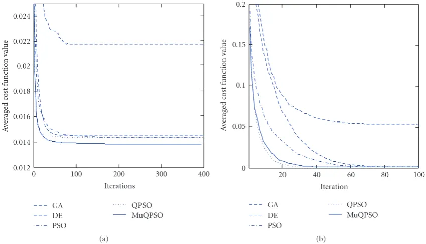
Figure2: Comparison of convergence behaviours for (a)Example 2and (b)Example 3.
In order to apply QPSO and MuQPSO to design the digital IIR filters, the filter coefficients defined in (9) are represented as a particle in QPSO and MuQPSO. The particle is real coded and is treated as a trial solution. The dimension of a particle is equal to the size of the parameter vector
and each dimension of a particle is in correspondence to a filter coefficient. The stability of the filter is guaranteed by constraining the range of the particles’ position [8]. The fitness of a particle is evaluated by its position and the fitness value is calculated using the cost function (10). The lengthN
of the cost function is selected according to the problem.
3.2. Experimental Results. Three examples are used in the
simulation studies. GA, DE, and PSO algorithm are also used for the digital IIR filter design in order to make a per-formance comparison with QPSO and MuQPSO. For each simulation, 100 Monte Carlo simulations are performed. The parameter settings of each example for the competitor algorithms are shown inTable 1.
Example 1(see [3,7,8,11,12]). The unknown plant and the
filter have the following transfer functions:
Hp(z)= 0.05−0.4z
−1
1−1.1314z−1+ 0.25z−2, H(z)=
a
1 +bz−1.
(11)
As the plant is a second-order system and the filter is a first-order IIR filter, local minima problems could be encountered. The system input, x(k), was chosen to be random Gaussian noise with zero mean and unit variance. The error surface has a global minimum at
{a,b} = {−0.311,−0.906}and a local minimum at{a,b} = {0.114, 0.519}.For all the five algorithms, the search space
is (−1, 1). Randomly chosen initial positions and fixed initial positions are considered in the simulation. The fixed initial positions are{0.114, 0.519},{0.8, 0},{0.9,−0.9}, and
{0.9, 0.9}[7].
Table 2 shows the comparison of the number of global and local minimum hits by various algorithms. The results are given by 100 random simulations with randomly chosen initial positions. The table lists that GA is likely to converge to the local minimum. DE, PSO, and QPSO might jump to the global minimum valley with more opportunities and converge to the global minimum, but it also can jump to the local minimum valley and then converge to the local minimum. MuQPSO could converge to the global minimum in all the runs. Tables3and4demonstrate the mean values of filter coefficients along with the standard deviations and the CPU times of each algorithm. From Table 3, one can see that MuQPSO could find the global minimum with the least standard deviations among all the five algorithms. As seen from Table 4, MuQPSO can jump out of any of the settled fixed initial positions and find the global minimum while the other algorithms are all trapped in these fixed initial algorithms.Figure 1presents the coefficients learning curves and convergence behaviours of the five algorithms applied to designExample 1. The results are averaged over 100 random runs with randomly chosen initial positions.
Example 2(see [7,11]). The plant is a third-order system and
filter is a second-order IIR filter with the following transfer functions:
Hp(z)= −0.3 + 0.4z
−1−0.5z−2
1−1.2z−1+ 0.5z−2−0.1z−3,
H(z)= a0+a1z−1
1 +b1z−1+b2z−2.
Table5: Mean values and standard deviations of the filter coefficients inExample 2(mean of 100 random runs with randomly chosen initial positions).
a0 a1 b1 b2 CPU Time (s)
GA −0.3313±0.1092 −0.0586±0.1205 −0.5450±0.3894 −0.2354±0.30342 72.379 DE −0.3909±0.01380 −0.0769±0.0162 −0.2187±0.01683 −0.5796±0.0148 48.453 PSO −0.3912±0.01317 −0.0761±0.0174 −0.2167±0.01944 −0.5792±0.0176 43.408 QPSO −0.3912±0.01197 −0.0768±0.0176 −0.2164±0.01629 −0.5806±0.0133 51.174 MuQPSO −0.3948±0.01345 −0.0742±0.0195 −0.2230±0.0200 −0.5739±0.0155 44.071
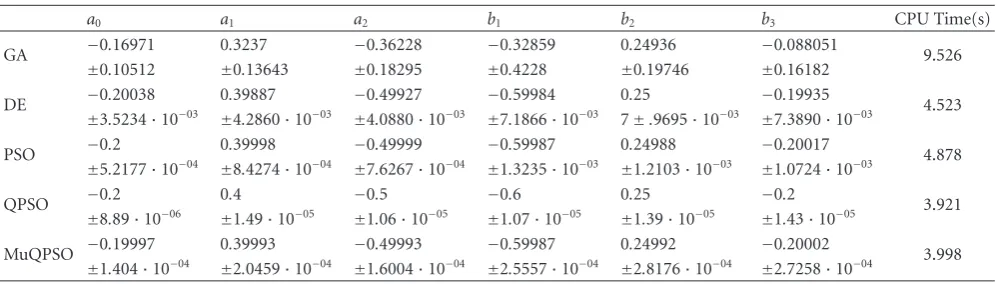
Table6: Mean values and standard deviations of the filter coefficients inExample 3(mean of 100 random runs with randomly chosen initial positions)
a0 a1 a2 b1 b2 b3 CPU Time(s)
GA −0.16971 0.3237 −0.36228 −0.32859 0.24936 −0.088051 9.526
±0.10512 ±0.13643 ±0.18295 ±0.4228 ±0.19746 ±0.16182
DE −0.20038 0.39887 −0.49927 −0.59984 0.25 −0.19935 4.523
±3.5234·10−03 ±4.2860·10−03 ±4.0880·10−03 ±7.1866·10−03 7±.9695·10−03 ±7.3890·10−03
PSO −0.2 0.39998 −0.49999 −0.59987 0.24988 −0.20017 4.878
±5.2177·10−04 ±8.4274·10−04 ±7.6267·10−04 ±1.3235·10−03 ±1.2103·10−03 ±1.0724·10−03
QPSO −0.2 0.4 −0.5 −0.6 0.25 −0.2 3.921
±8.89·10−06 ±1.49·10−05 ±1.06·10−05 ±1.07·10−05 ±1.39·10−05 ±1.43·10−05
MuQPSO −0.19997 0.39993 −0.49993 −0.59987 0.24992 −0.20002 3.998
±1.404·10−04 ±2.0459·10−04 ±1.6004·10−04 ±2.5557·10−04 ±2.8176·10−04 ±2.7258·10−04
The inputx(k), which takes values from (−0.5, 0.5), was a uniformly distributed white sequence, and the SNR=30 dB. Since the reduced order filter is employed for the identifica-tion, the error surface of the cost function is multimodal.
Table 5shows the experimental results by various algo-rithms in Example 2, which gives the mean best values and standard deviations of the filter coefficients. All the results are averaged over 100 random runs with randomly chosen initial positions.Figure 2(a)shows the comparison of convergence behaviours forExample 2. As seen fromTable 5, mean best values produced by PSO, QPSO and MuQPSO are approximate, while QPSO has smaller standard deviation. In
Figure 2(a), one can see that convergence speed of QPSO and MuQPSO is faster than the other three algorithms.
Example 3. The plant and the filter are both third-order
system with the following transfer functions:
Hp(z)= −0.2 + 0.4z
−1−0.5z−2
1−0.6z−1+ 0.25z−2−0.2z−3,
H(z)= a0+a1z−1+a2z−2
1 +b1z−1+b2z−2+b3z−3.
(13)
The inputx(k) was a white Gaussian noise with the mean of zero and unit variance. Since the filter order is equal to that of the system, the error surface is unimodal. The best solution should be located at{−0.2, 0.4,−0.5,−0.6, 0.25,−0.2}.
Table 6shows the mean best values and standard devi-ations of filter coefficients inExample 3averaged over 100 random runs with randomly initial positions. Figure 2(b)
shows the comparison of convergence behaviours for
Example 3 averaged over 100 random runs. As seen from
Table 6, the filter coefficients found by QPSO are exactly located at the best solution and the standard deviation is smaller than that yielded by any other algorithms. QPSO and MuQPSO are the most and the second most robust algorithms among the five ones. FromFigure 2(b), we can see that the convergence speeds of QPSO and MuQPSO are much faster than those of GA, DE, and PSO.
From the above three examples, QPSO and MuQPSO have shown their stronger search abilities both on the multimodal problem and on the unimodal one. QPSO and MuQPSO outperform GA, PSO, and DE in convergence speed, robustness and qualitatively of the final solutions.
4. Conclusions
In this paper, we have introduced the new global optimiza-tion technique, QPSO, and proposed its variaoptimiza-tion, MuQPSO. MuQPSO has enhanced the randomness by modifying the update equation of QPSO. The modified method replaces a part of the update equation with a random vector in a certain probability. QPSO and MuQPSO were both used in the design of digital IIR filters for the purpose of system identification. Experimental results have shown that the performance of QPSO and MuQPSO is superior to GA, DE, and PSO in the digital IIR filter design problem and they will be an efficient tool for this design problem.
Acknowledgment
National Natural Science Foundation of P. R. China (Grant No.60572034, No.60973094), Natural Science Foundation of Jiangsu Province (Grant No. BK2006081), Program for Innovative Research Team of Jiangnan University (Grant No. JNIRT0702), Open foundation of Jiangsu Provincial Key Laboratory of ASIC (Grant No. JSICK0909), and Scientific Research Foundation of Jiangnan University (Grant No. 1055210322090270).
References
[1] J. J. Shynk, “Adaptive IIR filtering,”IEEE ASSP Magazine, vol. 6, no. 2, pp. 4–21, 1989.
[2] S. Haykin,Adaptive Filter Theory, Prentice Hall, Englewood Cliffs, NJ, USA, 4th edition, 2001.
[3] R. Nambiar and P. Mars, “Genetic and annealing approaches to adaptive digital filtering,” inProceedings of the Conference Record of the 62th Asilomar Conference on Signals, Systems and Computers, vol. 2, pp. 871–875, Pacific Grove, Calif, USA, October 1992.
[4] K. S. Tang, K. F. Man, S. Kwong, and Q. He, “Genetic algorithms and their applications,” IEEE Signal Processing Magazine, vol. 13, no. 6, pp. 22–37, 1996.
[5] S. C. Ng, S. H. Leung, C. Y. Chung, A. Luk, and W. H. Lau, “The genetic search approach: a new learning algorithm for adaptive IIR filtering,”IEEE Signal Processing Magazine, vol. 13, no. 6, pp. 38–46, 1996.
[6] Q. Ma and C. F. N. Cowan, “Genetic algorithms applied to the adaptation of IIR filters,”Signal Processing, vol. 48, no. 2, pp. 155–163, 1996.
[7] S. Chen, R. Istepanian, and B. L. Luk, “Digital IIR filter design using adaptive simulated annealing,”Digital Signal Processing, vol. 11, no. 3, pp. 241–251, 2001.
[8] N. Karaboga, “Digital IIR filter design using differential evolution algorithm,” EURASIP Journal on Applied Signal Processing, vol. 2005, no. 8, pp. 1269–1276, 2005.
[9] D. J. Krusienski and W. K. Jenkins, “Adaptive filtering via particle swarm optimization,” inProceedinga of the Conference Record of the Asilomar Conference on Signals, Systems and Computers, vol. 1, pp. 571–575, November 2003.
[10] Y. Gao, Y. Li, and H. Qian, “The design of IIR digital filter based on chaos particle swarm optimization algorithm,” in Proceedings of the 2nd International Conference on Genetic and Evolutionary Computing (WGEC ’08), pp. 303–306, Jingzhou, Hubei, September 2008.
[11] A. Kalinli and N. Karaboga, “A new method for adaptive IIR filter design based on tabu search algorithm,”AEU, vol. 59, no. 2, pp. 111–117, 2005.
[12] N. Karaboga, A. Kalinli, and D. Karaboga, “Designing digital IIR filters using ant colony optimisation algorithm,” Engineer-ing Applications of Artificial Intelligence, vol. 17, no. 3, pp. 301– 309, 2004.
[13] N. Karaboga, “A new design method based on artificial bee colony algorithm for digital IIR filters,”Journal of the Franklin Institute, vol. 346, no. 4, pp. 328–348, 2009.
[14] J. Sun, B. Feng, and W. Xu, “Particle swarm optimization with particles having quantum behavior,” inProceedings of the Congress on Evolutionary Computation (CEC ’04), vol. 1, pp. 325–331, Portland, Ore, USA, June 2004.
[15] J. Sun, W. Xu, and B. Feng, “A global search strategy of quantum-behaved particle swarm optimization,” in Proceed-ings of IEEE Conference on Cybernetics and Intelligent Systems, pp. 111–116, 2004.
[16] J. Kennedy and R. Eberhart, “Particle swarm optimization,” in Proceedings of IEEE International Conference on Neural Networks, vol. 4, pp. 1942–1948, Perth, Australia, November-December 1995.
[17] Y. Shi and R. Eberhart, “Modified particle swarm optimizer,” inProceedings of the IEEE Conference on Evolutionary Com-putation (ICEC’98), pp. 69–73, Anchorage, Alaska, USA, May 1998.