doi:10.1155/2010/942131
Research Article
Evaluation of a Validation Method for MR Imaging-Based Motion
Tracking Using Image Simulation
Kevin M. Moerman,
1Christian M. Kerskens,
2Caitr´ıona Lally,
3Vittoria Flamini,
3and Ciaran K. Simms
11Trinity Centre for Bioengineering, School of Engineering, Parsons Building, Trinity College, Dublin 2, Ireland 2Trinity College Institute of Neuroscience, Trinity College Dublin, Dublin, Ireland
3Mechanical and Manufacturing Engineering, Dublin City University, Dublin, Ireland
Correspondence should be addressed to Kevin M. Moerman,[email protected]
Received 1 May 2009; Accepted 20 July 2009
Academic Editor: Jo˜ao Manuel R. S. Tavares
Copyright © 2010 Kevin M. Moerman et al. This is an open access article distributed under the Creative Commons Attribution License, which permits unrestricted use, distribution, and reproduction in any medium, provided the original work is properly cited.
Magnetic Resonance (MR) imaging-based motion and deformation tracking techniques combined with finite element (FE) analysis are a powerful method for soft tissue constitutive model parameter identification. However, deriving deformation data from MR images is complex and generally requires validation. In this paper a validation method is presented based on a silicone gel phantom containing contrasting spherical markers. Tracking of these markers provides a direct measure of deformation. Validation of in vivo medical imaging techniques is often challenging due to the lack of appropriate reference data and the validation method may lack an appropriate reference. This paper evaluates a validation method using simulated MR image data. This provided an appropriate reference and allowed different error sources to be studied independently and allowed evaluation of the method for various signal-to-noise ratios (SNRs). The geometric bias error was between 0–5.560×10⁻³voxels while the noisy magnitude MR image simulations demonstrated errors under 0.1161 voxels (SNR: 5–35).
1. Introduction
The body responds to mechanical loading on several timescales (e.g., [1,2]), but in vivo measurement of critical parameters such as muscle load, joint reaction force, and tissue stress/strain is usually not possible [3,4]. In contrast, suitably validated computational models can predict all of these parameters, and they are therefore a powerful tool for understanding the musculoskeletal system [4,5] and are in use in diverse applications from impact biomechanics [6,7] to rehabilitation engineering [8,9], surgical simulation [10,11], and soft tissue drug transport [12].
Skeletal muscle tissue in compression is nonlinear elastic, anisotropic, and viscoelastic, and a constitutive model with very good predictive capabilities for in vitro porcine muscle has been proposed [13,14]. However, validating this model for living human tissue presents significant difficulties. Some authors have used indentation tests on skeletal muscle [15, 16], but the tissue was then assumed to be isotropic and
linear in elastic and viscoelastic properties. In contrast, non-invasive imaging methods that allow detailed measurement of human soft tissue motion and deformation (due to known loading conditions) combined with inverse finite element (FE) analysis allow for the evaluation of more complex constitutive models.
The work presented here is part of a study aiming to use indentation tests on the human arm, tagged Magnetic Resonance (MR) imaging and inverse FE analysis to deter-mine the mechanical properties of passive living human skeletal muscle tissue using the constitutive model described in [13,14].
been used to study skin [18], heart [19], and recently also rat skeletal muscle [20] (though a simplified Neo-Hookean model was applied).
The techniques for tracking tissue deformation from (e.g., tagged) MR imaging are complex and require val-idation using an independent measure of deformation. Since physically implanting markers is not feasible and anatomic landmarks are either absent or difficult to track, alternative methods have been employed. Young et al. [21] recorded angular displacement of a silicone gel phantom using tagged MR images and evaluated the results using FE modelling and 2D surface deformation derived from optical tracking of lines painted on the phantom surface. Similarly, Moore et al. [22] used optical tracking of surface lines on a silicone rubber phantom to validate MR-based deformation measures. However simple tensile stretch was applied and only a 2D measure of surface deformation was used. There were also temporal synchronisation issues between the optical and MR image data. In both of the optical validations studies above the error related to the optical tracking method was not quantified. Other authors have used implantable markers. For instance Yeon et al. [23] used implanted crystals and sonomicrometric measurements for validation of tagged MR imaging of the canine heart. However the locations of the crystals were verified manually by mapping with respect to surface cardiac landmarks in the excised heart and matching problems between MR and sonomicrometric measurements occurred. Neu et al. [24,25] evaluated a tagged MR imaging-based deformation tracking technique for cartilage using spherical marker tracking in a silicone soft tissue phantom. However the marker centres were determined by manually fitting a circle to each marker in two orthogonal directions and imaging was performed on excised tissue samples at high resolution (over 32 voxels across marker diameter) using a nonclinical 7.05T scanner.
This paper shows that validation of in vivo medical imaging techniques and image processing algorithms is chal-lenging partially due to the lack of appropriate reference data. Although experimental validation methods using soft tissue MR imaging phantoms can be developed, the data derived from these often suffers uncertainties similar to those present in the target soft tissue. Therefore the validation method itself often lacks an appropriate reference. In this paper a novel technique for the validation of a 3D MR imaging-based motion and deformation tracking technique, applicable to 3D deformation, is presented. The validation method, based on marker tracking, was evaluated (and validated) using simulated magnitude MR image data because this allows full control and knowledge of marker locations and thus provides the final real “gold standard.” It addition this allows for the independent analysis of geometric bias and of method performance across a wide range of realistic noise conditions.
2. Methods
2.1. The Tissue Phantom. The proposed validation
con-figuration is an MR compatible indentor used to apply deformation to a phantom and provides an independent
measure of deformation allowing validation of MR imaging-based motion and deformation tracking. A silicone gel soft tissue phantom was developed to represent deformation modes expected in the human upper arm due to external compression (seeFigure 1), as such the phantom resembles a cylindrical soft tissue region containing a stiffbonelike core. The gel (SYLGARD 527 A&B Dow Corning, MI, USA) has similar MR [26] and mechanical [17] properties to human soft tissue and has been used in numerous MR imaging-based studies on soft tissue biomechanics [21,24,27–34]. Embedded in the gel are contrasting spherical polyoxymethy-lene balls of 3±0.05 mm diameter (The Precision Plastic Ball Co Ltd, Addingham, UK). The lack of signal in the markers in comparison to the high gel signal allows tracking.
2.2. MR Imaging. The type of image data used in the current study is T2 magnitude MR images. Deformation can be measured using marker tracking methods applied to full volume scans taken at each deformation step. A full volume scan was performed on the tissue phantom using a 3T scanner (Philips Achieva 3T, Best, The Netherlands). Cubic 0.5 mm voxels were used and the data was stored using the Digital Imaging and Communication in Medicine (DICOM) format. Figures1(a)and1(b)show an example of an MR image and tagged MR image of a region of the phantom. The voxel intensities of the images are 9 bit unsigned integers with values ranging from 0 to 511. The data was imported into Matlab 7.4 R2007a (The Mathworks Inc., USA) for image processing. The image data was normalised producing an average gel intensity of 0.39, while the marker intensity was zero.
2.3. Marker Tracking Method. To track the movement of
markers from the 3D MR data an image processing algorithm was developed in Matlab (The Mathworks Inc., USA). The centre point of each marker at each time step can be found using 3 main steps: (1)masking,(2)adjacency grouping, and (3)centre point calculation.
(1) Masking. Masking was performed to identify the central voxels for each marker. To reduce computational time the mask was only applied to voxels that qualify (based on intensity threshold) as potentially belonging to a marker. In addition a sparse cross-shaped mask was designed (Figure 2(a)) with just 12 voxels (significantly less than nonsparse cubic or spherical masks which would be around 729 and 250 voxels, resp.). When the mask operates on a voxelvwith image coordinates (i,j,k), the image coordinates of the 12 (surrounding) mask voxels (im,jm,km) can be
defined as ⎛ ⎜ ⎜ ⎝ im jm km ⎞ ⎟ ⎟ ⎠= ⎛ ⎜ ⎜ ⎝
i+ (1,−1, 0, 0, 0, 0, 4,−4, 0, 0, 0, 0) j+ (0, 0, 1,−1, 0, 0, 0, 0, 4,−4, 0, 0) k+ (0, 0, 0, 0, 1,−1, 0, 0, 0, 0, 4,−4) ⎞ ⎟ ⎟ ⎠. (1)
(a) (b) (c)
Figure1: (a) An MR image of a gel region with markers, (b) a tagged MR image region, and (c) the silicone gel soft tissue phantom containing the spherical markers (white balls).
(a) (b) (c)
Figure2: (a) The cross-shaped mask, (b) the adjacency-based grouping process, (c) a 3 mm diameter sphere placed at the calculated marker centre.
(a) (b)
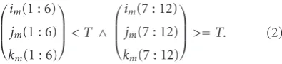
location (i,j,k) is classified as a central marker voxel when all the central cross-mask voxels (see cross-shape inFigure 2(a)) have intensities smaller than the intensity thresholdT and all of the outer voxels (see outer voxels inFigure 2(a)) have intensities higher than or equal to the intensity thresholdT. In other words the following pseudoequation needs to be true:
⎛ ⎜ ⎜ ⎝
im(1 : 6)
jm(1 : 6)
km(1 : 6)
⎞ ⎟ ⎟ ⎠< T ∧
⎛ ⎜ ⎜ ⎝
im(7 : 12)
jm(7 : 12)
km(7 : 12)
⎞ ⎟ ⎟
⎠>=T. (2)
Here all of the first six mask voxels (indicated with 1 : 6), of the mask coordinate collection (im,jm,km),represent the
central cross-elements and the last six (indicated with 7 : 8) represent the outer elements (seeFigure 2(a)). Depending on the marker appearance in the image (see next section) up to 8 central marker voxels match this criterion and were found per marker.
(2) Adjacency Grouping. Calculating the marker centre point using only the central marker voxels identified using masking does not provide an accurate centre point determination (accurate to within a voxel at best) and is sensitive to marker appearance. The more voxels that are included (e.g., all) the better. To find and group voxels deemed to belong to the same marker a grouping algorithm was used. The central marker voxels found using masking were used as starting points to group objects using adjacency analysis. The adjacency grouping is a stepwise process. Adjacency coordinate groups (ACGs) are created for all the voxels found using masking. The process starts with one of the voxels found using maskingvand is assigned to be part of marker groupM. The ACG for this voxelvwith coordinates (i,j,k) is defined as
⎛ ⎜ ⎜ ⎝ if jf kf ⎞ ⎟ ⎟ ⎠= ⎛ ⎜ ⎜ ⎝
i+ (1,−1, 0, 0, 0, 0) j+ (0, 0, 1,−1, 0, 0) k+ (0, 0, 0, 0, 1,−1) ⎞ ⎟ ⎟
⎠. (3)
The ACG contains all the directly adjacent voxels of the voxelv(its direct upper, lower, front, back, left, and right neighbours). Any voxelvwith coordinates (i,j,k) is added to the marker groupM when its intensity is lower thanT and its coordinates are found within one of the ACGs of the markerM. When a voxel is added to the marker groupMits ACG is added to the set of ACGs belonging toM and this process is repeated. Voxels are added to a marker group until the group is no longer growing.
Figure 2(b)shows how, starting with one central voxel, the surrounding low intensity voxels within the coordinate group (if,jf,kf) are added and when this is repeated all
voxels representing the marker are grouped. After grouping, the dimensions and number of voxels of the object were compared to what is expected for normal markers (e.g., a diameter of under 6 voxels and consisting of under 250 voxels) to filter out possible objects other than markers.
(3) Centre Point Calculation. The centre point for each marker group was determined using weighted averaging. The centre coordinates (IM,JM,KM) of a markerMcomposed of
Nvoxels is defined as
(IM JM KM)=
N a=1waia
N a=1wa
N a=1waja
N a=1wa
N a=1waka
N a=1wa
.
(4)
Here average i, j, andk represent the coordinates of each of the voxels in the marker group. Since those voxels with intensities close to zero are more likely to belong to a marker than voxels with intensities close to the gel intensity, the weightwafor a voxel with intensityzawas defined as:
wa=
1−zTa
, withwa=0 ifza> T. (5)
HereT represents a threshold which for a noiseless image could be set equal to the gel intensity (the weightwa then
represents the volume fraction of marker material present in the voxel). The condition is added that whenzais larger than Tthe weightwa=0.
2.4. Evaluation of Marker Tracking Method Using Simulated
Magnitude MR Image Data. The marker tracking method
was evaluated using simulated magnitude MR image data because this allows full control and knowledge of marker locations and thus provides the final real “gold standard.” The simulated data also allow one to isolate and study errors from different sources. The marker tracking method was evaluated using algorithms developed in Matlab (The Mathworks Inc., USA) and involves the following steps: (1)simulation of a noiseless image and analysis of geometric bias, and (2) simulation of noisy magnitude MR data and analysis of the noise effects. The final noisy image data allows one to evaluate the performance of the method under varying noise conditions while the noiseless image allows for evaluation of the geometric bias implicit in the method.
(a)
1
1
2 5
4
3 2
3
4 5
(b)
Figure4: (a) A marker sphere showing OCV. (b) An OCV showing the tetrahedron in which the appearance of markers varies uniquely. The most symmetric appearances are 1 mid voxel, 2 mid face, 3 mid edge, and 4 voxel corner. Appearance 5 is in the middle of the tetrahedron and shows the resulting asymmetric appearance.
the corresponding volume fraction image at the averaged acquisition resolution (cubic 0.5 mm voxels). By multiplying the obtained volume fraction image with the appropriate gel intensity (average normalised intensity 0.39) a noiseless simulated image is obtained.
The appearance inFigure 3(b)is symmetric because the marker centre point coincides with a voxel corner. However the appearance of objects in images varies depending on their location due to averaging across the discrete elements, in this case voxels, which leads to a geometric bias affecting the marker tracking method. Figure 4(a) shows a marker
(a)
0 0.05 0.1 0.15 0.2 0.25 0.3 0.35
(b)
Figure5: (a) A 3D plot representing the full OCV showing the expected type of geometric bias pattern, and (b) a 2D equivalent.
0.1 0.2 0.3 0.4 0.5 0.6
6
4
2
0 0
0.1 0.2 0.3 P
M
A 0.4
0.5 0.6
0
2 4
6 8
10 12
Figure6: The Rician PDF at variousA/σgratios (0–6). WhenA/σg =0 the Rician PDF reduces to the Rayleigh distribution (blue dots)
however asA/σgincreases to overA/σ >2 the Rician PDF behaves approximately Gaussian (red dots atA/σ=6).
obtainable through varying location within the OCV (e.g., each voxel corner produces the same appearance while mid-edge appearances can be obtained through rotation and mirroring). Thus when the spherical markers (or any other symmetric shape) are averaged across a cubic voxel matrix the appearance varies uniquely within the blue tetrahedron shown inFigure 4(b). All other appearances can be obtained by rotation and mirroring of the appearances in this tetrahedron. Appearances 1–4 are the most symmetric appearances obtainable. Other appearances however can be asymmetric such as case 5 which is obtained when the marker centre coincides with the centre of the tetrahedron. Since the centre point calculation in the marker tracking method is based on an average of marker voxel coordinates, it is
sensitive to symmetry of the marker appearance and as such the error is also related to asymmetry.
It was hypothesised that since OCV points 1–4 inFigure 4 produce symmetric appearances the error here is low and that locations furthest away from these symmetries produce the worst error. If this hypothesis is true the error would follow a pattern similar to that shown inFigure 5(a distance plot from the grid defined by the corner, mid-edge, and middle points) and assuming that each point has the same symmetry “weight,” the worst error should occur in the middle of the longest edge of the tetrahedron.
in the appearances as discussed above, simulations were performed in 1 octant of the OCV only using a grid of points. For visualisation purposes the results were then mirrored to obtain bias measures across the full OCV (similar to Figure 5(a)) producing a 19×19×19 grid. A finer grid was then applied around the maximum bias to closely approximate the location of the real maximum bias. This process was repeated until the found maximum no longer varied significantly.
(2) Simulation of Noisy Magnitude MR Data and Analysis of the Noise Effects. Noise is present in all real MR images, and the performance of the marker tracking method needs to be evaluated in the presence of appropriate noise in the simulated image. During MR imaging, signal is acquired in the frequency domain using receiver coils. To move to the image domain the signal can be sampled at discrete locations and reconstructed using inverse Fourier Transforms. For each reconstructed image voxel in Cartesian space the signal can be expressed as a real signalA(represents the noiseless simulated image) plus a real noise component nR and an imaginary noise componentnI[35]
s=sR+sI=A+nR+inI, withi=√−1. (6)
These independent noise components are identically dis-tributed (with zero mean) and their Probability Density Function (PDF) is Gaussian [35–37]. The magnitudemof a signal can be calculated using
m=(A+nR)2+n2I. (7)
The image intensities in magnitude MR images in the presence of noise follow a Rician distribution [35–38] with a PDF [39,40] given by
Pm
m|A,σg
=σm2
g exp
−A2+m2 2σ2 g I0 Am σ2 g H(m), (8)
whereσg represents the standard deviation of the Gaussian noise, H represents the Heaviside step function (ensuring Pm = 0 for m = 0), and I0 is the 0 order modified Bessel function of the first kind. Figure 6shows a surface plot of the Rician PDF for various A/σg (or SNR) ratios (Figure 6was created using σg = 1, the SNR is therefore A/σg =A). When the noise dominates andA/σg approaches
zero the Rician PDF reduces to the Rayleigh PDF [35, 36] (see blue dots in Figure 6). However, when the signal dominates (A/σg > 2 [36]) the Rician distribution behaves
approximately Gaussian (red dots in Figure 6 are for a Gaussian PDF atA/σg =6) [35,36]. With the knowledge that
whenA=0 the Rician PDF reduces to the Rayleigh PDF,σg
can be estimated by analysis of background noise using [38]
σg =
1 2N N
i=1 m2
i. (9)
Using this equation, and analysis of the background of a normalised T2 MR image of the silicone gel phantom, σg
was estimated to be 0.02. Based on the average normalised gel intensity of 0.39 this corresponds to an SNR of 19.5. However, to evaluate the performance of the marker tracking method in the presence of noise, images were simulated at the worst location found by the geometric bias at a SNR of 5 up to 35. Simulations were performed 10 000 times to obtain an estimate of the error distribution at the various SNR levels.
3. Results
The results are presented in two steps: (1) evaluation of the geometric bias in the marker tracking method, and (2) evaluation of the performance on the marker tracking method in the presence of noise.
(1) Evaluation of the Geometric Bias in the Marker Tracking Method. Figure 7(a) shows the geometric bias error in the absence of noise in an Object Central Voxel (OCV). The colour in each element is the error (in units of voxels) of the marker tracking method for each point on the 3D grid.Figure 7(b)shows 2D image slices throughFigure 7(a) showing the best (1, 2) and worst locations (3). Analysis demonstrated that overall the geometric bias of the marker tracking method ranges from 0 to a maximum of 5.560×10⁻³ (with a mean of 3.149 ×10⁻³ and a standard deviation of 7.771×10⁻⁴) voxels. The error is 0 for the symmetric cases (1–4 in Figure 4) while the maximum error occurs in locations where a marker centre point coincides with 1/1.368th or 1/4.329th of a voxel; see, for example, white points in Figure 7(b) (e.g., at [i,j,k] = [0.731, 0.731, 0.731]).
(2) Evaluation of the Performance on the Marker Tracking Method in the Presence of Noise. The performance of the marker tracking method for the noisy magnitude MR image simulations obtained from the 10 000 simulations at each SNR of 5 up to 35 is presented next. As the SNR increases from 5 to 35 the maximum, mean and minimum voxel errors vary according to Figure 8(a). The standard deviation is plotted inFigure 8(b). Although forT=0.26 the maximum stays below 0.1127 in all cases, the method performs better when T is chosen depending on SNR. To illustrate this Figure 9 shows results for the SNR range 15–35 using T=0.32. Using a higherT means that the marker groups are composed of more voxels and thus a more accurate centre point can be calculated. The maximum voxel error forT =
5 10
15
5 10 15 5 10 15
(a)
0.5 1
1.5
0.5 1
1.5 0.5
1 1.5
Slice 2
×10−3
Slice 1
Slice 3
0.5 1.5 2 2.5 3 3.5
1 4 4.5
(b)
Figure7: (a) The OCV showing the error of the marker tracking method, each grid locations tested. (b) Three 2D image slices through the OCV for the best (Slice 1 and 2) and worst locations (Slice 3).
Max Mean Min
0 20 40
0 0.05 0.1 0.15 0.2
SNR
V
oxe
l e
rr
o
r
(a)
0 20 40
SNR 0
0.005 0.01 0.015
Standar
d de
viation
(b)
Figure8: Results for SNR 5 up to 35 usingT=0.26. (a) The maximum (red dotted line), the mean (blue crossed line), and the minimum voxel error plotted against SNR, and (b) the standard deviation plotted against SNR.
Using simulations the error can be minimised for a given SNR by adjusting theTvalue.
4. Discussion
Several MR imaging-based motion tracking algorithms have been proposed in the literature, for example, tagged MR
0.005
15 20 25
SNR
30 35
0.01 0.015 0.02
V
oxe
l e
rr
o
r
Max Mean Min
(a)
15 20 25
SNR
30 35
0.8 0.9 1.1 1.2 1.3
1
Standar
d de
viation
×10−3
(b)
Figure9: Results for SNR 15 up to 35 usingT=0.32. (a) The maximum (red dotted line), the mean (blue crossed line), and the minimum voxel error plotted against SNR, and (b) the standard deviation plotted against SNR.
as for a variety of different Rician distributed noise levels. The noise-free image data allowed analysis of the error related to the geometric bias independently from other error sources.
Therefore the method proved to be robust with geomet-ric bias errors of between 0–5.560×10⁻³voxels and errors due to noise remaining below 0.1127 voxels for all cases simulated with signal-to-noise ratios from 5 to 35. These results were achieved for a global threshold valueT =0.26. However altering the threshold value based on the SNR may result in a significant increase in accuracy. The optimumT value for a certain SNR can be determined using MR data simulations. Using simulations the error can be minimised for a given SNR by adjusting theTvalue.
The method proposed in this paper has two main advantages. The first is that the data used for validation is simulated and therefore can be chosen to have desired levels of noise. This permitted evaluation of the marker tracking method for different levels of noise which has not been done previously. Secondly, since this validation method is based on MR imaging, the marker tracking experiment and the MR imaging-based motion and deformation tracking can all be performed at the same time within the MR scanner.
Although this method has been developed for application to tagged MR imaging on the upper arm, the methods presented here are not limited to this application and can be applied to validate other types of MR imaging-based motion and deformation tracking techniques. Furthermore, these methods are independent of the chosen phantom shape.
5. Conclusion
A novel marker tracking method has been presented and validated using simulated MR image data. The marker tracking method is robust and the maximum geometric bias was 5.560×10⁻³ voxels while the error due to noise remains below 0.1127 voxels for Rician noise distributions with signal-to-noise ratios from 5 up to 35. This appears to be the only marker tracking algorithm suitable for the validation of MR-based motion and deformation tracking of soft tissue which has been validated against a “gold standard.”
Acknowledgment
This work was funded by a Research Frontiers Grant (06/RF/ENMO76) awarded by Science Foundation Ireland.
References
[1] H. Lissner, M. Lebow, and F. Evans, “Experimental studies on the relation between acceleration and intracranial pressure changes in man,”Surgery Gynecology & Obstetrics, vol. 111, pp. 329–338, 1960.
[2] L. M. McNamara and P. J. Prendergast, “Bone remodelling algorithms incorporating both strain and microdamage stim-uli,”Journal of Biomechanics, vol. 40, no. 6, pp. 1381–1391, 2007.
pressure in the isolated rabbit tibialis anterior muscle,”Journal of Biomechanics, vol. 36, no. 4, pp. 505–512, 2003.
[4] A. Erdemir, S. McLean, W. Herzog, and A. J. van den Bogert, “Model-based estimation of muscle forces exerted during movements,”Clinical Biomechanics, vol. 22, no. 2, pp. 131– 154, 2007.
[5] D. Marjoux, D. Baumgartner, C. Deck, and R. Willinger, “Head injury prediction capability of the HIC, HIP, SIMon and ULP criteria,”Accident Analysis & Prevention, vol. 40, no. 3, pp. 1135–1148, 2008.
[6] H. Muggenthaler, K. von Merten, S. Peldschus, et al., “Exper-imental tests for the validation of active numerical human models,”Forensic Science International, vol. 177, no. 2-3, pp. 184–191, 2008.
[7] P. C. Ivancic, S. Ito, and M. M. Panjabi, “Dynamic sagittal flexibility coefficients of the human cervical spine,”Accident Analysis & Prevention, vol. 39, no. 4, pp. 688–695, 2007. [8] E. Linder-Ganz, N. Shabshin, Y. Itzchak, and A. Gefen,
“Assessment of mechanical conditions in sub-dermal tissues during sitting: a combined experimental-MRI and finite element approach,”Journal of Biomechanics, vol. 40, no. 7, pp. 1443–1454, 2007.
[9] E. Linder-Ganz, N. Shabshin, Y. Itzchak, Z. Yizhar, I. Siev-Ner, and A. Gefen, “Strains and stresses in sub-dermal tissues of the buttocks are greater in paraplegics than in healthy during sitting,”Journal of Biomechanics, vol. 41, no. 3, pp. 567–580, 2008.
[10] Y.-J. Lim and S. De, “Real time simulation of nonlinear tissue response in virtual surgery using the point collocation-based method of finite spheres,”Computer Methods in Applied Mechanics and Engineering, vol. 196, no. 31-32, pp. 3011–3024, 2007.
[11] M. A. Audette, V. Hayward, O. Astley, M. Doyon, G. A. McCallister, and K. Chinzei, “A PC-based system architecture for real-time finite element-based tool-specific surgical simu-lation,” inProceedings of the 18th International Congress and Exhibition on Computer Assisted Radiology and Surgery (CARS ’04), vol. 1268 ofInternational Congress Series, pp. 378–383, June 2004.
[12] P. I. Wu and E. R. Edelman, “Structural biomechanics mod-ulate intramuscular distribution of locally delivered drugs,”
Journal of Biomechanics, vol. 41, no. 13, pp. 2884–2891, 2008. [13] M. Van Loocke, C. G. Lyons, and C. K. Simms, “A validated
model of passive muscle in compression,”Journal of Biome-chanics, vol. 39, no. 16, pp. 2999–3009, 2006.
[14] M. Van Loocke, C. G. Lyons, and C. K. Simms, “Viscoelastic properties of passive skeletal muscle in compression: stress-relaxation behaviour and constitutive modelling,”Journal of Biomechanics, vol. 41, no. 7, pp. 1555–1566, 2008.
[15] A. Gefen, N. Gefen, E. Linder-Ganz, and S. S. Margulies, “In vivo muscle stiffening under bone compression promotes deep pressure sores,”Journal of Biomechanical Engineering, vol. 127, no. 3, pp. 512–524, 2005.
[16] A. Palevski, I. Glaich, S. Portnoy, E. Linder-Ganz, and A. Gefen, “Stress relaxation of porcine gluteus muscle subjected to sudden transverse deformation as related to pressure sore modeling,”Journal of Biomechanical Engineering, vol. 128, no. 5, pp. 782–787, 2006.
[17] K. M. Moerman, C. A. Holt, S. L. Evans, and C. K. Simms, “Digital image correlation and finite element modelling as a method to determine mechanical properties of human soft tissue in vivo,”Journal of Biomechanics, vol. 42, no. 8, pp. 1150–1153, 2009.
[18] M. Tada, N. Nagai, H. Yoshida, and T. Maeno, “Iterative FE analysis for non-invaseice material modeling of a fingertip with layered structure,” inProceedings of the Eurohaptics, Paris, France, 2006.
[19] J. C. Walker, M. B. Ratcliffe, P. Zhang, et al., “Magnetic resonance imaging-based finite element stress analysis after linear repair of left ventricular aneurysm,”Journal of Thoracic and Cardiovascular Surgery, vol. 135, no. 5, pp. 1094–1102, 2008.
[20] K. K. Ceelen, A. Stekelenburg, J. L. J. Mulders, et al., “Vali-dation of a numerical model of skeletal muscle compression with MR tagging: a contribution to pressure ulcer research,”
Journal of Biomechanical Engineering, vol. 130, no. 6, Article ID 061015, 8 pages, 2008.
[21] A. A. Young, L. Axel, L. Dougherty, D. K. Bogen, and C. S. Parenteau, “Validation of tagging with MR imaging to estimate material deformation,”Radiology, vol. 188, no. 1, pp. 101–108, 1993.
[22] C. C. Moore, S. B. Reeder, and E. R. McVeigh, “Tagged MR imaging in a deforming phantom: photographic validation,”
Radiology, vol. 190, no. 3, pp. 765–769, 1994.
[23] S. B. Yeon, N. Reichek, B. A. Tallant, et al., “Validation of in vivo myocardial strain measurement by magnetic resonance tagging with sonomicrometry,”Journal of the American College of Cardiology, vol. 38, no. 2, pp. 555–561, 2001.
[24] C. P. Neu, M. L. Hull, and J. H. Walton, “Error optimization of a three-dimensional magnetic resonance imaging tagging-based cartilage deformation technique,”Magnetic Resonance in Medicine, vol. 54, no. 5, pp. 1290–1294, 2005.
[25] C. P. Neu, M. L. Hull, J. H. Walton, and M. H. Buono-core, “Toward an MRI-based method to determine three-dimensional deformations in articular cartilage,” in Proceed-ings of the Summer Bioengineering Conference, Key Biscayne, Fla, USA, 2003.
[26] D. C. Goldstein, H. L. Kundel, M. E. Daube-Witherspoon, L. E. Thibault, and E. J. Goldstein, “A silicone gel phantom suitable for multimodality imaging,”Investigative Radiology, vol. 22, no. 2, pp. 153–157, 1987.
[27] K. F. Augenstein, B. R. Cowan, I. J. LeGrice, P. M. F. Nielsen, and A. A. Young, “Method and apparatus for soft tissue material parameter estimation using tissue tagged magnetic resonance imaging,”Journal of Biomechanical Engineering, vol. 127, no. 1, pp. 148–157, 2005.
[28] T. S. Denney Jr., J. L. Prince, M. J. Lopez, and E. R. McVeigh, “Optimal tag pattern validation using magnetic resonance imaging,” inProceedings of the IEEE International Conference on Image Processing (ICIP ’94), Austin, Tex, USA, 1994. [29] A. S. Fahmy, A. Krieger, and N. F. Osman, “An integrated
system for real-time detection of stiffmasses with a single compression,”IEEE Transactions on Biomedical Engineering, vol. 53, no. 7, pp. 1286–1293, 2006.
[30] D. L. Kraitchman, A. A. Young, C.-N. Chang, and L. Axel, “Semi-automatic tracking of myocardial motion in MR tagged images,”IEEE Transactions on Medical Imaging, vol. 14, no. 3, pp. 422–433, 1995.
[31] N. F. Osman, “Detecting stiffmasses using strain-encoded (SENC) imaging,”Magnetic Resonance in Medicine, vol. 49, no. 3, pp. 605–608, 2003.
[33] B. T. Wyman, Mechanical Evaluation of the Paced Heart Using Tagged Magnetic Resonance Imaging, The Department of Biomedical Engineering, The Johns Hopkins University, Baltimore, Md, USA, 1999.
[34] A. A. Young, D. L. Kraitchman, L. Dougherty, and L. Axel, “Tracking and finite element analysis of stripe deformation in magnetic resonance tagging,”IEEE Transactions on Medical Imaging, vol. 14, no. 3, pp. 413–421, 1995.
[35] R. M. Henkelman, “Measurement of signal intensities in the presence of noise in MR images,”Medical Physics, vol. 12, no. 2, pp. 232–233, 1985.
[36] H. Gudbjartsson and S. Patz, “The Rician distribution of noisy MRI data,”Magnetic Resonance in Medicine, vol. 34, no. 6, pp. 910–914, 1995.
[37] A. C´ardenas-Blanco, C. Tejos, P. Irarrazaval, and I. Cameron, “Noise in magnitude magnetic resonance images,”Concepts in Magnetic Resonance A, vol. 32, no. 6, pp. 409–416, 2008. [38] S. Aja-Fernandez, C. Alberola-Lopez, and C.-F. Westin, “Noise
and signal estimation in magnitude MRI and Rician dis-tributed images: a LMMSE approach,”IEEE Transactions on Image Processing, vol. 17, no. 8, pp. 1383–1398, 2008. [39] S. O. Rice, “Mathematical analysis of random noise,” Bell
Systems Technical Journal, vol. 23, pp. 282–332, 1944. [40] S. O. Rice, “Mathematical analysis of random noise,” Bell
Systems Technical Journal, vol. 24, pp. 46–156, 1945.
[41] L. Axel, A. Montillo, and D. Kim, “Tagged magnetic resonance imaging of the heart: a survey,”Medical Image Analysis, vol. 9, no. 4, pp. 376–393, 2005.