Nonlinear Dynamics of Transition Waves in Multi-Stable Discrete and Continuous Media

(1)

Discrete and Continuous Media

Thesis by

Neel Nadkarni

In Partial Fulfillment of the Requirements for the degree of

Doctor of Philosophy in Aeronautics

CALIFORNIA INSTITUTE OF TECHNOLOGY Pasadena, California

2017

(2)

Neel Nadkarni

ORCID: 0000-0002-4311-2817

(3)

(4)

ACKNOWLEDGEMENTS

First, I would like to sincerely thank my advisors and mentors, Prof. Chiara Daraio and Prof. Dennis Kochmann. I had the wonderful opportunity of working in theoretical and computational research in Dennis’ group at Caltech, during the academic year, and spending my time performing experiments in Chiara’s group at ETH in Switzerland, over the summers. I have been very lucky to have both of them as advisers as they gave me immense intellectual freedom while pursuing my research while providing necessary guidance. Dennis’ exceptional teaching and theoretical expertise, as well as Chiara’s prowess in experimental research and vibrant enthusiasm will always serve as an inspiration to me. They have both been great role models to me, and have provided constant encouragement throughout the course of my graduate studies. I am very grateful to them for shaping me into a better researcher.

I would also like to convey my gratitude to Prof. Rohan Abeyaratne. He has been a wonderful mentor and collaborating with him has helped me develop my theoretical abilities. His deep knowledge in the physics of phase transitions and continuum mechanics has influenced me immensely in my work. I would also like to thank him for inviting me to the workshop that he was co-organizing, at OIST, in Japan, where I had an opportunity to interact with him over an extended period of time, and learn from him.

I would also like to thank Professors Guruswami Ravichandran and Michael Cross for being on my thesis committee. Professor Ravichandran, thank you for all your guidance. I also wish to express my gratitude to all the professors whose courses I took, during my time at Caltech. I am very grateful for support from the NSF grant No. CMMI-1200319 and the Foster and Coco Stanback Space Innovation Fund that made my graduate life at Caltech possible.

(5)

Ramathasan Thevamaran, Mythili Thevamaran, Matthieu Ulrici and Chenzhang Zhou from the Daraio group. Thanks a lot Alex, for all the engaging discussions about life that we had during our Tuesday dinners. Vidya, I had an awesome time sharing an office with you in the last year. Thank you Tom, for accommodating me during my first visit to ETH – I had a great time discussing about European and Indian culture and traditions. Andre, dinners at Jimmy’s complemented with your dry humor will be missed. Thank you for the wonderful trip to Venice, Deva and Mythili – the experience was made a lot richer by your company. Thank you Katie, Miguel, and Marc for organizing hikes in the beautiful terrains of Switzerland. Thank you Maria Chiara, Paul, Jinwoong, Antonio, and Luca for being awesome office-mates during my time at ETH. I would also like to thank my GALCIT friends from first year, Remi Carmigniani, Melanie Delapierre, Heather Duckworth, Altemurcan Kursunlu, Carlos Laguna, Simon Lapointe, Chris Roh, Kevin Rosenberg, Greg Smetana, Sean Symon, and Stevan van Heerden. The first year experience was a lot more enjoyable because of your presence. Chris, I will cherish all our interesting conversations over dinner – your passion for research in entomology is inspiring. Kevin, Sean, and Simon, I thoroughly enjoyed our Euro-trip! Stevan, our deep discussions over Skype, that lasted for hours, have been an absolute pleasure. Thank you Denise Ruiz, Dominique Lorandt, and Jamie Meghan-Sei for all the administrative assistance during conferences and travel.

I want extend a special thanks to Kishore Jaganathan, Pushkar Kopparla, and Sisir Yalamanchili who made my time at Caltech very memorable. Kishore, I will always remember our hard-fought tennis games and I also blame you for encouraging my terrible sense of humor. Pushkar, thanks for introducing us to Mil who has been responsible for getting us tables at every restaurant we go to. Sisir, it has been an amazing two years being your house-mate and your dosa batter-making skills shall be missed. Anupama Lakshamanan, Siddharth Jain, Srikanth Tenneti, Prachi Parihar, and Sumanth Dathathri, thank you for all the fun times we had. I would like to thank my undergrad mates, Aditi Dighe, Ajinkya Kulkarni, Yogesh Goyal, and NC Puneeth who have been amazing friends throughout.

(6)

Kishore Jaganathan, Anantha Ravi Kiran, Sisir Yalamanchili, Vibhor Kumar, Rahul Soni and all the others who have been a part of the club.

I would also like to express my sincere gratitude to Parul Gupta. Thank you for serendipitously coming into my life. You have been a pillar of support – thank you for being there.

(7)

ABSTRACT

(8)

PUBLISHED CONTENT AND CONTRIBUTIONS

[1] Neel Nadkarni, Andres F. Arrieta, Christopher Chong, Dennis M. Kochmann, and Chiara Daraio. “Unidirectional Transition Waves in Bistable Lattices”. In:Physical Review Letters116.24 (June 2016), p. 244501. doi:10.1103/ PhysRevLett . 116 . 244501_{. url:} http : / / link . aps . org / doi / 10 . 1103/PhysRevLett.116.244501_.

N.N. built the experimental setup, performed the theoretical analysis and numerical simulations.

[2] Neel Nadkarni, Chiara Daraio, Rohan Abeyaratne, and Dennis M. Kochmann. “Universal energy transport law for dissipative and diffusive phase transi-tions”. In:Physical Review B93.10 (Mar. 2016), p. 104109. doi:10.1103/ PhysRevB.93.104109_{. url:}http://link.aps.org/doi/10.1103/ PhysRevB.93.104109_.

N.N. performed the theoretical analysis and the numerical simulations.

[3] Neel Nadkarni, Chiara Daraio, and Dennis M. Kochmann. “Dynamics of periodic mechanical structures containing bistable elastic elements: From elastic to solitary wave propagation”. In: Physical Review E 90.2 (Aug. 2014), p. 023204. doi: 10 . 1103 / PhysRevE . 90 . 023204. url: http : //link.aps.org/doi/10.1103/PhysRevE.90.023204_.

N.N. performed the theoretical analysis and numerical simulations.

[4] Jordan R. Raney, Neel Nadkarni, Chiara Daraio, Dennis M. Kochmann, Jennifer A. Lewis, and Katia Bertoldi. “Stable propagation of mechanical signals in soft media using stored elastic energy”. en. In:Proceedings of the National Academy of Sciences 113.35 (Aug. 2016), pp. 9722–9727. issn: 0027-8424, 1091-6490. doi: 10 . 1073 / pnas . 1604838113. url: http : //www.pnas.org/content/113/35/9722_.

(9)

LIST OF ILLUSTRATIONS

Number Page

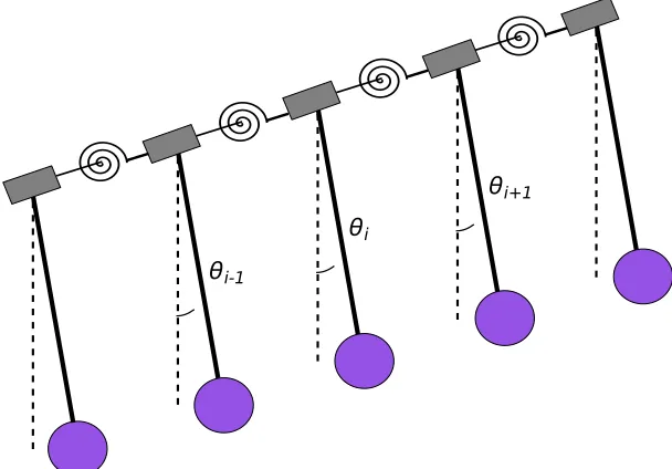
1.1 Pendulum hung from a support with its potential energy as a function of angular rotation. . . 1 1.2 Nonlinear lattice of rotating pendulums connected by torsional springs.

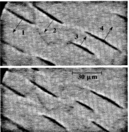
The pendulums rotate out of the plane creating the transition wave. . 2 1.3 Microstructure of the twinned martensite phase next to a

homoge-neous austenite phase in a Cu-Ni-Al alloy (adapted from [34]) . . . . 4 1.4 Axon in the peripheral nervous system covered with a myelin sheath

made up of Schwann cells. There are periodic gaps in the sheaths called the Nodes of Ranvier. The electrical signal passes through due to the potential difference between the Nodes of Ranvier (cour-tesy [115]) . . . 5 1.5 A Josephson junction . . . 6 1.6 A photoemission electron microscope image showing the oxidation of

CO on a Pt substrate. The dark regions is where the oxygen adsorbate is concentrated that move as localized waves with a constant velocity (adapted from [13]). . . 8 2.1 Bistable element consisting of two elastic springs and a point mass,

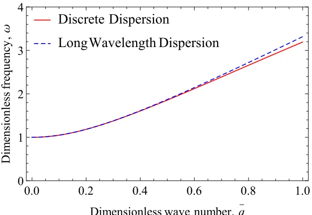
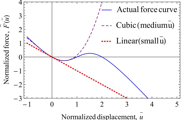
energyψ(u), and force F(u). . . 12 2.2 Periodic chain of bistable elements. . . 15 2.3 Dispersion relation comparison . . . 17 2.4 Nonlinear spring force and approximations introduced for the three

regimes for d =1. . . 18 2.5 Small-amplitude regime: numerical results compared to the linear

Klein-Gordon solution. . . 20 2.6 Small-amplitude regime: x-t-contour diagram of the numerical

so-lution; for comparison, the solid red line represents a positive char-acteristic of the theoretical solution. . . 21 2.7 Snapshots of the propagating wave (traveling from left to right) at

(12)

2.8 Discrete Fourier transform of the spatial variation of the waveform at a chosen instant of time. . . 27 2.9 Comparison of theoretical large-amplitude solution and

numerically-determined wave profile (for parameters d = 1, z0 = −93.2 and

v= 2.812). . . 28

2.10 x-t-contour diagram of the numerical solution for the large-amplitude regime. The red straight line is the best fit line till t = 250 corre-sponding to the leading edge characteristic. . . 29 2.11 The characteristic curve corresponding to the leading edge of the

wave is shown in comparison with the best-fit solution at t = 250. The slope of the line determines the initial speed of the propagating wave. This speed is used to compute the exact solution in the kink soliton propagation. The kink slows down toward the end due to the energy radiated by the oscillatory tail. . . 30 2.12 Energy landscape E(u) with positive and negative pre-deformation

as well as without pre-loads. . . 33 2.13 x-t-contour diagram of the numerical solution for a precompression

¯

u₀ = 0.03. The kink characteristic is relatively straighter than the characteristic without precompression. . . 33 2.14 (a) Wave profiles for ¯u0 = 0.3 and t3 > t2 > t1. (b) x-t-contour

diagram of the numerical solution for a precompression of ¯u0= 0.3. . 34

2.15 Variation of the kink propagation velocity with pre-compression for an initial (normalized) velocity of the first node of v0 = 4. The

dotted line shows the characteristic sound speed ¯c0of the medium for

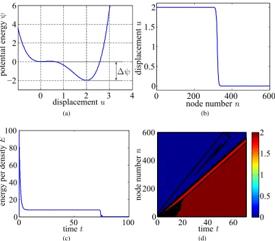
comparison. . . 35 3.1 Example of a moving transition wave: (a) bistable topology of the

(13)

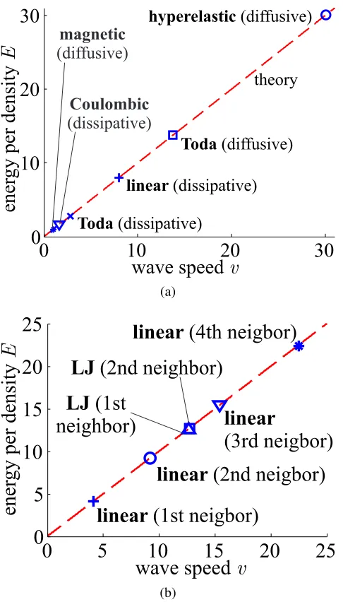
3.2 Plots of the kinetic energy E of the traveling wave vs. kink propa-gation speedv for (a) various examples of interaction potentials and (b) varying numbers of interacting neighbors. All examples use the bistable energy of Fig.3.1awithm= 1 for dissipative andm=0.0001 for weakly inertial or diffusive cases, anda= 1. All results lie almost perfectly on the predicted lines with slopes E/v = ∆ψ/2γ =1. . . 47 3.3 (a) Three different topologies of the on-site potentialψwith different

equilibrium distances but with the same energy jump∆ψ; (b) resulting energy per densityEvs. wave speedvfor the different topologies and interaction potentials (all other parameters as in Fig. 3.2). Again, all computed values fall onto the predicted line with slope E/v = ∆ψ/₂γ =_{1. . . .} ₄₈ 3.4 (a) The three possible topologies of a triple-well potential that

gen-erate propagating kinks: (I) ∆ψ1,∆ψ2 > 0, (II)∆ψ1 > 0, ∆ψ2 < 0,

and (III)∆ψ1 < 0 ,∆ψ1+∆ψ2> 0. (b) Resulting waveforms for the

three cases: (I) two transition waves travel with different velocities, (II) only one partial transition wave propagates (the other is stationary as∆ψ2 < 0), and (III) one complete transition wave propagates with

a constant velocity (the second transition drags the first along). . . . 49 3.5 (a) Displacement profile and (b) kinetic energy when discreteness

effects dominate and the wave profile is not smooth (m = 1000 with a hyperelastic interaction potential). . . 51 4.1 Tailored distribution of used bistable composite laminates. . . 56 4.2 (a) Force displacement curve of the bistable element for clamping

(14)

4.3 (a) The experimental lattice is shown along with the trigger magnet mounted on a precision screw. The displacements of elements 8 to 11 that are marked using a speckle pattern are tracked using a digital image correlation software (DIC). (b) A schematic of the experimental measurement technique is shown. The two cameras are synchronized and capture the 3D deformation field of the tracked specimens. The out-of-plane deformation is obtained using the Vic-3D DIC software. . . 59 4.4 Transition wave propagation for three different combinations of lattice

distance (L) and rail distance (R). The displacement time series is shown for the 8th - 11th element (blue diamonds, magenta squares, red 5 point stars and black 6 point starts respectively) for (a) L = 8 cm, R = 22.5 cm (b) L = 6 cm, R = 22 cm and (c) L = 8 cm, R = 21.5 cm. The negative values of the displacements indicate that the elements are deforming away from the camera. The direct numerical simulations of the discrete particle model Eq. (4.1) (dashed lines) are in good agreement with the experimental results (solid lines). The inset of each panel is the numerical solution of the exact transition wave. On reaching the boundary, the waves do not reflect back into the bulk and hence the transition is unidirectional. . . 60 4.5 Snap-shot sequence showing the transition wave as it propagates

through the experimental lattice. Images were acquired at 4000 fps. . 61 4.6 (a) Wave velocity as a function of lattice distance for different rail

distances. The dissipation parameter has been optimized such that the wave velocity matches for lattice distance 8 cm for rail distances 21.5 cm and 22 cm, and lattice distance 7 cm for rail distance 22.5 cm. (b) Full width at half maximum (FWHM) of the strain profile of the transition wave as a function of lattice distance for different rail distances. . . 62 4.7 (a) Variation of wave velocity with interaction coefficient p for

(15)

4.8 (a) Fitted onsite force for the case of R = 22.5 cm and L = 8 cm (dashed red line) and experimentally measured values (red markers). The symmetric counterpart of this function is also shown (blue solid line), which was obtained by modifying the local minimum and largest root along the linesr1andr2respectively. The fraction of the distance

moved along these lines is the asymmetry parameter . (b) Plot of the wave speed as the asymmetry parameter is varied. . . 66 4.9 Energy profile of a simulation for R=21.5 cm and L=8 cm. The

energy drops to zero when the wave reaches the end of the lattice. . . 69 5.1 (A) The system consists of a 1D series of bistable elements

con-nected by soft coupling elements (scale bar represents 5 mm); (B) the coupling elements are designed to exhibit a linear mechanical re-sponse, while (C-D), the bistable elements possess two stable states (scale bars represent 5 mm); the bistability originates from lateral constraint (d) on a beam pair that is displaced (x) perpendicularly to the constraint; the mechanical response is fully determined by the aspect ratio (L divided by the thickness of the beam) and d; the two stable configurations of the bistable element correspond to the displacements x = xs₁ = 0 and x = xs₀; (E) in certain cases a sta-ble nonlinear transition wave propagates through the system (with each bistable element undergoing a displacement from x = xs0 to

x = xs1); the instability ( ˆSi) propagates with constant velocity and geometry, enabled by both (i) the balance of nonlinear and dispersive effects and (ii) the balance of dissipation and energy release; here, we show snapshots of the evolving state of the chain, witht1= 0.128 s,

t₂ =0.194 s, andt3 =0.252 s relative to the start of the experiment,

in this case withd = 18.6 mm. . . 73 5.2 Using different geometries for the linear coupling elements leads to

(16)

5.3 (A) The shaker (left) was attached to an accelerometer that was directly glued to the samples; the accelerator used to measure the output was glued to the

other end of the sample; the acrylic braces (red) were used to hold the soft

architecture at well-defined widths, and were glued to the laboratory stands

to prevent unwanted movement; (B) small amplitude, linear excitation from

either end of the chain is rapidly dissipated due to the damping intrinsic

to the polymer, as is particularly evident with increasing frequency, shown

here for samples with 6, 15, and 50 bistable units. . . 77 5.4 The transition wave can be initiated anywhere along the chain, with

com-pressive and rarefaction pulses proceeding in opposite directions from the

point of initiation (hered =18.6 mm). (A-B) the normalized displacements of the individual bistable elements ( ˆxifor each of theielements in the chain) during the propagation of the wave, as recorded with a high speed camera at

500 Hz; these panels show the propagation of the transition with a constant

velocity and pulse width, after a brief initiation period during which

steady-state is established; (C-D) Optical images of the experiments during wave

propagation (obtained from a high-speed camera), corresponding to the data

in panels A-B; (E-F) Simulations corresponding to the experiments shown

in panels A-B, showing excellent quantitative agreement; for the

compres-sion initiated pulse, the initiating displacement of the wave takes place on

the left of the chain and is in the same direction as the pulse propagation;

for the tension initiated pulse, the initiating displacement takes place on

the right of the chain, and the local tensile displacement is in the opposite

direction of the wave propagation. . . 79 5.5 (A) An example of the beam deformation simulation is shown. All

sim-ulations were performed on only one half of the bistable element (i.e., on

one tilted beam). Different configurations of the beam are shown as it

is displaced from one stable configuration to another. The force at node

’B’ is measured (and doubled to account for bistable element consisting

of two tilted beams). (B) The numerical, experimental and best-fit

force-displacement curves are shown for d = 17.5 mm. The graphics indicate that experimental and numerical results are in good agreement. . . 81 5.6 (A-B) Experimental and simulation results, respectively, corresponding to

(17)

5.7 (A) The on-site potential as a function of xandd, as determined via quasi-static 1D displacement-controlled simulations of an individual bistable

el-ement; (B-C) Simulated values of pulse velocity and pulse width,

respec-tively, as a function of end-to-end distancedand connector stiffnessk; (D) The measured energy landscape (panel A) of the individual bistable

ele-ments is combined with the simulated pulse widths (panel C) to compute an

approximate energy barrierEt ot for the entire propagating pulse (a function of bothdandk). . . 83 5.8 Experimental data obtained by directly measuring the force-displacement

behavior of a single bistable element for different lateral constraints,d; the potential energy is calculated from this, showing a large effect of don the energy barrier of the bistable elements. . . 85 5.9 (A) Experiments show that when d is small (17.5 mm here) the energy

barrier between the two stable states is larger and the wave propagation is

slower; (B) when d is larger (18.6 mm here) the smaller energy barrier allows a larger propagation speed, as evidenced by the changed slope. . . . 85 5.10 Because the system is deformable, different values ofd can be used along

the length of the system, resulting in spatially-varying energy barriers to

propagation; this can be used to vary the velocity along the length of the

chain, as it is here for a gradient structure (d is about d1 = 14.5 mm at

the left end and about d2 = 19.0 mm at the right end, corresponding to

measured speeds of 0.8 and 5.2 m/s, respectively). . . 86 5.11 (A) Whenk is high (2100 N/m here) experiments show that both the pulse

width and the pulse velocity (as determined by the slope) are much higher,

even with the same value ofd(18.6 mm), than (B) whenk is low (80 N/m here); (C) this same comparison can be made by taking experimental

snap-shots of the two different systems (k=80 N/m andk=2100 N/m, correspond-ing to the differences in morphology of these elements, as pictured in the

(18)

5.12 (A) A functional soft mechanical diode can be realized by creating a het-erogeneous chain comprised of a region with soft connectors and a small

energy barrier (left) and a region with stiff connectors and a large energy

barrier (right); a pulse initiated in the soft region (from the left) cannot pass

into the stiff region due to the large energy barrier, causing the pulse to

freeze indefinitely at the interface (panel A, windowsiv−viand panel A); in contrast (panel A, windowsvii-ixand panel (C) when the pulse is initiated

in the stiff region the propagation continues into the soft region and through

the whole chain without interruption. . . 89 5.13 (A) A bifurcated chain demonstrating tunable logic in a soft mechanical

system; the distancedoutdetermines the logical behavior, producing either

an AND or an OR gate from the same system; (B) when dout is small

(in this case 16.7 mm) the energy barrier is higher, and both input chains

must be transitioned in order for the wave to propagate through the output,

comprising the function of a logical AND gate; (C) by increasing dout

(to 18.6 mm in this case), the energy barrier to continue propagation in

the output chain decreases in a predictable manner, producing logical OR

behavior in which a transition wave in either input chain has sufficient energy

to initiate propagation in the output chain. . . 91 6.1 Phase diagram of PZT. (The figure has been adapted from [23]) . . . 98 6.2 (a) Cubic structure of PZT below the Curie temperature. (b)

Tetrago-nal structure of PZT above the Curie temperature. (adapted from [161]) 98 6.3 Four of the six Variants of PZT. The other two variants have

polar-izations into the plane and out of the plane (adapted from [161]). . . . 99 6.4 Schematic view of a 180◦domain wall in a single-crystal ferroelectric

ceramic capacitor with applied electric fieldeparallel to the domain wall that is moving with a velocityv. . . 100 6.5 (a) Plot of equilibrium polarizations p+ and p− as functions of the

applied electric field. The inset shows the energy W for a given electric fieldey with p− and p+ as its local minimizers. p± coincide for e ≥ ec. (b) Comparison between the simulated profile of the polarization for a stationary domain wall and the hyperbolic tangent approximation. As can be seen, the arc-tangent profile accurately represents the variation of polarization across the domain wall. . . 103 6.6 A comparison between theory and numerical simulations of the

(19)

LIST OF TABLES

Number Page

3.1 Numerical results for the sixth-order tri-stable potential energy with energy differences ∆ψ1 (first) and∆ψ2 (second well). Wave speeds

vi (identified from contour plots by a linear regression fit) and total

kinetic energies E are compared to the superposed theoretical pre-dictions of the linear energy law (recall that travelling waves require ∆ψi > 0). . . 50 4.1 Geometric properties of the sections composing the spatially varying

fiber for the bistable elements. Refer to for the schematic representa-tion in Fig.4.1of the given parameters. . . 56 4.2 Material properties for a typical ply of CFRP c-m-p (CM-Preg

(20)

C h a p t e r 1

INTRODUCTION

The goal of this thesis is to understand the physics of nonlinear wave propagation in systems that exhibit multiple states or ‘phases’ of equilibrium. The switching between two stable equilibria gives rise to a nonlinear wave called a transition wave and the phenomenon is called a phase transition. This thesis explores the theory behind these phase transitions in conservative, dissipative and diffusive systems. Further, we investigate how the theory can be used to design and experimentally realize nonlinear mechanical systems having structural phase transitions. We also discuss the application of the theory to current models of microstructure evolution in ferroelectric ceramics and suggest further steps to improve the model. This chapter introduces the concept of phase transitions and their mechanism in various systems.

1.1 Motivation

A phase transition can be illustrated by a simple example in mechanics. Consider a pendulum with a mass, hanging from a rigid support. Assuming the bar of the pendulum is mass-less, the potential energy of the hanging mass as a function of the angle of rotation is shown in Fig.1.1. The energy has a multi-stable landscape having an equilibrium for every 2π rotation. An infinite lattice of such pendulums can be built by connecting them through a linear torsional springs. A schematic of

θ

potential energy

ψ

(θ)

(21)

this lattice is shown in Fig.1.2. The governing equation for the motion of the nt h pendulum is given by

Iθ¨_n−C(θn+1−2θn+θn−₁)+mglsinθn =0, (1.1)

where I is the moment of inertia, C is the stiffness of the torsional springs, m is the mass, gis the acceleration due to gravity and l is the length of the pendulum. The rotation of one of the pendulums from one stable state to another (i.e. θ = 0 → 2π) causes a traveling wave to propagate through the system that switches each consecutive pendulum from θ = 0 phase to theθ = 2π phase in a sequential manner. This mechanical system was designed by Scott [130], as a simple model of the nonlinear Klein-Gordon equation, where he analyzed the nature and stability of the transition wave. Further numerical and experimental investigations were performed to characterize transitions in this system [32, 38, 102]. The presence of the multi-stable potential creates topological wavefronts or kinks that can travel through the medium. Phase transformations due to the propagation of such a kink or transition front are ubiquitous, occurring in varied systems. Following are a few examples where phase transitions are commonly encountered due to the presence of bi/multi-stable potentials in lattices or continua.

(22)

1.2 Lattice dynamics in mechanics

Equation (1.1) is the celebrated Frenkel-Kontorova (FK) equation that was first em-ployed to explain dislocation motion in metals [51]. The dynamics of the kink in the model describes the propagation of the dislocation core. In contrary to a contin-uum, the inherent discreteness of the lattice gives rise to the Peierls-Nabarro (PN) potential that the kink needs to overcome in order to move in the lattice [96, 112]. Such effects of discreteness of the lattice along with acoustic radiation [7], prefer-ential velocity of propagation [114], and kink dressing or shape modification [59] have been studied in great detail. For a review of FK lattice models, see [26, 27]. FK-type lattice models have been used to explain other mechanical processes as well. For instance, in structural mechanics, chains of bistable linkages with gaps of zero resistance or a "waiting link structure" have been shown to have increased stability due to the delocalization of damage and conversion of mechanical energy to heat through high-frequency background oscillations [31, 139]. Such periodic chains with bistable linkages or non-monotonic stress-strain relationships have been successfully employed as models to explain structural transitions, fracture, and dam-age [9, 10,69, 138,150, 154]. The mechanical response of carbon nanotubes [20, 48] have also been explained on the basis of buckling or snapping instabilities aris-ing from systems with multiple stable configurations described by lattice models. Stochastics coupled with multi-stable on-site potentials in the Langevin framework have been used to develop models for surface friction [158, 159]. Therefore, FK lattice models have been utilized to explain mechanical processes from the small scale like surface friction to large-scale structural mechanics.

1.3 Thermoelastic materials

(23)

Figure 1.3: Microstructure of the twinned martensite phase next to a homogeneous austenite phase in a Cu-Ni-Al alloy (adapted from [34])

thermoelastic solid undergoing a phase transition in a one-dimensional setting has been extensively studied [2, 3, 5]. A key result from these papers is the entropy inequality for phase transformations,

f(t)s(t)˙ ≥ 0, (1.2)

(24)

Figure 1.4: Axon in the peripheral nervous system covered with a myelin sheath made up of Schwann cells. There are periodic gaps in the sheaths called the Nodes of Ranvier. The electrical signal passes through due to the potential difference between the Nodes of Ranvier (courtesy [115])

.

for many applications such as vibration damping in aircrafts [54], control of civil structures [141] and dental braces in medicine [86].

1.4 Action potential propagation through myelinated axons

Transition waves in the form of propagation of electrical signals also occur in biological systems. One such example is the propagation of action potentials along the axon of a nerve cell. An axon is a transmission line that communicates between two neurons. A diagram of an axon in the peripheral nervous system is shown in Fig. 1.4. For efficient communication, the axon is covered by myelin sheaths composed of glial cells called Schwann cells in the peripheral nervous system and oligodendrocytes in the central nervous system [115]. The presence of the myelin sheaths increases the effective resistance of the membrane from 103Ωcm2to 105Ω cm2 and reduces the capacitance from 10−6 µF/cm2 to 10−8 µF/cm2, causing fast signal propagation [65]. The sheaths are separated by periodic gaps called Nodes of Ranvier. The electrical signal jumps from one node to another in the form of a transition wave that is given by the equation,

dVn

dt = D(Vn+1−2Vn+Vn)+ f(Vn), (1.3)

(25)

nerve fibers was performed by Hodgkin and Huxley on the nerve [55]. Another model to simulate the motion of the transition wave was proposed by Fitzhugh, which was later realized experimentally through an electrical circuit by Nagumo et. al. [45, 100]. For a general discussion of electrophysics of nerve fibers, see [65, 115,131].

1.5 Josephson junctions

The Josephson junction that shows current tunneling through an electric insulator was proposed by Brian Josephson as part of his PhD work for which he was awarded the Nobel Prize in Physics in 1973 [62]. A schematic of a Josephson junction is shown in Fig.1.5.

Superconductor

Insulator

Figure 1.5: A Josephson junction

The Josephson junction consists of an insulator sandwiched by two superconducting electrodes. The superconductor has pairs of bound electrons with two spins of±1/2 called Cooper pairs which have an electromagnetic quantum phase associated with them. For a short Josephson junction, if the phase difference between the Cooper pair phases of the two superconductors isφ, then the equation governing the phase difference is of that of a damped oscillatory pendulum, written as

d2φ

dt2 +

1 RC

dφ dt +ω

2

0sinφ= JB, (1.4)

where R is the resistance, C is the capacitance, ω0 is a characteristic frequency

(26)

(27)

Figure 1.6: A photoemission electron microscope image showing the oxidation of CO on a Pt substrate. The dark regions is where the oxygen adsorbate is concentrated that move as localized waves with a constant velocity (adapted from [13]).

reactors arranged in a ring [22]. The system shows propagation failure below a certain critical coupling constant very similar to the propagation failure in a nerve fiber [73].

Therefore, phase transitions due to the propagation of strongly nonlinear transition waves occur in many physical, chemical, and biological bistable systems as a result of inter-well switching. This thesis explores this phenomenon to characterize this wave propagation that occurs in these different systems.

1.7 Outline

(28)

pre-compression applied to each node of the lattice, we show that the wave propagation is a combination of the strongly nonlinear kink shaped wave mode and the weakly nonlinear envelope solitary wave mode. This chapter provides a direction towards the creation of nonlinear metamaterials.

Chapter3analyzes inter-well phase transitions in a lattice and continuum when the mechanism is diffusive or dissipative in nature in general bi/multi-stable lattices and continua. Unlike the conservative case where there is a family of kink solutions, we observe that there is at most one steady-state waveform and velocity. The average energy of the wave is linearly related to its velocity through a universal principle. The ratio of the average energy to velocity is independent of the bistable topology, number of neighborhood interactions, and form of the interaction potential. We also show that this energy scaling applies to a multi-stable switching as well. We confirm our theory with multiple numerical examples.

Chapter4 delineates a design of a fully nonlinear discrete dissipative system with on-site bistable nonlinearities and interaction nonlinearities. The system allows the propagation of strongly nonlinear transition waves. We show that, in such a system, in spite of discreteness effects and highly nonlinear interactions, the average energy per momentum density transported by the transition wave remains a constant and can be determined by the energy law derived in the previous chapter. Due to the asymmetry in the energy wells, the wave propagation is unidirectional in nature, so that the transition occurs only from the high-energy state to the low-energy state.

Chapter5describes a structural application of the theory to build soft mechanical metamaterials that counteract dissipation with structural instabilities. We present a lattice made of a polymeric material that propagates transition waves while linear waves are damped out by the intrinsic dissipation. The structural properties can be readily tuned by applying pre-compression to the lattice to propagate the waves faster or slower. The properties of the lattice can be spatially altered to give rise to accelerating and decelerating waves. A design to realize soft mechanical logic such as diodes, AND, and OR gates is also described. This chapter presents a blueprint for novel metamaterial applications in the nonlinear regime of wave propagation.

(29)

(30)

C h a p t e r 2

NONLINEAR DYNAMICS OF A CONSERVATIVE LATTICE

WITH ON-SITE BISTABLE POTENTIALS

Research presented in this chapter has been adapted from the following publication:

Neel Nadkarni, Chiara Daraio, and Dennis M. Kochmann. “Dynamics of periodic mechanical structures containing bistable elastic elements: From elastic to solitary wave propagation”. In: Physical Review E 90.2 (Aug. 2014), p. 023204. doi: 10 . 1103 / PhysRevE . 90 . 023204_{. url:} http : / / link . aps . org / doi / 10 . 1103/PhysRevE.90.023204_.

In this chapter, we analyze the problem of phase transitions and intra-well dynamics in a conservative system that permits two stable states at each node through a bistable on-site potential. In particular, we investigate the nonlinear dynamics of a periodic chain of bistable elements consisting of masses connected by elastic springs whose constrained arrangement gives rise to a large-deformation snap-through instability. We show that the resulting negative-stiffness effect produces three different regimes of (linear and nonlinear) wave propagation in the periodic medium, depending on the wave amplitude. At small amplitudes, linear elastic waves experience dispersion that is controllable by the geometry and by the level of precompression. At moderate to large amplitudes, solitary waves arise in the weakly and strongly nonlinear regime. For each case, we present closed-form analytical solutions and we confirm our theoretical findings by specific numerical examples. The precompression reveals a class of wave propagation for a partially positive and negative potential. The presented results highlight opportunities in the design of mechanical metamaterials based on negative-stiffness elements, which go beyond current concepts primarily based on linear elastic wave propagation. Our findings shed light on the rich effective dynamics achievable by nonlinear small-scale instabilities in solids and structures.

2.1 Introduction

(31)

L

d/2

u

y

(

u

)

u

-

F

=

y¢

(

u

)

L

k

1

k

1

m

Figure 2.1: Bistable element consisting of two elastic springs and a point mass, energyψ(u), and force F(u).

162], acoustic lenses and diodes [17,142], sound isolators and sensors [118, 172], and acoustic cloaks and sonar stealth technologies [92,94]. Design strategies com-monly exploit the scattering of elastic waves in periodic media at characteristic frequencies in all or specific directions [72,125, 137] as well as resonant phenom-ena capable of absorbing energy on lower scales by local resonators [83, 134]. In all these examples, the careful microscale periodic architecture of multiscale en-gineered material systems leads to an interesting or beneficial effective dynamic behavior on the macroscale. Besides pronounced acoustic band gaps [128, 167], this design paradigm has resulted in negative effective dynamic stiffness [42] and mass density [84, 166], and combinations of both [37]. Here, negative stiffness and negative mass density refer to the effective dynamic properties: An elastic sys-tem containing only positive-stiffness elements can demonstrate negative effective dynamic quantities near resonance.

(32)

solids and structures also promise interesting nonlinear dynamic effects, including solitary-wave propagation, which provides opportunities to focus acoustic signals in mechanical metamaterials [50,142]. Homogeneous solids undergoing finite elastic deformation [111] as well as periodic media experiencing nonlinear elastic insta-bilities [16] have been shown to exhibit acoustic band gaps that are controllable by the amount of nonlinear pre-deformation, yet the investigated waves again op-erate in the linear elastic regime. To date, only one example of periodic elastic mechanical system (as illustrated in Sec.1.1) has been reported that produces sine-Gordon solitons by allowing a kink propagation in the form of elastically connected rotating pendulums [32, 38, 102, 127, 130]. The weakly or strongly nonlinear re-sponse of elastic media containing negative-stiffness elements such as the bistable spring configuration shown in Fig. 2.1 has remained widely unexplored, in part because such instabilities in solids and the resulting nonlinear effective dynamics are mathematically complex and make analytical solutions a rare find.

Here we study a mechanical system capable of propagating impact pressure waves in three different regimes, serving as a model for the creation ofnonlinear acoustic metamaterialswith static negative-stiffness elements. We present closed-form

(33)

(34)

(35)

(36)

(37)

(38)

corresponds to an unstable equilibrium configuration of the system. The smallest perturbation is sufficient to cause the system to snap into either energy well and thus to transform the scenario into either the ¯u >1 or the ¯u< 1 case.

In the following sections, we will investigate the wave propagation behavior in all three regimes. To confirm our theoretical solutions, we will compare to numerical results obtained for the example parameters d = 1, T = 1 and Kr = 10, from which the three regimes are chosen as (i) |u| ≤¯ 0.05, (ii) |u| ≤¯ 0.3, and (iii) |u| ≤_¯ 2. Convincing agreement has been verified for various combinations of these

parameters, for brevity we here present only this specific case.

Numerical solutions are obtained from a chain of 100 elementary unit cells modeled in the time domain by an implicit finite difference scheme of Newmark-β type with parameters chosen to minimize numerical damping (β = 0.25, γ = 0.5). Displacement and/or velocity boundary conditions are directly imposed on the first node of the chain, while the remaining nodes may vibrate freely. All nodes are constrained to only move horizontally.

2.6 Small amplitude: linear solution 2.6.1 Analytical solution

The equation governing the wave propagation in this regime is given by

¯

u,¯tt¯−c¯₀2u¯x¯x¯+ω2₀u¯ =0, (2.23)

withω2₀from (2.16). This is the dimensionless Linear Klein-Gordon equation [35] for the unknown displacement field ¯u(x¯,t)¯ . The theoretical solution for this problem is of the form

¯

u(x¯,t¯)= A cos(q¯x¯−ω¯t¯)+B sin(q¯x¯−ω¯t¯), (2.24)

where the dimensionless wave number ¯qand the dimensionless angular frequency ¯ω are related by the dispersion relation (2.19). Therefore, this regime admits the prop-agation of linear elastic waves at frequencies outside the stop bands characterized by the dispersion relations.

2.6.2 Numerical results

For the numerical benchmark test, the first node of the chain of bistable elements is excited by time-harmonic displacements (we enforce displacement and correspond-ing velocity boundary conditions at the first node) accordcorrespond-ing to

¯

(39)

(40)

an equation of Cubic Nonlinear Klein-Gordon-type [67, 116] for the unknown displacement field ¯u(x¯,t)¯ . The solution can be found by a perturbation multiple-scales expansion [103]. Therefore, we use the ansatz

¯

u(x¯,t)¯ = φ₀(x¯,t¯)+2φ

1(x¯,t)¯ +3φ2(x¯,t)¯ +O(4), (2.27)

where || 1 is a small characteristic length scale. For the current problem, the expansion is restricted to third order, since this approximation demonstrates sufficient accuracy for the medium amplitude regime, cf. Section2.5. Suppose that in addition to variables ¯xand ¯t, the solution depends on multiple scales of position and time. Then, new scaled variables can be defined by

Xi =ix¯ and Ti= it¯. (2.28)

Again, we limit scales to order three. Consequently, we now seek solutions

φi(x¯,t)¯ = φi(X₀,X₁,X₂,T₀,T₁,T₂). (2.29)

Derivatives with respect to the primary variables become

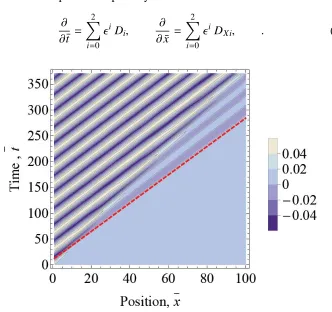
∂ ∂t¯ =

2

X

i=₀

i

Di,

∂ ∂x¯ =

2

X

i=₀

i

DXi, . (2.30)

(41)

(42)

(43)

(44)

(45)

0 50 100 150 200

-0.4

-0.2 0.0 0.2 0.4

Position, x

Displacement

,

u

H

x

L

T=t1

T=t2

T=t3

T=t4

Figure 2.7: Snapshots of the propagating wave (traveling from left to right) at different instances of time show the evolution of the envelope soliton. The sech-type envelope begins to form due to self-modulation, as the wave passes through the lattice.

a discrete Fourier transform, Hann, Blackman and Hamming windows are used to determine the spectral content of the signal. The resulting peak frequency corresponds to the spatial wave number of the applied frequency. However, side lobes form which can be explained by the modulational instability [168] caused by the weakly-nonlinear effects discussed above. Hence, wave propagation in this regime can indeed be explained by the Non-Linear Schrödinger and the Cubic Non-Linear Klein-Gordon equations, and numerical results confirm the theoretical prediction of an envelope soliton. The envelope appears to vary as it moves along the chain; yet, the waveform preserves it localized nature, leaving behind small-amplitude high-frequency oscillations.

2.8 Large amplitude: strong nonlinearity 2.8.1 Analytical solution

For the case of large amplitudes, we use the exact nonlinear form of the potential energy. Therefore, the governing equation in the continuum limit is

¯

ut_¯t¯−c¯₀2u¯x¯x¯−F¯(u)¯ = 0. (2.58)

For convenience, the over-bars are omitted in the following. We seek a traveling wave solution of the form u(x,t) = u(x −vt) = u(z), where v is the propagation velocity andz= x−vta reduced variable. Substitution into (2.58) gives

(v2₋_c2

(46)

(47)

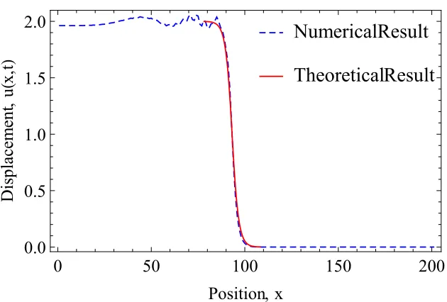
NumericalResult

TheoreticalResult

0 50 100 150 200

0.0 0.5 1.0 1.5 2.0

Position, x

Displacement

,

u

H

x,

t

L

Figure 2.9: Comparison of theoretical large-amplitude solution and numerically-determined wave profile (for parametersd =1, z0= −93.2 andv =2.812).

In summary, the solution in the large-amplitude case is indeed a propagating wave of typeu(x,t) = u(x −vt). From (2.64) we conclude that c0 > v which implies

that the wave speed is subsonic. Although (2.64) cannot be inverted to solve for u(z) explicitly, the relation shows that u(z) → 0 as z → ∞ and that u(z) → 2

as z → −∞. In addition, the function can be plotted parametrically foru ∈ (0,2), which is shown in Fig.2.9. Obviously, the wave front is localized and of kink soliton type, which can be physically explained by the snap-through effect of each spring from one stable configuration to the other. The shape of the kink depends on the velocity of propagation with higher velocity kinks having steeper slopes.

2.8.2 Numerical results

(48)

Figure 2.10: x-t-contour diagram of the numerical solution for the large-amplitude regime. The red straight line is the best fit line tillt = 250 corresponding to the leading edge characteristic.

that the velocity is not constant but variations with time are marginal so that we may assume the wave is traveling at almost constant speed. Inserting the propagation velocity into the theoretical solution shows an excellent match with the numerical wave profile, which confirms the accuracy of the aforementioned analytical solution for the large-amplitude regime. The propagating wave is of anti-soliton nature with a topological charge of−1.

2.8.3 Energy of the kink soliton

Bistable elements have been shown to produce twinkling which results in energy dissipation, see e.g. ref. [44] and references therein. Here, we disregard just oscil-lations and focus on the propagating kink soliton whose energy can be determined by integrating the Hamiltonian spatial density over the complete lattice at any given time. The Hamiltonian density per unit spacing in the continuum limit is given by

h(x,t)= 1 2u

2

t + 1₂c2₀u2x+ψ(u). (2.66)

In the large-amplitude case as derived in Sec.2.8.1, we haveu(x,t) = u(x−vt) = u(z). Substitution into (2.66) gives

h(z) =*

,

v2+_c2 0

2 +

-u2

(49)

(50)

(51)

(52)

u

0

=

0.3

u

0

=-

0.2

u

0

=

0

-2 -1 0 1 2 3 4

-0.5 0.0 0.5 1.0 1.5 2.0 2.5 3.0

Displacement, u

Modified

energy

,

E

H

u

L

Figure 2.12: Energy landscapeE(u)with positive and negative pre-deformation as well as without pre-loads.

in Fig.2.13 confirms that the kink characteristic is now linear and hence the kink has stabilized as compared to the case without precompression, cf. Fig.2.10.

Increasing the pre-compression creates a combination of a kink and trailing oscil-lations which are localized as the wave moves through the chain. After attaining a

Figure 2.13: x-t-contour diagram of the numerical solution for a precompression ¯

(53)

0 50 100 150 200 0.0

0.5 1.0 1.5 2.0 2.5

Position of nodes, x

Displacements

,

u

H

x

,t

L

t1

t2

t3

(a)

(b)

Figure 2.14: (a) Wave profiles for ¯u0 =0.3 andt3 >t2 >t1. (b)x-t-contour diagram

of the numerical solution for a precompression of ¯u0= 0.3.

(54)

0.0 0.1 0.2 0.3 0.4 2.6

2.7 2.8 2.9 3.0 3.1 3.2

Precompression, u0

Wave

propagation

velocity

,

v

Figure 2.15: Variation of the kink propagation velocity with pre-compression for an initial (normalized) velocity of the first node of v0 = 4. The dotted line shows the

characteristic sound speed ¯c0of the medium for comparison.

the direction of snapping results in the snapped potential well having lower energy. Consequently, after snapping every mass has residual kinetic energy. This energy, however, is insufficient for a spring to snap back since part of the energy is carried away by the kink soliton. Hence, the masses oscillate in the snapped well with a medium amplitude giving rise to localization by modulational instability as seen in the envelope soliton case in Section2.7. For these reasons, the pre-deformation results in a combination of the two modes of kink and envelope soliton propagation with an envelope soliton-like wave created behind the kink. As may be expected, the velocity of the propagating wave front increases with increasing pre-compression for a constant input of energy as shown in Fig.2.15. There is a sharp rise in the velocity of propagation for small pre-compressions followed by a fairly linear increase for large pre-compressions, ultimately becoming supersonic.

2.10 Conclusions

(55)

all three regimes, we have derived analytical solutions of the displacement field in the continuum limit and we have demonstrated excellent agreement with the numerical solution obtained from a discrete chain of bistable elements. Wave propagation characteristics can be controlled by fine-tuning the geometric details of the bistable elements. Moreover, precompression brings the bistable elements closer to their snapping instability and hence can be used to control the wave propagation. We discussed the influence of precompression in all three amplitude regimes.

(56)

C h a p t e r 3

NONLINEAR DYNAMICS OF DISSIPATIVE AND DIFFUSIVE

PHASE TRANSITIONS

Neel Nadkarni, Chiara Daraio, Rohan Abeyaratne, and Dennis M. Kochmann. “Uni-versal energy transport law for dissipative and diffusive phase transitions”. In: Physi-cal Review B93.10 (Mar. 2016), p. 104109. doi: 10.1103/PhysRevB.93.104109.

url: http://link.aps.org/doi/10.1103/PhysRevB.93.104109.

In the previous chapter, the lattice of bistable elements was conservative in nature. In this chapter, we analyze the nonlinear mechanics of phase transitions in lattices that are governed by dissipative or diffusive dynamics. We present a scaling law for the kinetic energy and speed of transition waves in such media. By considering uniform discrete lattices and continuous solids, we show that, for arbitrary highly-nonlinear many-body interactions and multi-stable on-site potentials, the kinetic energy per density transported by a planar transition wave front always exhibits linear scaling with wave speed and the ratio of energy difference to interface mobility between the two phases. We confirm that the resulting linear superposition applies to highly-nonlinear examples from particle to continuum mechanics.

3.1 Introduction

(57)

(58)

(59)

(60)

(61)

(62)

(63)

(64)

(65)

(iii) Dipole-dipole interactions in a chain of magnets: V0(u)= F0(u/a+1) −₄

with (F0=0.016 anda= 5),

(iv) Nonlinear Toda interactions describing, among others, charge density waves [56]: V0(u) = F₀(1−e−βu/a)(withF0= 100,a =6 and β =6),

(v) Hyperelastic rubber connectors (1D incompressible Neo-Hookean solid [107]): V0(u) = F₀1+ _au −(u/a+1)−2

(withF0 =1 anda =6), and

(vi) Lennard-Jones (LJ) atomic interactions with varying cut-off radius: V0(u) = F₀f(1+u/a)−7−(1+u/a)−13

g

(withF0=137.17 anda =3).

Due to the short-range nature of LJ, we also computed results for long-range linear-spring interactions with up toNb=4 neighbors. The summary of results in Fig.3.2 confirms that the scaling law is indeed independent of the interaction potential and of the number of neighboring interactions.

Surprisingly, the scaling law is independent of the topology of the non-convex potentialψ. For verification, simulations were carried out on lattices with the three bistable interaction potentials shown in Fig. 3.3; all are fourth-order polynomials with the same value of∆ψ = 2. In analogy to Fig. 3.2, Fig.3.3b shows the linear relation between the computed kinetic energy of the traveling wave and the wave speed for all three bistable potentials, which confirms the energy transport law.

Since the energy law is linear, superposition can be expected in case of multi-well transitions despite the highly-nonlinear scenario. This suggests that a multi-well transition can be broken down into individual bi-stable transitions and analyzed separately to determine the total energy transported. To test this hypothesis, numer-ical experiments were performed for transitions occurring in a triple-well energy landscape as shown in Fig. 3.4. Results for three different interaction potentials are summarized in Table3.1 and show excellent agreement with deviations of less than 1%, thus confirming that superposition applies indeed. However, as seen from Fig. 3.4b, in the special case ∆ψ1 < 0 and∆ψ1+∆ψ2 > 0, the second transition

(66)

(67)

0

2

4

6

−2

0

2

4

6

displacement

u

y

_A

potential ener

gy

y

_B

y

_C

Dy

(a)

0

5

10

0

2

4

6

8

10

wave speed

v

ener

gy per density

E

hyperelastic + y

A

hyperelastic + y

_B

hyperelastic + y

_C

linear + y

A

linear + y

_B

linear + y

C

y

_B

y

C

magnetic

dipoles +

y

_A

theory

(b)

(68)

(69)

Interaction ∆ψ1 ∆ψ2 v1 v2

∆ψ₁v₁+∆ψ₂v₂

2γ E

Linear

0 2 4.5051 4.5051 4.5051 4.5029

0.5 1.5 5.6130 5.6130 5.6130 5.6146

1 1 7.2538 5.6741 6.4640 6.4114

1.5 0.5 8.1123 3.1141 6.8628 6.8637

2 0 8.5710 0.0307 8.5710 8.5760

Hyperelastic

0 2 1.4241 1.4240 1.4241 1.4231

0.5 1.5 1.7733 1.7732 1.7732 1.7697

1 1 2.2778 1.7762 2.0270 2.0089

1.5 0.5 2.5308 0.9760 2.2421 2.1424

2 0 2.6660 0.0132 2.6660 2.6670

Coulombic

0 2 0.9434 0.9434 0.9434 0.9429

0.5 1.5 1.1476 1.1476 1.1476 1.1480

1 1 1.4635 1.1492 1.3064 1.2964

1.5 0.5 1.6398 0.6307 1.3875 1.3877

2 0 1.7454 0.0000 1.7454 1.7464

(70)

0

200

400

600

0

1

2

node number n

displacement

u

(a)

0

50

100

0

1

2

3

time

t

ener

gy per density

E

4

×

10

(b)

Figure 3.5: (a) Displacement profile and (b) kinetic energy when discreteness effects dominate and the wave profile is not smooth (m = 1000 with a hyperelastic interaction potential).

whereF(un,t) is a generalized drag force. Following a similar procedure as that of Sec.3.2.1shows that

v∆ψ = −1 a

Z ∞

−∞

F(−vu,ξ)vu,ξdξ '

N

X

n=₁

F(un,t)un,t. (3.26)

(71)

law forces the dissipation to constantly drain energy from the system,

N

X

n=1

F(un,t)un,t ≥ 0 ⇒ v∆ψ ≥ 0. (3.27)

The above result is analogous to the entropy condition in phase boundary propa-gation [3], where∆ψ is the driving force on the phase front. Therefore, the above analysis may be interpreted as a derivation of the entropy condition for phase bound-ary propagation, in a general case. In the common case of linear damping, the power dissipated is proportional to the kinetic energy transported by the phase boundary. It is interesting to note that for linear on-site damping the dissipation removes only the contribution of the potential energy while preserving the kinetic energy.

3.5.2 Higher dimensions

Even though formulated in 1D, the above concepts also apply to general plane waves in higher dimensions. Consider, e.g., the time evolution the polarization vector p, a diffusive phase-field variable, in ferroelectric ceramics. The potential energy density is commonly written asW =ψ(p)+ κ₂|∇p|2with non-convexψ(p)and the nonlocal term representing energy stored in ferroelectric domain walls. One often derives the kinetics of domain switching from the gradient flow assumption [144, 170] with a drag coefficientγ, i.e.

γ ˙p=−δ_δW p = −

∂ψ ∂p +κ∇

2_p.

(3.28)

Ferroelectric switching is accommodated by the motion of planar domain walls which can be expressed as a plane wave p(x,t) = p(x · k − vt) = p(ξ), so that (3.28) becomes

− κ|k|2_p

i,ξξ −vγpi,ξ+ψ,i =0, (3.29)

using indicial notation. Thus we recover the general form of governing equa-tion (3.2). Multiplying by pi,ξ and integrating over time with pi,ξ = 0 as ξ → ±∞ yields

vγ Z ∞

−∞

pi,ξpi,ξdξ =∆ψ, (3.30)

(72)

field e, and mechanical strain ε all represented as moving transition waves). A detailed derivation is shown in Chapter 6 as to how this theory can be used to calculate the velocity of domain walls. In summary, even though derived for 1D systems, the applicability of the energy scaling law is more general and applies to plane waves in both discrete and continuous systems.

3.6 Conclusions

(73)

C h a p t e r 4

UNIDIRECTIONAL TRANSITION WAVES IN DISCRETE

BISTABLE LATTICES WITH NONLINEAR COUPLING

Neel Nadkarni, Andres F. Arrieta, Christopher Chong, Dennis M. Kochmann, and Chiara Daraio. “Unidirectional Transition Waves in Bistable Lattices”. In: Physical Review Letters116.24 (June 2016), p. 244501. doi: 10.1103/PhysRevLett.116. 244501_{. url:} http://link.aps.org/doi/10.1103/PhysRevLett.116. 244501_.

We present a model system for strongly nonlinear transition waves generated in a periodic lattice of bistable members connected by magnetic links to study the kind of discrete dissipative phase transitions discussed in Chapter3. The asymmetry of the on-site energy wells created by the bistable members produces a mechanical diode that supports only unidirectional transition wave propagation with constant wave velocity. We theoretically justify the cause of the unidirectionality of the transition wave and confirm these predictions by experiments and simulations. We further identify how the wave velocity and profile are uniquely linked to the double-well energy landscape, using the energy transport law as derived in Chapter3.

4.1 Introduction

(74)

impact shock waves have remained largely unexplored, partly due to their mathe-matical complexity and limited experimental realizations. Only one macroscopic experiment that has verified stable nonlinear transition waves in a chain of elastically-coupled rotational pendulums [130] as described in Chapter1.1; and that system was bidirectional. Unfortunately, the lack of accessible experimental systems has left many previous theoretical studies unchallenged and, as a consequence, has rendered mechanical diodes in the nonlinear regime a rare find. In this chapter, we present an instructive homogeneous mechanical model that displays tunable unidirectional guiding of strongly-nonlinear transition waves and admits theoretical insight that agrees well with experimental findings.

We identify stable unidirectional transition wave propagation theoretically and ex-perimentally in a 1D periodic lattice or “meta-structure” of bistable mechanical elements connected by nonlinear links. The double-well on-site potential is realized by pre-stressed composite shells which snap elastically from one stable equilibrium to another while undergoing large, nonlinear deformation. Magnetic inter-element connections generate nonlinear repulsive forces between bistable lattice members. As we demonstrate theoretically and verify numerically, the asymmetric potential energy wells make the wave propagation unidirectional: the transition from high to low energy produces a stable transition wave, whereas the reverse transition from low to high energy disintegrates incoming pressure waves, thereby acting as a diode for large-amplitude waves. This is in line with our theoretical observations in Chapter3. This unidirectionality has potential for wave mitigation, impact energy absorption applications, or mechanical switches and filters. The described experimental setup serves as a model system that can enable the investigation of the rich nonlinear dynamics of periodic arrays with, in principle, arbitrary multi-stable on-site energy topologies.

4.2 Experimental system

(75)

x y

L

b

z

x

[0o_/0o_{] [90}o_/0o_] _[0o_/90o_] _[90o_/0o_{] [0}o_/0o_]

0o 90o

R

_{unsym,central}

BCs

[0o_/0o_] _[0o_/0o_]

L1 L2 L3 L4 L5 L6 L7

h

BCs

Figure 4.1: Tailored distribution of used bistable composite laminates.

material properties of the used c-m-p (CM-Preg T-C-120/625 CP002 35) prepreg system. The dimensions of the regions making up the fiber distribution of these laminates can provide a broad range of different potential wells and snapping forces. The strain energy stored in the bistable laminate as a function of the out-of-plane displacement can be further tailored by varying the clamping distance, as well as the fiber distribution [71]. The topology of the resulting potential is designed to be inherently asymmetric with one of the wells having a lower energy than the other. To model the bistable element, the force-displacement curve is obtained with quasi-static displacement controlled tests which is fit with splines, see Fig. 4.2a. The magnitude of the snapping force is much higher at one transition point than the other. Furthermore, desired levels of force-displacement asymmetry and transition values can be designed by modifying the fiber distribution of the bistable members as required to control the characteristics of the propagating transition waves. The lattice used for experimentation consists of 20 bistable elements which are sup-ported using clamps mounted on an aluminum rail. The rails are fixed to an optical

L b h L₁ L₂ L₃ L₄ L₅ L₆ L₇

[mm] [mm] [mm] [mm] [mm] [mm] [mm] [mm] [mm] [mm]

220 64 0.25 31 15 5.0 120 5.0 15 31

(76)

−2

0

2

4

6

−2

−1

0

1

Displacement (cm)

Force (N)

experiments

theory

(a)

2

4

6

8

0

10

20

30

Displacement (cm)

Force (N)

experiments

theory

(b)

(77)

Material Fibre vol. E11 E22 G12 ν12 ρ α11 α22

[%] [GPa] [GPa] [GPa] [-] [_mkg3] K

−₁

CFRP 60 161 10 4.4 0.3 1570 -1.8E-8 2.25E-5

Table 4.2: Material properties for a typical ply of CFRP c-m-p (CM-Preg T-C-120/625 CP002 35) prepreg used to manufacture the bistable elementsly. Nominal prepreg thickness 0.125 mm.

table. Each bistable element is fitted on either face with two NdFeB ring magnets of the R-19-09-06 N type (mass of 10 g, inner diameter 9.5 mm, outer diameter 19.1 mm and thickness of 6.4 mm), supplied by Supermagnete. Similar to [95], the force-displacement curve of the magnets, shown in Fig.4.2b, is fitted using a best-fit relation of the form: F = Adp, where F is the force and d is the displacement. The magnets are fixed to the bistable laminates and are arranged in a NSNS-SNSN configuration to exert repelling forces between the elements. They are laser aligned so that all lie along a straight line. A stereoscopic digital image correlation system from Correlated Solutions, with two Photron Ux100 cameras with a rate of 4000 fps, is used to acquire the displacements of four consecutive representative bistable elements. The initial displacement is triggered using a precision screw which pro-vides a repeatable perturbation to the first lattice element. The lattice used for experimentation is shown in Fig.4.3.

4.3 Stable wave propagation

(78)

(a)

(b)

(79)

(80)

simulations of the following 1D model of the discrete lattice:

mun,tt+A(un+₁−un+L)p− A(un−un−₁+L)p

+αun,t +φ0(un) =0,

(4.1)

whereun is the displacement of thenth particle from its static equilibrium, Aand p< −_{1 are parameters of the inter-element forcing function,}mis the mass of the four magnets that compose each connecting element, L is the lattice distance, α > 0 is the dissipation constant andφ(u)is a bistable potential. The parameters A,pand the bistable potentialφ(u)are determined through the fitting procedure described above. Indices following a comma denote differentiation. The simulations are performed using a Newmark-β time integration scheme [106]. We expect the dissipation parameter to depend on the snapping trajectory of an individual bistable element, which is linked only to the rail distance. Therefore we assumeαto be independent of the lattice distance and to only depend on the rail distance. For each rail distanceR, the dissipation parameterαis calculated by matching the numerically obtained wave velocity with experiments for a fixed value of the lattice distance L. The snappin