Studying Sample Sizes for
demand analysis
Analysis on the size of calibration and hold-out
sample for choice model appraisal
Mathew Olde Klieverik 26-9-2007
Studying Sample Sizes for demand analysis
Analysis on the size of calibration and hold-out sample for choice model appraisal
Bachelor thesis
Enschede, 26th of September 2007
Mathew Olde Klieverik
Student Civil Engineering (& Management)
University of Twente, Enschede, The Netherlands
In association with
University of Salerno, Fisciano, Italy
Department of Civil Engineering
Tutors:
Dr. T. Thomas
(Centre for Transport Studies, University of Twente)
Prof. G.E. Cantarella
(Transportation Systems Analyse Group, University of Salerno)
Ir. S. de Luca
Preface
This report is the result of my three-month internship at the Transportation Systems Analyse Group of the Department of Civil Engineering at the University of Salerno in Italy. I have had 3 terrific months, not only at the University, but also in the city of Salerno. I didn’t just do an assignment, I also got in touch with the South-Italian culture, the Italian language, international Erasmus-students, etc.
But all of this wasn’t possible without the support of some people. Therefore I would like to thank them for their help and advice. First of all of course my both tutors in Italy prof. Cantarella and Stefano de Luca for sharing their knowledge and discussions about my work. Then I would like to thank Giovanni Faruolo who always was there for me since day one and gave me the opportunity to taste the real South-Italian culture. He arranged a lot for me and I really appreciate it. Also I have to thank Tom Thomas, my tutor, who after a slow start helped me in the good direction and give critical feedback on my proceedings. Last but not least I should not forget to thank Annet de Kiewit and Ellen van Oosterzee-Nootenboom for helping me to arrange my internship. Without all of you I would not have had such a great time as I had now.
Mathew Olde Klieverik
Contents
Preface ... 1
1 Introduction ... 3
2 Theoretical background ... 4
2.1 Random utility theory ... 4
2.2 MultiNomial Logit Model ... 6
2.3 Calibration ... 8
2.4 Validation ... 9
2.4.1 Aggregate indicators ... 9
2.4.2 Clearness of predictions ... 10
3 Salerno case ... 11
3.1 Preliminary analysis on database ... 11
3.1.1 Main characteristics ... 11
3.1.2 Remarkable characteristics ... 13
3.2 Modelling the mode choice ... 14
3.3 Calibration and validation complete database ... 15
4 Research method ... 16
5 Calibration sample size ... 17
5.1 Beta coefficients ... 17
5.1.1 Sensitivity ... 17
5.1.2 Sample size ... 19
5.2 Indicators ... 21
5.2.1 Aggregate indicators ... 21
5.2.2 Clearness analysis ... 23
5.2.3 Minimal calibration sample size ... 24
6 Hold-out sample size ... 25
6.1 Indicators ... 25
6.1.1 Aggregate indicators ... 25
6.1.2 Clearness analysis ... 27
1 Introduction
In the past there has been a lot of analysis on transportation systems. Maybe one of the most important subjects is travel demand, especially involving choice modelling. The modelling of mode choices is commonly based on the random utility theory. Most of the analysis was very much more concentrated on the calibration of a mode choice model, not on the validation of such a model. But validation by the comparison against real data is also important. The assessment of mode choice models is necessary, because of:
• Interpretation: the parameters can get a clear meaning,
• Reproduction: the model must be able to reproduce the choice scenario used for calibration,
• Generalization: the model must have the ability to predict also other choice scenarios.
Because there was not a standard method for the validation and comparison, Cantarella and De Luca (2007) proposed a general assessment protocol to validate a choice model against real data and to compare its effectiveness with other models. The authors have the opinion that most of the indicators usually used to validate and compare discrete choice models often do not clearly show the models generalization capabilities and do not give insightful indications about which modelling approach should be preferred. They searched for indicators which provide a better insight about model effectiveness. In their paper they described both commonly used and new indicators in a general framework. The protocol that has been presented by Cantarella and De Luca (2007, forthcoming) is applied in this research.
For the calibration and validation of a choice scenario usually a large amount of data is used. To test a model a database can be broken down into a calibration sample and a hold-out sample (Cantarella and De Luca, 2007). The calibration sample is used to calibrate the model. The hold-out sample is the sample with data which are not taken into account in the calibration and therefore this sample can be used for validation. It is essential to have enough data in both samples. However, little is known about the optimal sample size. This research will help to get a better insight in the minimal calibration sample size and the minimal hold-out sample size necessary for a good validation of a mode choice model.
The main emphasis in this research is on the real data. The data is taken from a survey on mode choice behaviour towards the University of Salerno. This research contains 2808 interviews with students about their mode choice and perception of several attributes. It should be taken into account that this is a special case. There is just one class of travellers, the students; just one objective, to study; and just one destination, the University of Salerno. It is a very specific case so you can expect there is a minimal amount of data needed to come to clear results on the mode choice behaviour and make a good fitting model.
This report is divided in the following parts. First in Chapter 2 the theoretical background that is necessary for the calibration and validation of mode choice models will be presented. In Chapter 3 the case that will be used is presented. In Chapter 4 the method of the research on sample sizes will be explained. In Chapter 5 and 6 the results of the analysis on respectively the minimal calibration sample size and the minimal hold-out sample size will be discussed. The conclusions and recommendations that follow out of the results are finally presented in Chapter 7.
2 Theoretical background
In this chapter the random utility theory and the MultiNomial Logit will first be introduced. After this introduction will be explained how the model will be calibrated and which indicators will be used to validate the model. Large parts of the content of this chapter are taken from Cascetta (2001), Cantarella & De Luca (2003) and Cantarella & De Luca (2007, forthcoming).
2.1 Random utility theory
Choices concerning transport demand are made among a finite number of discrete alternatives. Travel demand models attempt to reproduce users’ choice behaviour. The random utility theory is the richest, and by far the most widely used theoretical paradigm for the simulation of transport related choices and, more generally, choices among discrete alternatives. Within this paradigm, it is possible to specify several models, with various function forms, applicable to a variety of contexts. It is also possible to study their mathematical properties and estimate their parameters using well established statistical methods.
Basic assumptions
Random utility theory is based on the hypothesis that every individual is a rational decision-maker, maximising utility relative to his/her choices. Specifically, the theory is based on the following assumptions:
• The generic decision-maker I, in making a choice, considers mi mutually exclusive alternatives which make up his/her choice set Ii. The choice set may be different for different decision-makers (for example, in the choice of transport mode, the choice set of an individual without driving license and/or car obviously does not include the alternative “car as driver”);
• Decision-maker i assigns to each alternative j from his/her choice set a perceived utility, or “attractiveness” Ui
j and selects the alternative with the maximum perceived utility;
• The utility assigned to each choice alternative depends on a number of measurable characteristics, or attributes, of the alternative itself and of the decision-maker, Uij = Ui(Xij), where Xij is the vector of the attributes relative to alternative j and to decision-maker I;
• The utility assigned by decision-maker I to alternative j is not known with certainty by an external observer (analyst), because of a number of factors that will be described later and must therefore be presented by a random variable.
t
On the basis of the above assumptions, it is not usually possible to predict with certainty the alternative that the generic decision-maker will select. However, it is possible to express the probability of selecting alternative j conditional on his/her choice set Ii, as the probability that the perceived utility of alternative j is greater han that of all the other available alternatives:
[ ] [
i i i]
The perceived utility Uij can be expressed by the sum of the systematic utility Vij, which represents the mean of the expected value of the utilities perceived by all decision-makers having the same choice context as decision-maker i (same alternatives and attributes), and a random residual εij, which is the (unknown) deviation of the utility perceived by the user i from this value:
j
and therefore:
[ ]
i i[ ]
Expression of systematic utility
Systematic utility is the mean of the perceived utility among all individuals who have the same attributes; it is expressed as a function Vij(Xikj) of attributes Xkj relative to the alternatives and the decision-maker. Although the function Vij(Xij) may be of any type, for analytical and statistical convenience, it is usually assumed that the systematic utility Vij is a linear function in the coefficients βk of the attributes Xikj or of their functional transformations ƒk(Xikj):
( )
iThe attributes contained in the vector Xij can be classified in different ways. The attributes related to the service offered by the transport system are known as level of service or performance attributes (times, costs, service frequency, comfort etc.). Attributes related to the land-use of the study area (for example the numbers of shops or schools in each zone) are known as activity system attributes. Attributes related to the decision-maker or his/her household (income, holding a driving license, number of cars in the household, etc.) are usually referred to as socio-economic attributes.
The attribute values can also have different types. The attribute value can be discrete, continuous or a dummy variable. A dummy variable is used to incorporate non-linear variables into the model. The independent variable under consideration will be divided into several discrete intervals and each of them is treated separately in the model. In this form it is not necessary to assume that the variable has a linear effect, because each of its portions is considered separately in terms of its effect on travel behaviour. For example, if car ownership was treated in this way, appropriate intervals could be 0, 1 and 2 or more cars per household. As each sampled household can only belong to one of its intervals, the corresponding dummy variable takes a value of 1 in that class and 0 in the others. It is easy to see that only (n-1) dummy variables are needed to represent n intervals.
The attributes can also divided in groups on the base of their appearance in the systematic utility. Attributes of any type might be generic, if they are included in the systematic utility of more than one alternative in the same form and with the same coefficient βk. They are specific, if included with different functional forms and/or coefficients in the systematic utilities of different alternatives. An Alternative Specific Attributes (ASA) or “model preference” attribute is usually introduced into the systematic utility of the generic alternative j. It is a dummy variable and its value is one for alternative j and zero for the others. The ASA is a kind of “constant term” in the systematic utility which can be seen as the difference between the mean utility of an alternative and that explained by the other attributes Xkj. Its coefficient β is known as the Alternative Specific Constant (ASC). The ASC must be interpreted as representing the net influence of all unobserved, or not explicitly included, characteristics of the individual or the option in its utility function. For example, it could include elements such as comfort and convenience which are not easy to measure or observe. The choice probabilities of addictive models depend on the difference of the ASC of each alternative j with respect to a reference alternative h. If the Alternative Specific Constants should appear in the systematic utilities of all the alternatives, there would be infinite combinations of such constants which would result in the same values of the choice probabilities. For this reason, in order to avoid problems in the estimation of coefficients β, in the specification of additive models, ASA’s are introduced at most into the systematic utilities of all the alternatives except one.
The utility of an alternative can be considered dimensionless, or expressed in arbitrary measurement units (util). In order to sum attributes expressed in various units (for example, times and costs) the relative coefficients βk have to be expressed in measurement units inverse to those of the attribute themselves (for example time-1 and cost-1). Coefficients β are sometimes denoted as reciprocal substitution coefficients since they allow to evaluate the reciprocal “exchange rates” between attributes.
Randomness of perceived utilities
The difference between the perceived utility for a decision-maker and the systematic utility common to all decision-makers with equal values of the attributes, can be attributed to several factors related both to the model (a,b,c) and to the decision-maker (d,e). These are:
• measurement errors of the attributes in the systematic utility. Level-of-service attributes are often computed through a network model and are therefore subject to modelling and aggregation (zoning) errors; some attributes are intrinsically variable and their average value is considered;
• omitted attributes that are not directly observable, difficult to evaluate or not included in the attribute vector (e.g., travel comfort or the reliability of total travel time);
• presence of instrumental attributes that replace the attributes actually influencing the perceived utility of alternatives (e.g., model preference attributes replacing the variables of comfort, privacy, image, etc. of a certain transport mode; the number of commercial operators operating in a given zone replacing the number and variety of shops);
• dispersion among makers, or variations in tastes and preferences among decision-makers and, for the individual decision-maker, over time. Different decision-decision-makers with equal attributes might have different utility values or different values of the reciprocal substitution coefficients βk according to personal preferences (e.g. walking distance is more or less disagreeable to different people). The same decision-maker might weigh an attribute differently in different decision contexts (e.g. according to different psychical or psychological conditions;
• errors in the evaluation of attributes by the decision-maker (e.g. erroneous estimation of travel time).
From the above discussion, it results that the more accurate the model (the more attributes included in the systematic utilities, the more precise their calculation, etc.) the lower should be the variance of random residuals εj. Experimental evidence confirms this conjecture.
2.2 MultiNomial Logit Model
( )
The MultiNomial Logit is the simplest random utility model. It is based on the assumption that the random residuals εj of the perceived utilities Uj are independently and identically distributed according to a Gumbel random variable of zero mean and parameter θ. The marginal probability distribution function of each random residual is given by:
[
≤
]
=
[
−
−
]
=
ε
θ
−
Φ
εj
x
Pr
jx
exp
exp(
x
/
F
where Φ is the Euler constant (Φ≈ 0.577). In particular, mean and variance of the Gumbel variable are respectively:
[ ]
=
0
Furthermore the independence of the random residuals implies that the covariance between any pair of residuals is null:
[
,
]
=
0
Cov
ε
jε
h∀
j
,
h
∈
I
On the basis of the hypothesis on the residuals εj, and therefore on the perceived utilities Uj, the residuals variance-covariance matrix, Σε, for the available m alternatives, is a diagonal matrix
proportional by σε2 to the identity matrix. Figure 2.1 shows a graphic representation of the assumptions
made on the distribution of random residuals in the Multinomial Logit Model and the Variance-Covariance matrix in the case of four choice alternatives.
Figure 2.1 Choice tree
The Gumbel variable has an important property known as stability with respect to maximization. The maximum of independent Gumbel variables of equal parameter θ is also a Gumbel variable of parameter θ. In other words, if Uj are independent Gumbel variables of equal parameter θ but with different means V , the variable UMj :
{ }
j jM
U
U
=
max
is again a Gumbel variable with parameter θ and mean VM given by:
[ ]
=
∑
(
)
The variable VM is denominated Expected Maximum Perceived Utility (EMPU) or inclusive utility and the variable Y to this proportional, because of its analytical structure, is denominated “logsum”:
(
)
∑
=
j
V
jY
ln
exp
/
θ
2.3 Calibration
The MultiNomial Logit Model can be seen as a mathematical relationship expressing the probability pi[j](X,β) that individual I chooses alternative j as a function of the vector X of attributes of all the available alternatives and of the vectors of parameters relative to the systematic utility, β. Choice probabilities depend on X and β through systematic utility functions, specified as linear combinations of the attributes X with coefficients given by the parameters β:
( )
iCalibrating the model requires the estimation of the vectors β from the choices made by a sample of users.
The Maximum Likelihood Method
Maximum Likelihood (ML) is the method most widely used for estimating model parameters. In Maximum Likelihood estimation the values of the unknown parameters are obtained by maximising the probability of observing the choices made by a sample of users. The probability of observing these choices, i.e. the likelihood of the sample, depends (in addition to the choice model adopted) on the sampling strategy adopted.
In the case of simple random sampling of n users, the observations are statistically independent and the probability of observed choices is the product of the probabilities that each user i chooses j(i), i.e. the alternative actually chosen by him/her. The probabilities pi[j(i)](Xi; β) are computed by the model and therefore depend on the coefficients vectors. Thus, the probability L of observing the whole sample is a function of the unknown parameters:
( )
β
[ ](
( )
;
β
)
The Maximum Likelihood estimate βML of the vectors of parameter β is obtained by maximising the above function or, more conveniently, its natural logarithm (log-likelihood function):
( )
β
[ ](
( )
β
)
β
ML=
arg
max
ln
L
=
arg
max
∑
i=1,....,nln
p
ij
i
X
i;
If the probabilities pi[j(i)](Xi; β) are obtained with a Multinomial Logit model with a systematic utility linear in the coefficients βk, the objective function can be expressed analytically:
2.4 Validation
To analyse the model effectiveness at different sample sizes the indicators reported below, can be taken into account.
2.4.1 Aggregate indicators
Log-Likelihood value
This indicator is always less than or equal to zero, zero means that all choices in the calibration sample are simulated with probability equal to one.
The goodness of fit statistic
9
( )
The model’s capability to reproduce the choices made by a sample of users can be measured by using the rho-square statistic:
( )
0
This statistic is a normalized measure in the interval [0,1]. It is equal to zero if L(βML) is equal to L(0), i.e. the model has no explanatory capability; it is equal to one if the model gives a probability equal to one of observing the choices actually made by each user in the sample, i.e. the model has perfect capacibility to reproduce observed choices.
The following indicators are based on the values of mode choice probabilities.
Fitting factor FF
users i i
With FF=1, when the model perfectly simulates the choice actually made by each user.
Mean square error and standard deviation
The root mean square error between the user observed choice fractions, which take a value of 0 or 1, and the simulated ones, which take a value in [0,1], over the number of users in the sample, Nusers. SD is the corresponding standard deviation, which represents how the predictions are dispersed if compared with the choices observed.
2.4.2 Clearness of predictions
It is common practice that this kind of analysis is carried out through the %right indicator, that is the
percentage of observations in the sample whose observed choices are given the maximum probability (whatever the value) by the model. This index, very often reported, is rather meaningless if the number of alternatives is greater than two. For example, w.r.t. a three-alternatives choice scenario, two models giving fractions (34%, 33%, 33%) or (90%, 5%, 5%) are considered equivalent w.r.t. this indicator.
A really effective analysis can be carried out through the indicators below:
%clearly right
percentage of users in the sample whose observed choices are given a probability greater than threshold by the model
%clearly wrong
percentage of users in the sample for whom the model gives a probability greater than the threshold to a choice different of the observed one
%unclear
percentage of users such that the model does not give a probability greater than threshold t to any choice.
3 Salerno case
The database of the Salerno-case contains 2,808 interviews with students on their journey to the University of Salerno outside the city of Salerno. In this survey they were asked about their mode choices and several other characteristics that influence their mode choice behaviour. The alternatives that were distinguished are Car, Car passenger, Carpool and Bus. The difference between the car-modes is as follows: Car means Car as driver. Car passenger means you join someone else while you do not have a car available yourself and you do not have costs, Carpool means you change turn with other drivers to decrease the costs.
The interviews out of this database will be used for the analysis on the calibration and hold-out sample size. In this chapter this database with interviews and the corresponding model-characteristics will be presented. The values of the attributes in the database that will be used in the calibration come out of the survey and a general supply model of the region of Campania. This supply model contains information about several characteristics of journeys to the University of Salerno. First the main characteristics of the data will be discussed, then the attributes of the model are presented and finally the calibration and validation results will be presented.
3.1 Preliminary analysis on database
In this paragraph the database will be analysed whether it is representative and useful for the research on the minimal sample size. First the main characteristics are discussed, like observed choices, availability of modes, etc. Second some remarkable characteristics will be presented and discussed.
3.1.1 Main characteristics
Observed choices
Table 3.1 shows the modal split of journeys made by students towards the University of Salerno. Out of the table comes clear that there are obviously three modes that almost have the same share. Less respondents go to the University as a passenger of a car. It is remarkable that the largest part of the respondents goes to University by car. That there are driver, passenger of carpooler doesn’t matter in this case. Normally you will suspect that most students take the bus, because public transport is considered the cheapest way of transport and a car is a luxury good for a student.
Mode perc.
Car 31% Car passenger 9%
Bus 32% Carpool 28%
Table 3.1 Observed choices
Availability of modes
Table 3.2 shows per mode which percentage of the students have it available. The bus is, as can be suspected, available for almost everyone. It is remarkable that a large part of the respondents says to have a car available. Because of this phenomenon the availability of the other car-modes is also high.
Mode perc.
Car 64% Carpassenger 50%
Bus 91% Carpool 62%
Table 3.2 Availability of modes
Gender
Table 3.3 shows that the gender of the respondents is equally divided, so the specific characteristics of a special gender doesn’t have a big influence on the model outcomes.
Gender perc.
Male 50% Female 50%
Table 3.3 Gender respondents
Frequency
Table 3.4 presents the distribution of trip frequenty (number of trips per week) that a made by the students weekly. We can conclude that most of the respondents travel to the University frequently. Most of the students go at least three times a week to the University. It is remarkable that the amount of respondents that goes to University three of five times a week is much higher that the amount of respondents that goes four times a week to University.
Nr. of trips to University per week perc.
1 8% 2 7% 3 34% 4 15% 5 35%
Table 3.4 Frequency of trips to University
Number of modes available
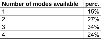
Table 3.5 presents the number of modes available by the students.The majority of the respondents have more than one mode available. So the amount of “captives” is low. The largest part of the respondents has three modes available shows that the data is very suitable for modelling the mode choice. Most of the students have something to choose.
Number of modes available perc.
1 15% 2 27% 3 34% 4 24%
3.1.2 Remarkable characteristics
The following characteristics are not the most important for the research, but are remarkable since they show some interesting characteristics of the bus and car mode.
Availability modes and corresponding choices
Table 3.6 the observed mode choices are compared with the availability of the modes. The first row contains the possible combinations of available modes and the first column contains the possible mode choices. In the table the modal split is shown per choice situation. The table shows some remarkable things. In some choice situations always one mode is preferred. Most of the times this is easy to explain by difference in cost and time: being car passenger or carpooling is less expensive than car driving or taking the bus. But in some situations when three or four modes are available, these rules apparently don’t count. When bus and car are both part of the three available modes the rules count, but when bus or car is combined with both car passenger and carpool the bus or car is suddenly preferred. The choice situation with all the modes available shows also a strange view: suddenly the car and carpool are preferred. Because the table shows contradictory things, it is hard to draw good conclusions out of it. It is a complex choice situation, where many characteristics take part in.
Table 3.6 Availability modes and observed choices
1 = car
2 = car passenger 3 = bus
4 = carpool
Differences w.r.t. gender
Table 3.7 presents the distribution in gender of the respondents that have only the bus available. The major part of them is female, which also means that male respondents have more often a car-mode available. It this case the car as driver mode shows the largest difference.
Gender perc.
Male 25% Female 75%
Table 3.7 Only bus available and gender
3.2 Modelling the mode choice
The attributes that will be taken into account in the Salerno case are presented in Table 3.8. Actually there are 11 attributes, since there is a Alternative Specific Attribute for a mode except one. As mentioned before the values of the attributes that will be used in the calibration will come out of a survey and a general supply model of the region of Campania. The values for the following attributes are taken from the supply model: Time, Access-egress time and Trip time lower than 15 minutes. The values of the other attributes are taken from the survey.
In the table the unit, the type and their relevance per mode is presented. The type of the values of the attributes is different. We can distinguish continuous, discrete and dummy. The meaning of continuous and discrete is clear. Dummy means that an attribute is given the value 0 or 1. The Alternative Specific Attributes are also dummy variables, since it gives the value 1 to one alternative and the value 0 to the others.
The dots in the table stand for which attributes are taken into account in the systematic utility of a mode.
Type Car Car passenger Bus Carpool
Level of service (LoS)
Time Trip time (h) Cont. ● ● ● ●
Cost Trip monetary cost (€) Cont. ● ● ●
Tacc-egr Access-egress time
revealed by the users (h) Cont. - - ● -
T0-15 If trip time is lower than 15
minutes - Dummy - ● - -
Socio-economic (SE)
CarAV If car mode is available - Dummy - - - ●
Gender If gender is female - Dummy - - ● -
Activity related and Land Use (LU)
ACTlength Activity time length (h) Cont. ● - - -
Freq Weekly trip frequency - Discr. - - - ●
Others
ASA - ASA ● ● - ●
3.3 Calibration and validation complete database
In this paragraph the results of the calibration and validation of the complete database of 2,808 respondents are presented. These results will be used in comparison with the results when the sample size will be changed.
Calibration
In the calibration stage the model is calibrated by changing the beta parameters until the maximum likelihood is reached. This value is: ln L(βML) = -1,932
To compare this results with the situation that the beta coefficients are all equal to 0, this value is also computed: ln L(0) = -2,505
Table 3.9 shows the beta coefficients that result after the calibration.
Beta coefficient Value
βt -1.053
Table 3.9 Beta coefficients
Indicators
The indicators in Table 3.10 show the goodness of fit of the complete database. These results can be used as a guideline by comparing the results of the same indicators at different sample sizes.
Indicators Value
Pseudo-ρ2 0.229
Fitting Factor (FF) 58.9%
Mean Square Error (MSE) 0.408 Standard Deviation (SD) 0.162
% rightCar 73.1% % rightCpas 30.5% % rightBus 75.1% % rightPool 73.1%
% right 69.7%
% clearly right (Threshold = 0.5) 61.8% % clearly wrong (Threshold = 0.5) 38.2% % unclear (Threshold = 0.5) 0.0% % clearly right (Threshold = 0.66) 39.3% % clearly wrong (Threshold = 0.66) 19.9% % unclear (Threshold = 0.66) 40.8% % clearly right (Threshold = 0.9) 17.8% % clearly wrong (Threshold = 0.9) 3.7% % unclear (Threshold = 0.9) 78.5%
Table 3.10 Indicators
4 Research method
The aim of this research is to determine the minimal sample size for calibration and hold-out. Therefore this research can be divided in two different analysis on the data:
• analysis on the calibration sample size
• analysis on the hold-out sample size
Below the take steps in both analysis are described.
Analysis on the calibration sample size
The analysis on the calibration sample size shows which amount of the real data may be considered sufficient to come to an accurate model that fits the data. The analysis on the size of a calibration sample takes several steps. First the model is calibrated by fitting the beta coefficients of the model for different sample sizes. This is done in steps of 150 interviews, starting at 150 interviews. This process was ended when after 16 different sample size 2400 interviews were taken into account in the calibration. To ensure that the results are reliable, every step is repeated 10 times with different random orders. With the results following out of the calibration of the calibration sample size the goodness of fit-indicators are calculated. So for each sample size the beta-coefficients and the goodness of fit indicators are estimated.
Sideways the remaining interviews out of every step (the hold-out sample) are used to validate the model. In this case the beta coefficients that follow from the calibration of the calibration sample size are used as fixed parameters for the calculation of the goodness of fit indicators for the hold-out sample. Since the hold-out sample size in this stage is always the remaining data from the calibration of the calibration sample, the hold-out sample size is the total of 2808 interviews minus the calibration sample size.
After these steps it is possible to see the behaviour of the beta coefficients and the goodness of fit indicators of the different calibration samples. Sideways it is possible to analyse the influence of the calibrated beta coefficients on the hold-out sample and the results of both analysis can be compared with each other.
Analysis on the hold-out sample size
After the calibration sample size is determined, this amount of data is taken away from the complete dataset. With the remaining data it is possible to determine a minimal hold-out sample.
5 Calibration sample size
In this chapter the results of the analysis on the minimal size of a calibration sample will be presented. In the first paragraph the beta coefficients that follow out of the calibration of the different sample sizes will be discussed. The second paragraph continues with the discussion of the resulting values for the goodness of fit indicators of both calibration and hold-out sample.
5.1 Beta coefficients
5.1.1 Sensitivity
A first graphical representation of the beta coefficients with a similar scale on the vertical axis shows very different results. Figure 5.11 and Figure 5.22 show this for the attributes time and cost.
17
Figure 5.1 Beta values time
-3,5
0 150 300 450 600 750 900 1050120013501500165018001950210022502400 Sample size
Figure 5.2 Beta values cost
Beta values time
-3
0 150 300 450 600 750 900 1050 1200 1350 1500 1650 1800 1950 2100 2250 2400 Sample size
The dispersion of the beta values shows big differences between the attributes. Therefore, it becomes difficult to determine the stability of each plot in a consistent way. To determine the stability in a more consistent way, the error in each beta coefficient is estimated. To determine the sensitivity of the modal split by changing the beta values the beta value of a attribute is changed while the beta values of the other attributes are fixed. When one of the mode shares shows a difference of more then 2 percent from the original share, a minimal and maximal beta value can be determined. This operation is done for all attributes and only one beta coefficients of the complete database. What results is a minimal and maximum value for the beta values and also size of the interval. All these results are presented in Table 5.1.
Attribute Final Min. Max. Size of interval Group
Time -1.053 -1.781 -0.384 1.397 C
Table 5.1 Beta values test
The table makes visible that the beta values of some attributes can differ more without changing the modal split. It is possible to group the attributes in groups on base of their size of the interval. The interval of group A is smaller than 0.2, the interval-size of the attributes in group B is between 0.2 and 1.0 and the interval of group C is bigger than 1.0.
Group A contains the following attributes:
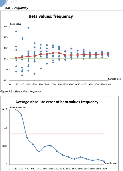
• Trip monetary cost
• Activity time length
• Frequency
These are Activity-based attributes and cost is a Level of Service attribute. The Activity-based attributes show the best performance, since the values are directly subtracted from the survey. In this survey the respondents make a choice that corresponds with the characteristics of their situation. Group B contains the following attributes:
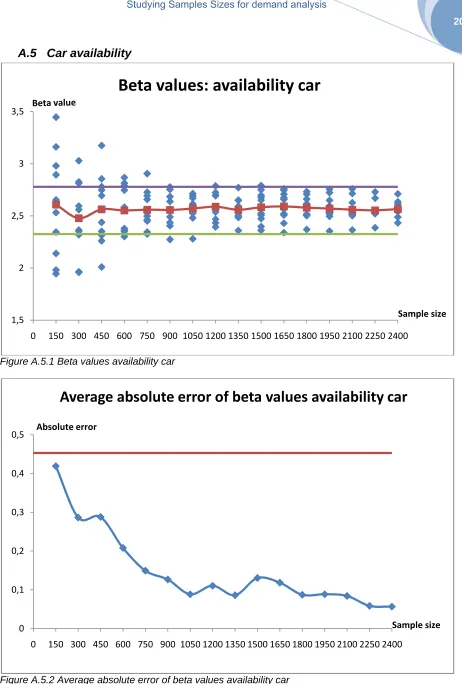
• Car availability
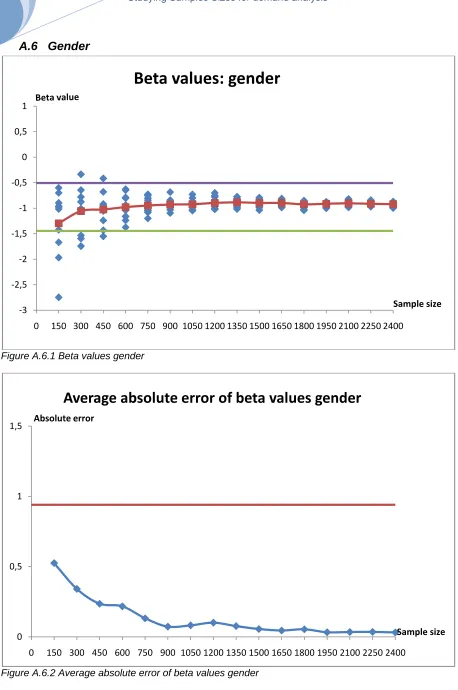
• Gender
• Alternative Specific Attributes
Car availability and gender are Socio economic attributes. The values of the Socio economic attributes come also from the survey.
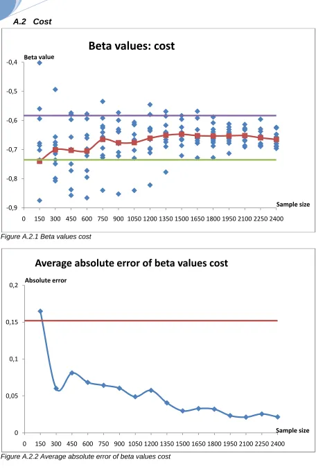
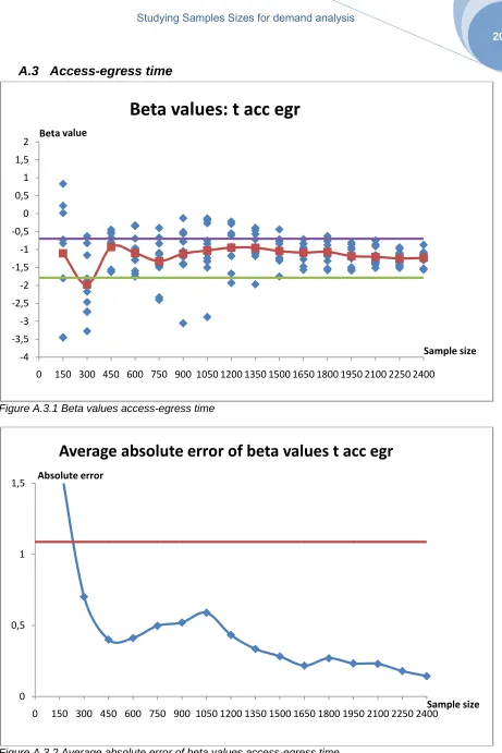
Group C contains the following attributes:
• Trip time
• Access-egress time
• Trip time lower than 15 minutes
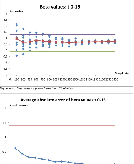
These attributes are Level of Service attributes. The values of these attributes come from the supply model of the region of Campania. The model is not capable to model the values of attributes as good as is possible with the results of the survey. The supply model is an approximation and is city based therefore. The travel time that is perceived by the users is more divided than compared to the average value of the supply model. Also for the access-egress time it estimates an average value that may be very different from that perceived by the users. Because the attribute trip time lower than 15 minutes is distracted from the attribute trip time, it has the same large interval.
5.1.2 Sample size
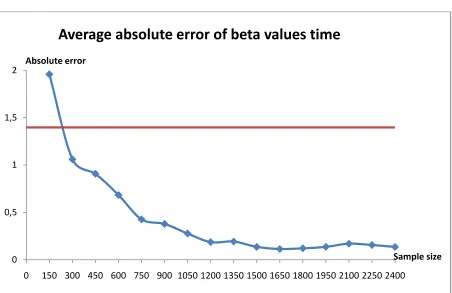
Now the sensitivity of the modal split w.r.t. changing beta values is taken into account, the stability of the graphs can be compared better. Appendix A contains graphs with all the observed beta coefficients and the average absolute error per sample size for all the attributes. An example for one of the attributes is presented in Figure 5.3 and Figure 5.4 where the beta values of the attribute time are graphed.
Figure 5.3 Beta values time
‐3,5
‐3
‐2,5
‐2
‐1,5
‐1
‐0,5 0 0,5 1 1,5
0 150 300 450 600 750 900 1050 1200 1350 1500 1650 1800 1950 2100 2250 2400
Sample size
Beta
values:
time
Figure 5.4 Average absolute error of beta values time
0 0,5 1 1,5 2
0 150 300 450 600 750 900 1050120013501500165018001950210022502400 Absolute error
Sample size
Average
absolute
error
of
beta
values
time
Beta values and average absolute error per sample size
To determine when stability of the graphs is reached, both graphs are important. The sensitivity analysis delivered an interval in which changing the beta value doesn’t change the modal split for more than 2 percent. When all the beta values are between the purple and green lines of the interval, stability is reached. Sideways the graphs of the average absolute error are also used to get a view on the behaviour of the beta values. The average absolute error is the average of the absolute difference between the average beta value and a beta value for a specific sample size.
In Table 5.2 is presented at which sample size the graphs show stable behaviour. The behaviour of the attributes still differs for the beta values and the average error, but within the attributes there is a clear relationship between the graphs. Stability is mostly reached in the same region of the graph.
Attribute Beta values Average absolute error
Time 1200 1200
Cost 1500 1500
Access-egress time 1650 1800
Trip time lower than 15 min 900 1050
Car availability 1350 1800
Gender 600 1200
Activity time length 1350 1800
Frequency 1650 1650
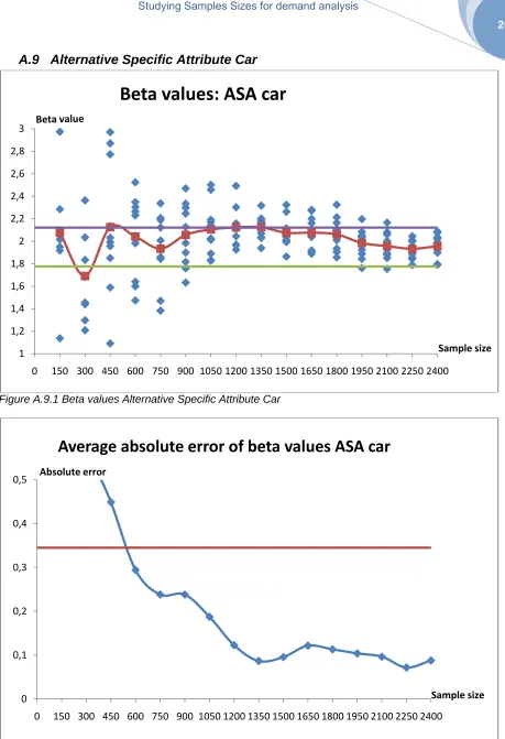
ASA Car 2250 1650
ASA Car passenger 1800 1950
ASA Carpool >2400 2400
Table 5.2 Sample sizes as stability is reached
It is complicated to summarize all the different results and come to one minimal sample size that should be sufficient to calibrate the model based on the beta values, because the sample size they become stable differs between the attributes.
5.2 Indicators
The results of the calibration and the hold-out samples can be compared with each other to determine the minimal calibration sample size. The graphs of all the indicators are presented in Appendix B. The graphs that are presented show per indicator the average per sample size and the average error per sample size.
5.2.1 Aggregate indicators
Goodness of fit statistic
To calculate this statistic the Likelihood values that follow out of the calibration/calculation can be used. The average pseudo rho-square values and the average absolute error are shown in Figure 5.5 and Figure 5.6. Because the main goal is to obtain a better insight in the minimal calibration sample size, all the results in the graphs are presented with respect to the calibration sample size. By reviewing the graphs to determine the minimal sample size should be taken into account that the larger the amount of interviews becomes, the larger becomes also the dependence between the different samples. It can be expected that the graphs show that the results become more and more the same, because the overlap of the used data becomes larger. But when the results reach the same value before the maximum of the dataset is reached, this indicates a sufficient sample size can be determined. Of course it is difficult to call a graph stable when the values become almost the same. In this research there are no tools used to calculate the stability of the graphs, but the stability of the graphs is just viewed on the eye.
Besides the behaviour of the graphs that is described above, the graphs of the hold-out sample will show a different behaviour. This is because the calibration size increases and the hold-out sample decreases. At the beginning the behaviour of the indicators w.r.t. the hold-out sample will be unstable because the hold-out sample is calculated with results of a small calibration sample size. At the end the hold-out sample the behaviour of the indicators w.r.t. the hold-out sample will also be unstable because the hold-out sample is small.
The graph shown stable behaviour after 1350 interviews. The graph of the hold out sample confirms this, because this graph also becomes stable at this point.
21
Figure 5.5 Average pseudo rho-square value
Average pseudo rho-square value
0.2
0 150 300 450 600 750 900 1050 1200 1350 1500 1650 1800 1950 2100 2250 2400
Calibration sample size Pseudo rho-square
value
Average absolute error of pseudo rho-square value
0 0.01 0.02 0.03 0.04 0.05
0 150 300 450 600 750 900 1050 1200 1350 1500 1650 1800 1950 2100 2250 2400
Calibration sample size Absolute error
Hold-out Calibration
Figure 5.6 Average absolute error of pseudo rho-square value
Fitting factor
The graph of the fitting factor in Figure 5.7 also become stable at a calibration sample size of 1350. It is remarkable that the hold-out sample almost reach the same fitting factor.
Average Fitting factor (FF)
58% 59% 60% 61% 62% 63%
0 150 300 450 600 750 900 1050 1200 1350 1500 1650 1800 1950 2100 2250 2400
Calibration sample size FF
Calibration
Hold-out
Figure 5.7 Average Fitting Factor
Mean Square Error(MSE) and Standard Deviation(SD)
5.2.2 Clearness analysis
% right
This statistic not only reaches stability for both the calibration and hold-out sample but also reaches almost the same value after 1350 interviews. Figure 5.8 shows the average. The indicator varies among a very small interval.
This statistic can also be graphed per mode, but it is complicated to make remarks on the graphs of the specific travel modes. The graphs do not show the expected behaviour and the graphs of the average value become stable almost at the end of the process. This indicator is not an effective attribute to compare models. In this case the process can be stopped after 300 observations.
Average % right
65%
0 150 300 450 600 750 900 1050 1200 1350 1500 1650 1800 1950 2100 2250 2400
Calibration sample size
% right
Calibration Hold-out
Figure 5.8 Average % right
% clear
There is a small trend visible, but it is not for every graph possible to distinguish a good point where the graph become stable. In Figure 5.9 are two examples shown where it is possible to determine the minimal calibration sample size. After 1350 interviews the graphs give a better stable view.
Average % clearly right t=0,66
38%
0 150 300 450 600 750 900 1050 1200 1350 1500 1650 1800 1950 2100 2250 2400
Calibration sample size % clearly right
Calibration Hold-out
Figure 5.9 Average % clearly right threshold=0.66
5.2.3 Minimal calibration sample size
Although it is hard to distinguish at which calibration sample size the graphs become stable and some indicators have more importance than others, it is possible to estimate these points. In Table 5.3 the results of this estimation are shown.
Indicator
Calibration sample Hold-out sample Average Average
absolute error
Average Average absolute error
ρ2 1350 1200 1350 900
% clearly right
threshold =0.5 1350 1350 1200 1050
% clearly wrong
threshold =0.5 1350 1350 1200 1050
% clearly right
threshold =0.66 1350 1350 600 1350
% clearly wrong
threshold =0.66 600 1350 750 900
% unclear
threshold =0.66 750 1800 750 1350
% clearly right
threshold =0.9 1350 1050 600 900
% clearly wrong
threshold =0.9 600 600 600 600
% unclear threshold =0.9
1350 1350 1500 900
Table 5.3 Minimal calibration sample size
The table also shows a diffuse view, but most of the graphed indicators reach stability around 1350 interviews. Between the different graphs of an indicator, there is of course a correlation. Mostly the graphs of the same indicator reach stability in the same range of interviews.
6 Hold-out sample size
The analysis of the minimal hold-out sample needs a different approach then the analysis on the minimal calibration sample. The analysis on the calibration sample size should happen before the analysis on the hold-out sample, because the minimal calibration sample size will be taken out and the beta values of the calibration of this sample will be used as fixed parameters for the calculation of the model with the hold-out sample. In the first paragraph the differences between the observed choices and the modelled choices, that follow out of the calculation of the model, will be presented. The second paragraph will discuss the different results w.r.t. the indicators.
6.1 Indicators
6.1.1 Aggregate indicators
Goodness of fit statistic
Figure 6.1 and Figure 6.2 shows the graph of the average pseudo rho-square value and the average absolute error of the rho-square value. The graph of the average value shows that it becomes stable after 800 interviews. The graph of the average absolute error does not indicate stable behaviour before the maximum sample size is reached. The graph is stable in the sense that it approaches zero in almost equal steps, but for the analysis on the minimal hold-out sample size this not sufficient, because it should reach a constant value before the maximum sample size is reached. All the graphs of the average absolute error of the indicators cannot give a good sample size where a stable value is reached, so the graph of the average absolute error would not be displayed anymore. But all these graphs are displayed in appendix C.
Average pseudo rho-square value
0.20 0.21 0.22 0.23 0.24 0.25
0 100 200 300 400 500 600 700 800 900 1000 1100 1200 1300
Sample size Pseudo
Rho-square value
Figure 6.1 Average Pseudo rho-square value
Average absolute error of pseudo rho-square value
0 0.005 0.01 0.015 0.02 0.025 0.03 0.035 0.04 0.045 0.05
0 100 200 300 400 500 600 700 800 900 1000 1100 1200 1300
Sample size Absolute error
Figure 6.2 Average absolute error of pseudo rho-square value
Fitting factor
Out of Figure 6.3 with the average fitting factor also comes clear that the minimal hold-out sample sizes is reached after 800 interviews, although the differences are small.
Average Fitting factor (FF)
55% 56% 57% 58% 59% 60%
0 100 200 300 400 500 600 700 800 900 1000 1100 1200 1300
Sample size FF
Figure 6.3 Average Fitting Factor
Mean Square Error(MSE) and Standard Deviation(SD)
6.1.2 Clearness analysis
% right
Also for the graph of the average % right in Figure 6.4 the differences are small, but after 800 interviews the difference with the values of other sample sizes is decreased.
Average % right
65%
0 100 200 300 400 500 600 700 800 900 1000 1100 1200 1300
Sample size % right
Figure 6.4 Average % right
% clear
Figure 6.5, where the average % clearly right with a threshold of 0.66 is graphed, gives a better view on a which hold-out sample size stability is reached. It is obvious that the graph does not change after 800 interviews. Although this graph gives a clear view, not all the graphs of the clearly analysis are as clear as this.
Average % clearly right t=0,66
36%
0 100 200 300 400 500 600 700 800 900 1000 1100 1200 1300
Sample size % clearly right
Figure 6.5 Average % clearly right threshold=0.66
6.2 Minimal hold-out sample size
Although it is not easy to distinguish at which hold-out sample size the graphs become stable and some indicators have more importance than others, it is possible to estimate these points. In Table 6.1 the results of this estimation are shown.
Indicator Average Average absolute error
ρ2 800 800
FF 800 1000
MSE 800 1000
SD 800 800
% right car 700
-% right pas 900 800
% right bus 800 900
% right pool 700
-% right 800
-% clearly right threshold =0.5 700 1000
% clearly wrong threshold =0.5 700 1000
% clearly right threshold =0.66 800
-% clearly wrong threshold =0.66 1000 1000
% unclear threshold =0.66 1100
-% clearly right threshold =0.9 800 1000
% clearly wrong threshold =0.9 800 900
% unclear threshold =0.9 700
-Table 6.1 Minimal hold-out sample size
7 Conclusions and recommendations
In this report the calibration and hold-out sample size have been analysed. The main goal was to estimate/determine the minimal sample size. This has been done with a very simple approach, the size of both samples has been obtained by progressively increasing the number of observations, randomly sampled out of the available Salerno database. The results of the calibrated and calculated models are evaluated with several indicators.
Although not all the results were even clear, it was possible to determine both minimal sample sizes. The minimal sample size to calibrate a model with the same characteristics as the Salerno case should be 1500 observations. The minimal hold-out sample size to control the outcomes of the model should be 800 observations.
In this research only the MultiNomial Logit Model is used, but the minimal sample size for other models is still an open issue. This research on the MultiNomial Logit Model can be used as a benchmark model. Also it is useful to evaluate the indicators that will be used after such an analysis, because with the MultiNomial Logit Model some indicators do not give clear results or results similar to others.
Another issue that can be further analysed to give the results of this analysis more importance is the behaviour of the beta values and the values of the attributes in the systematic utility. It seems that there is a big difference in sensitivity on the modal split between the attributes. In addition to the sensitivity analysis on the attributes it seems also useful to carry out a preliminary analysis on the relevance of attributes.
To control the results of this analysis on the Salerno case the proposed approach should also be applied on a different case with the same characteristics as the Salerno case, because the Salerno case is a specific case with his own characteristics.
8 References
• Cantarella, G.E., De Luca, S. (2002), Modelling mode choice behaviour for intercity journeys, Proceedings of the European Transport Conference, University of Cambridge, United
Kingdom
• Cantarella, G.E., De Luca, S. (2007) Validation and comparison of choice models
[forthcoming]
• Cantarella, G.E., Fedele, V., (2003), Fuzzy vs. random utility models: an application to mode
choice behaviour analysis, Proceedings of European Transport Conference, Strasbourg,
France
• Cascetta, E. (2001), Transportation Systems Engineering: theory and methods, Kluwer Academic Publishers, Dordrecht, The Netherlands
• Steehouder, M. e.a. (1992). Leren Communiceren, Wolters-Noordhoff, Groningen, The
Appendices
A Beta coefficients Analysis Calibration sample size ... 1
A.1 Time ... 1
A.2 Cost ... 2
A.3 Access-egress time ... 3
A.4 Trip time lower than 15 minutes ... 4
A.5 Car availability ... 5
A.6 Gender ... 6
A.7 Activity time length ... 7
A.8 Frequency ... 8
A.9 Alternative Specific Attribute Car ... 9
A.10 Alternative Specific Attribute Car passenger ... 10
A.11 Alternative Specific Attribute Carpool ... 11
B Indicators Analysis Calibration sample size ... 12
B.1 Aggregate indicators ... 12
B.2 Clearness analysis ... 16
C Indicators Analysis Hold out sample size ... 29
C.1 Aggregate indicators ... 29
A Beta
coefficients
Analysis Calibration sample size
A.1 Time
Figure A.1.1 Beta values time
‐3,5
‐3
‐2,5
‐2
‐1,5
‐1
‐0,5 0 0,5 1 1,5
0 150 300 450 600 750 900 1050 1200 1350 1500 1650 1800 1950 2100 2250 2400
Sample size
Beta
values:
time
0 0,5 1 1,5 2
0 150 300 450 600 750 900 1050 1200 1350 1500 1650 1800 1950 2100 2250 2400
Absolute error
Sample size
A.2 Cost
2 Figure A.2.1 Beta values cost
‐0,9
‐0,8
‐0,7
‐0,6
‐0,5
‐0,4
0 150 300 450 600 750 900 1050 1200 1350 1500 1650 1800 1950 2100 2250 2400
Sample size
Beta
values:
cost
Figure A.2.2 Average absolute error of beta values cost
0 0,05 0,1 0,15 0,2
0 150 300 450 600 750 900 1050 1200 1350 1500 1650 1800 1950 2100 2250 2400
Absolute error
Sample size
A.3 Access-egress
time
Figure A.3.1 Beta values access-egress time
‐4
‐3,5
‐3
‐2,5
‐2
‐1,5
‐1
‐0,5 0 0,5 1 1,5 2
0 150 300 450 600 750 900 1050 1200 1350 1500 1650 1800 1950 2100 2250 2400
Sample size
Beta
values:
t
acc
egr
Figure A.3.2 Average absolute error of beta values access-egress time
0 0,5 1 1,5
0 150 300 450 600 750 900 1050 1200 1350 1500 1650 1800 1950 2100 2250 2400
Absolute error
Sample size
A.4 Trip time lower than 15 minutes
4 Figure A.4.1 Beta values trip time lower than 15 minutes
‐2
‐1,5
‐1
‐0,5 0 0,5 1 1,5 2 2,5 3
0 150 300 450 600 750 900 1050 1200 1350 1500 1650 1800 1950 2100 2250 2400
Sample size
Beta
values:
t
0
‐
15
Figure A.4.2 Average absolute error of beta values trip time lower than 15 minutes
0 0,5 1 1,5 2
0 150 300 450 600 750 900 1050 1200 1350 1500 1650 1800 1950 2100 2250 2400
Absolute error
Sample size
A.5 Car
availability
Figure A.5.1 Beta values availability car
1,5 2 2,5 3 3,5
0 150 300 450 600 750 900 1050 1200 1350 1500 1650 1800 1950 2100 2250 2400
Sample size
Beta
values:
availability
car
Figure A.5.2 Average absolute error of beta values availability car
0 0,1 0,2 0,3 0,4 0,5
0 150 300 450 600 750 900 1050 1200 1350 1500 1650 1800 1950 2100 2250 2400
Absolute error
Sample size
A.6 Gender
6 Figure A.6.1 Beta values gender
‐3
‐2,5
‐2
‐1,5
‐1
‐0,5 0 0,5 1
0 150 300 450 600 750 900 1050 1200 1350 1500 1650 1800 1950 2100 2250 2400
Sample size
Beta
values:
gender
Figure A.6.2 Average absolute error of beta values gender
0 0,5 1 1,5
0 150 300 450 600 750 900 1050 1200 1350 1500 1650 1800 1950 2100 2250 2400
Absolute error
Sample size
A.7 Activity time length
Figure A.7.1 Beta values activity time length
‐0,4
‐0,3
‐0,2
‐0,1 0 0,1
0 150 300 450 600 750 900 1050 1200 1350 1500 1650 1800 1950 2100 2250 2400
Sample size
Beta
values:
ACT
length
Figure A.7.2 Average absolute error of beta values activity time length
0 0,05 0,1 0,15
0 150 300 450 600 750 900 1050 1200 1350 1500 1650 1800 1950 2100 2250 2400
Absolute error
Sample size
A.8 Frequency
8 Figure A.8.1 Beta values frequency
‐0,1 0 0,1 0,2 0,3 0,4
0 150 300 450 600 750 900 1050 1200 1350 1500 1650 1800 1950 2100 2250 2400
Sample size
Beta
values:
frequency
Figure A.8.2 Average absolute error of beta values frequency
0 0,05 0,1 0,15
0 150 300 450 600 750 900 1050 1200 1350 1500 1650 1800 1950 2100 2250 2400
Absolute error
Sample size
A.9 Alternative
Specific Attribute Car
Figure A.9.1 Beta values Alternative Specific Attribute Car
1 1,2 1,4 1,6 1,8 2 2,2 2,4 2,6 2,8 3
0 150 300 450 600 750 900 1050 1200 1350 1500 1650 1800 1950 2100 2250 2400
Sample size
Beta
values:
ASA
car
Figure A.9.2 Average absolute error of beta values Alternative Specific Attribute Car
0 0,1 0,2 0,3 0,4 0,5
0 150 300 450 600 750 900 1050 1200 1350 1500 1650 1800 1950 2100 2250 2400
Absolute error
Sample size
A.10 Alternative Specific Attribute Car passenger
10 Figure A.10.1 Beta values Alternative Specific Attribute car passenger
‐5
‐4,5
‐4
‐3,5
‐3
‐2,5
‐2
‐1,5
‐1
0 150 300 450 600 750 900 1050 1200 1350 1500 1650 1800 1950 2100 2250 2400
Sample size
Beta
values:
ASA
carpassenger
Figure A.10.2 Average absolute error of beta values Alternative Specific Attribute car passenger
0 0,1 0,2 0,3 0,4 0,5 0,6 0,7 0,8 0,9 1
0 150 300 450 600 750 900 1050 1200 1350 1500 1650 1800 1950 2100 2250 2400
Absolute error
Sample size
Average
absolute
error
of
beta
values
ASA
car
A.11 Alternative Specific Attribute Carpool
Figure A.11.1 Beta values Alternative Specific Attribute carpool
‐3,5
‐3,3
‐3,1
‐2,9
‐2,7
‐2,5
‐2,3
‐2,1
‐1,9
‐1,7
‐1,5
0 150 300 450 600 750 900 1050 1200 1350 1500 1650 1800 1950 2100 2250 2400
Sample size
Beta
values:
ASA
carpool
Figure A.11.2 Average absolute error of beta values Alternative Specific Attribute carpool
0 0,1 0,2 0,3 0,4 0,5
0 150 300 450 600 750 900 1050 1200 1350 1500 1650 1800 1950 2100 2250 2400
Absolute error
Sample size
B Indicators Analysis Calibration sample size
1.1 Aggregate
indicators
12 Figure B.1.1 Average pseudo rho-square value
Average pseudo rho-square value
0.2 0.21 0.22 0.23 0.24 0.25
0 150 300 450 600 750 900 1050 1200 1350 1500 1650 1800 1950 2100 2250 2400
Calibration sample size Pseudo rho-square
value
Hold-out Calibration
Average absolute error of pseudo rho-square value
0 0.01 0.02 0.03 0.04 0.05
0 150 300 450 600 750 900 1050 1200 1350 1500 1650 1800 1950 2100 2250 2400
Calibration sample size Absolute error
Hold-out Calibration
Average Fitting factor (FF)
58% 59% 60% 61% 62% 63%
0 150 300 450 600 750 900 1050 1200 1350 1500 1650 1800 1950 2100 2250 2400
Calibration sample size FF
Calibration
Hold-out
Figure B.1.3 Average Fitting Factor
Average Absolute error Fitting factor
0% 1% 2% 3% 4% 5%
0 150 300 450 600 750 900 1050 1200 1350 1500 1650 1800 1950 2100 2250 2400
Calibration sample size Absolute error
Calibration Hold-out
Average Mean Square Error (MSE)
0.38 0.39 0.40 0.41 0.42 0.43
0 150 300 450 600 750 900 1050 1200 1350 1500 1650 1800 1950 2100 2250 2400
Calibration sample size MSE
Calibration
Hold-out
Figure B.1.5 Average Mean Square Error
Average Absolute error Mean Square Error (MSE)
0.00 0.01 0.02 0.03 0.04 0.05
0 150 300 450 600 750 900 1050 1200 1350 1500 1650 1800 1950 2100 2250 2400
Calibration sample size Absolute error
Calibration Hold-out
Figure B.1.6 Average Absolute error Mean Square Error
Average Standard Deviation(SD) of Mean Square Error
0.15 0.16 0.17 0.18 0.19 0.20
0 150 300 450 600 750 900 1050 1200 1350 1500 1650 1800 1950 2100 2250 2400
Calibration sample size SD
Calibration Hold-out
Figure B.1.7 Average Standard Deviation of Mean Square Error
Average Absolute error of Standard Deviation (SD)
0.00 0.01 0.02 0.03 0.04 0.05
0 150 300 450 600 750 900 1050 1200 1350 1500 1650 1800 1950 2100 2250 2400
Calibration sample size Absolute error
Calibration
Hold-out
B.2 Clearness
analysis
Average % right
65%
0 150 300 450 600 750 900 1050 1200 1350 1500 1650 1800 1950 2100 2250 2400
Calibration sample size
% right
Calibration Hold-out
Figure B.2.1 Average % right
Average Absolute error % right
0%
0 150 300 450 600 750 900 1050 1200 1350 1500 1650 1800 1950 2100 2250 2400
Calibration sample size Absolute error
Calibration
Hold-out
Figure B.2.2 Average absolute error % right
Average % right car
Calibration sample size % right
Calibration Hold-out
Figure B.2.3 Average % right car
Average Absolute error % right car
0%
0 150 300 450 600 750 900 1050 1200 1350 1500 1650 1800 1950 2100 2250 2400
Calibration sample size
Absolute error
Calibration
Hold-out
Average % right carpassenger
0 150 300 450 600 750 900 1050 1200 1350 1500 1650 1800 1950 2100 2250 2400
Calibration sample size % right
Calibration
Hold-out
Figure B.2.5 Average % right car passenger
Average Absolute error % right carpassenger
0%
0 150 300 450 600 750 900 1050 1200 1350 1500 1650 1800 1950 2100 2250 2400
Calibration sample size
Absolute error
Calibration
Hold-out
Figure B.2.6 Average absolute error % right car passenger
Average % right bus
0 150 300 450 600 750 900 1050 1200 1350 1500 1650 1800 1950 2100 2250 2400
Calibration sample size % right
Calibration Hold-out
Figure B.2.7 Average % right bus
Average Absolute error % right bus
0%
0 150 300 450 600 750 900 1050 1200 1350 1500 1650 1800 1950 2100 2250 2400
Calibration sample size Absolute error
Calibration Hold-out
Average % right carpool
0 150 300 450 600 750 900 1050 1200 1350 1500 1650 1800 1950 2100 2250 2400
Calibration sample size % right
Calibration
Hold-out
Figure B.2.9 Average % right carpool
Average Absolute error % right carpool
0%
0 150 300 450 600 750 900 1050 1200 1350 1500 1650 1800 1950 2100 2250 2400
Calibration sample size
Absolute error
Calibration Hold-out
Figure B.2.10 Average absolute error % right carpool
Average % clearly right t=0,5
60% 61% 62% 63% 64% 65%
0 150 300 450 600 750 900 1050 1200 1350 1500 1650 1800 1950 2100 2250 2400
Calibration sample size
% clearly right
Calibration Hold-out
Figure B.2.11 Average % clearly right threshold=0.5
Average Absolute error % clearly right t=0,5
0% 1% 2% 3% 4% 5%
0 150 300 450 600 750 900 1050 1200 1350 1500 1650 1800 1950 2100 2250 2400
Calibration sample size Absolute error
Calibration Hold-out
Average % clearly right t=0,66
38% 39% 40% 41% 42% 43%
0 150 300 450 600 750 900 1050 1200 1350 1500 1650 1800 1950 2100 2250 2400
Calibration sample size
% clearly right
Calibration Hold-out
Figure B.2.13 Average % clearly right threshold=0.66
Average Absolute error % clearly right t=0,66
0% 1% 2% 3% 4% 5%
0 150 300 450 600 750 900 1050 1200 1350 1500 1650 1800 1950 2100 2250 2400
Calibration sample size Absolute error
Calibration
Hold-out
Figure B.2.14 Average absolute error % clearly right threshold=0.66
Average % clearly right t=0,9
17% 18% 19% 20% 21% 22%
0 150 300 450 600 750 900 1050 1200 1350 1500 1650 1800 1950 2100 2250 2400
Calibration sample size
% clearly right
Calibration Hold-out
Figure B.2.15 Average % clearly right threshold=0.9
Average Absolute error % clearly right t=0,9
0% 1% 2% 3% 4% 5%
0 150 300 450 600 750 900 1050 1200 1350 1500 1650 1800 1950 2100 2250 2400
Calibration sample size Absolute error
Calibration Hold-out
Average % clearly wrong t=0,5
35% 36% 37% 38% 39% 40%
0 150 300 450 600 750 900 1050 1200 1350 1500 1650 1800 1950 2100 2250 2400
Calibration sample size % clearly wrong
Calibration Hold-out
Figure B.2.17 Average % clearly wrong threshold=0.5
Average Absolute error % clearly wrong t=0,5
0% 1% 2% 3% 4% 5%
0 150 300 450 600 750 900 1050 1200 1350 1500 1650 1800 1950 2100 2250 2400
Calibration sample size Absolute error
Calibration Hold-out
Figure B.2.18 Average absolute error % clearly wrong threshold=0.5
Average % clearly wrong t=0,66
18% 19% 20% 21% 22% 23%
0 150 300 450 600 750 900 1050 1200 1350 1500 1650 18