Facial rendering

F

ACIAL

RENDERING

. . . .

. . . .

Master thesis

A

:

N. A. Nijdam

S

:

. . . .

. . . .

P

REFACE

This document describes my graduation on the University of Twente, Human Media Interaction division. This document is intended for those who are interested in the development and use of virtual environments created with the use of OpenGL and the rendering procedure for facial representation.

The Human Media Interaction(HMI) division is part of the "Electrical Engineering", "Mathematics" and "Computer Science" division at the University of Twente. HMI is all about the interaction between human and machine and offers a great range of topics. One of those topics is Virtual Reality & Graphics which is a very broad topic in itself. The graduation project falls within this topic with the emphasis on graphics. The project is based on work of The Duy Bui[12], where a virtual head model has been developed for facial expressions using an underlying muscle system, and aims at visually improving the head model. Related work in this field are skin rendering, realistic lighting, organic material rendering, shadowing, shader programming and advanced rendering techniques.

N. A. Nijdam

. . . .

. . . .

C

ONTENTS

1 Introduction . . . .1

Chapter overview 2

2 Lighting models . . . .5

2.1 Default OpenGL lighting . . . 5

Emission 7 Ambient 7 Diffuse 7 Specular 7 Attenuation 8 Blinn-phong shading calculation 8

2.2 Cook-Torrance . . . 9

2.3 Oren-Nayar . . . 9

2.4 Environment mapping . . . 10

Sphere mapping 10 Cube mapping 13 Paraboloid mapping 14

2.5 Environment map as Ambient light . . . 15

2.6 Spherical harmonics. . . 15

The definition 15 Projection 16

2.7 Lighting and texturing. . . 18

2.8 Conclusion . . . 19

3 Bump mapping. . . .21

3.1 the normal vector . . . 21

Normal vector per polygon 21 Normal vector per vertex 21 Normal vector per fragment 22

3.2 Light the bumps using normal maps . . . 22

Normal maps and object space 22 Normal maps and tangent space 23

3.3 Creating a normal map. . . 25

3.4 Parallax mapping . . . 26

4 Real-time shadow casting. . . .29

4.1 Shadow mapping . . . 29

4.2 Soft shadows using shadow mapping . . . 32

5 Deferred shading . . . .35

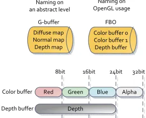
5.1 The layout of the buffers . . . 35

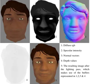
5.2 Material pass . . . 36

5.3 Lighting pass . . . 38

CONTENTS

5.5 Conclusion . . . 42

6 Facial rendering . . . .43

6.1 The HMI face model . . . 43

The Face mesh 43 Muscle system 44 The conversion 44

6.2 Rendering the skin . . . 44

Basic skin rendering 45 Diffuse mapping 45 Bump mapping 45 Specular mapping 47

6.3 Rendering the eyebrow . . . 48

The blend function 48 The eyebrow mesh 48 Parameters vertex offset and alpha blending 49 Final result 50

6.4 Rendering the eyes . . . 50

6.5 Rendering the Eyelashes . . . 52

7 Conclusion . . . .55

8 Future work . . . .59

Bibliography . . . .61

Appendices . . . .65

A The OpenGL render pipeline . . . .67

A.1 Overview . . . 67

OpenGL Geometric primitives 68 3D models 68 Coordinate spaces 69

A.2 OpenGL buffers . . . 71

Color buffers 72

Depth buffer 72

Stencil buffer 73

Accumulation buffer 73

. . . .

. . . .

A

BSTRACT

Based on the work of the TheDuy Buy the primary goal is increasing the visual realism of the virtual head model in a real-time environment. Especially the area around the eyes. In order to do so, several aspects of the head are taken apart and handled separatly.

The skin is updated by using multiple textures for the base color, specular intensity and normal maps providing skin color and skin imperfections. Using a different lightmodel then the default per vertex lighting OpenGL model, a more realistic lighting environment is created reflecting the skin more realistic. The lighting model constists of three parts: ambient lighting using Spherical harmonics, diffuse lighting using Oren-Nayar model and specular lighting using the Cook-Torrance model. In combination with bumpmapping (using the normal maps) a very detailed skin surface is constructed.

The eyebrows are replaced with a texture based patch, providing a more customizable eyebrow. A specialised shader (fur shader) is written in order make the eyebrow appear more voluminous.

The eyelashes are replaced with a more modular and generic approach. Where the original model uses hardcoded nodes, the new model uses a freely movable bouding box which provides the place where the eyelash is created (using the vertices within the bounding box).

The eyes are separated into two parts: the eyeball and the iris. The iris uses a specialised shader, providing the eye visually with sublte effects like a lens distortion effect, a reflective spot on the outside of the iris, an inside illumination on the iris and an environment reflection stretched over the eye.

The head is provided with a self-shadowing technique called shadowmapping. Extended with a softshadowing algorithm, subtle lighting effects are created on the face. Improving the way light affects the head.

. . . .

. . . .

1

I

NTRODUCTION

ecent developments in Human Computer Interaction (HCI) try to incorporate Virtual Reality (VR) techniques in situations where human-human interactions as well as human-computer interactions are important. For instance, human avatars can represent participants within a meeting situation where the real person cannot be physically present. In health care, an avatar might provide information and instructions to patients, or talk to elderly persons. In most situations, it is required that the avatar is, at the very least, a “believable” human. Such avatars should look reasonably realistic. Moreover, they should be able to show human-like facial expressions and emotions, and should show appropriate body language, including gaze behaviour. The use of graphics can give a certain visual impression for a virtual environment. The focus on graphics can be to make a virtual reality as realistic as possible or a more simplified approach with a cartoon style rendering. This is dependent on how the most important aspects of graphics, which are lighting and materials, are simulated. The use of graphics in a real time virtual reality is dependent on current hardware capabilities and software technologies. Graphical technologies which were only possible in the past by non-realtime rendering can now be performed in real time. This offers new possibilities to implement new visual presentations for virtual reality which have the requirement to be performed in real-time.

In this master’s thesis, we focus on one aspect: the visual appearance of the human face, and, more in particular, the area around the eyes. A second goal was to improve substantially the applicability and reusability of a software model based upon Parke & Water’s original head model, later on further developped by The Duy Buy.

•

•

The head model from The Duy Bui uses the default OpenGL lighting (per vertex Phong-Blinn based lighting model) and has no support for texturing. The head appearance is based on a single skin color and uses a constant reflective intensity over the whole face. The per vertex based lighting model doesn't support subtle facial irregularities. This clearly doesn't look realistic. Facial irregularities are important as it defines the look of a face of a person. It shows age and imperfections of the face such as scars and birthmarks which gives an impression of the character and makes it unique. In order to support these aspects a per fragment based lighting model is used. With today's hardware shader capabilities this is easily done in real-time and can support complex lighting models in real-time. With more accurate material properties the skin can be simulated more realistically, instead of using a single color on the face. This directly involves the use of textures, which can improve the appearance of the head model by using an image providing the color information on the model. The use of textures in real-time isn't new, however, the use of textures and hardware shader capabilities give a new dimensions on how to use these textures.

INTRODUCTION

1

Usually a texture is a two dimensional array where each entry contains a color. Using a texture to lookup the color for a specific fragment is its main purpose, but textures can be used to store all kinds of information and can be utilized in shader programs as inputs for an algorithm (such as a lighting model). A basic lighting approach is to calculate the light reflective intensity. This is usually done by a dot product of the normal vector (the normalized perpendicular vector on the surface of an object) and the light vector (the normalized vector pointing from the surface of an object towards the light source). The normal vector usually is calculated by a planar equation from the polygon, but can be manipulated. The manipulation of this vector can create the impression of bumps (so called bump mapping) and can be further extended to create facial irregularities such as wrinkles. These manipulated normals can be stored in the textures. Another use for textures is to store the specular intensity. This is useful for the face in order to make certain areas on the face more reflective. This for example is the case with the nose area which in contrast to the cheeks is more reflective. Also if sweating a lot the forehead will appear more shiny then most parts of the face. A texture can incorporate these informations at a per fragment level, and can easily be read by a shader program. This offers new possibilities on how to use the head model and on how we want to present a model.

As the eyebrow is part of the face it is taken into account on how we perceive a person ( as we directly create an opinion based on looks). They are used to complement facial expressions such as frown or just raising one eyebrow. By making these more realistic it can raise the acceptance of the person and the possible expressions. The head model from The Duy Bui offers a very basic eyebrow represented by a small arc stripe with a single color. In order to make this more realistic the single stripe is replaced by a texture based eyebrow, combined with a custom designed shader program (a so called fur shader) to create a more voluminous eyebrow.

The eyes from the head model use a low quality texture containing the iris color information, and also a static light reflection spot. Using a low resolution texture can give a good result on a small object or at a greater distance, however when only rendering the face, the details of the eye are more evident. Therefore a higher resolution texture capable of containing a more detailed iris is used, which can be from a real source (such as a photo) or custom generated. The static light reflection spot gives the impression of a light source reflecting in the eye, but this can be easily done in real time by the light model. By providing the eyes with a high reflective intensity the light model can take the actual light sources in the scene to provide accurate reflection highlights in the eye. This in order to provide additional cues on how the light is affecting the head model and making it more realistic. Another aspect of light is the creation of shadows. Shadows provide additional cues on how the light is distributed over the face. A shadowing technique called shadow mapping is therefore implemented.

A minor part of the eyes are the eyelashes which are provided by a static eyelash model. Replacing this model with a more custom designed eyelashes using an external texture gives the possibility to create new eyelashes more easily and more realistic eyelashes can be provided.

Where most research papers discuss one technique, here a full scale of methods is presented and described on how they can be used together. The rest of this chapter gives a more detailed introduction/overview on the project. The first 5 chapters introduce the several rendering techniques and its uses and in chapter 6 the techniques are used on the head model.

C h a p t e r o v e r v i e w

INTRODUCTION

of this model certain key areas are defined: lighting, materials and special effects. The lighting is basically the most important aspect of visualizing the head model, the material gives structure to the surface of the head model and the special effects can add certain modifications to the final image before it is presented on screen. The interaction between the lighting and the way materials are handled is very close, and is incorporated in a so called lighting model or bidirectional reflectance distribution function model (BRDF). The lighting in a virtual environment is an approach for real-world lighting using a mathematical algorithm calculating the "correct" color at each pixel. The material information is used as attributes for regulating the algorithm, which can be done by setting the reflective colors or special function parameters (such as a Fresnel factor used by certain BDRF models). Setting the “correct” color at each pixel is done by combining certain colors based on the lighting aspects. This can be very basic or very complex. In the system from The Duy Bui a most simplistic diffuse color is used, which defines only one color to be used as the diffuse reflection color for a part of the face. To make this more complex, lighting can be separated into multiple components, ambient, diffuse and specular, where for each component a color can be assigned. Still this is on a complete region and to create more detail the use of surface color maps are used, which contain the color information to be used at any part of the face. This is also called texturing. This approach can be further extended by multi-texturing (using multiple color maps as layers over each other) where the way of combining the textures is also defined by a algorithm. The color maps are used for the diffuse component. The way the diffuse is handled can be replaced by other models. OpenGL default is the Lambertian diffuse model which is used by the Blinn-Phong shading model. Here another well known model is presented, the Oren-Nayar reflection model and is used to replace the default diffuse lighting model. This diffuse model simulates rough surface features, which scatter light more unevenly then the Lambertion diffuse model, and makes it ideal for a skin surface. The other components can also be extended with a variety of techniques. The ambient component can be one color, or a more complex model. For example a low frequency light model, based on a so called spherical harmonics, can be used. Another method is a real-time environmental ambient illumination, by taking the colors around the object as an ambient input (environment mapping). The last component of the lighting model , called “specular lighting”, is used to show highlights and is presented here with the Blinn-Phong model and the Cook-Torrance model.

Chapter 3 “Bump mapping” introduces a technique for modulating the lighting at a per fragment level in order to simulate bumps which can be used to simulate wrinkles and skin irregularities.

Chapter 4 “Real-time shadow casting” handles the self-shadowing. Although it may seem to be a part of the lighting model, shadowing is a complete separate subject. With lighting calculations one specific point (vertex or fragment) is processed at a time and for that point in solitude a lighting calculation is performed using only the point information and the lighting information. However this doesn't include concepts like occlusion. If the light ray is intercepted by an object standing in front of the point being illuminated a specialized algorithm is used to store that information and to use it to "add" shadows to the virtual scene. In this project a technique known as "shadow mapping" has been used, which is a fast and easy to implement method and most of all it delivers good self shadowing results. This technique uses a two pass rendering, which means that the whole scene is rendered two times in one render cycle. First the scene is rendered from the point of the light source, storing the distance of each object towards the light(depth), and the second pass is the normal render pass from the users view point, which then uses the depth information to recalculate if a certain object is occluded by another point.

INTRODUCTION

1

removing or modifying the layers. The scene can be rendered(pushing the vertex data) one time, store information about the scene in several buffers and make the buffers available for sequent render passes.

Chapter 6 “Facial rendering” describes the usage of the previously mentioned techniques combined used with the several parts of the head model, including skin, eye, eyebrow and eyelash rendering.

The form of skin rendering that we have used for rendering the head mesh is based on a one color map and two so called normal maps for simulating wrinkles, skin structure and other skin irregularities. The base color map contains colors that have to be applied on the head mesh. This includes the combined information of skin color, lip color and colors for skin irregularities (for example freckles or birthmarks). The first normal map is used to be applied to the whole face(spanned across multiple polygons) and contains the information on wrinkles and other facial bumps. The second normal map contains information about the skin micro structure and is applied to single polygons, in order to make the light scatter a bit more on the skin.

The rendering of the eyes is broken into two pieces: the eyeball and the lens, where the lens uses a small refraction shader program to simulate a subtle lens effect. The eye uses a color map for texturing the eyeball (blood veins and other eyeball color information) and a color map for the lens which contains the iris and pupil colors. Also a complete procedural texture generation of the eyeball and iris texture is presented.

The rendering of the eyebrows is based on a so called fur shader program. Such shader programs try to emulate the appearance of 'fur-like' materials but do not rely on a potentially very complex geometric model of the material. First the eyebrow region is extracted from the head model, as this regions needs to be rendered multiple times because of the fur shader. This is done by an algorithm that first looks at which vertices are within a custom defined bounding box (which defines the area where the eyebrow is). Using the filtered vertices the polygons that use these vertices are extracted. The filtered polygons are then rendered multiple times using a fur shader program, which renders the polygons with a little offset. This simulates depth which gives the eyebrow more volume, instead of being flat on the head model surface. This is done in combination with an alpha map texture to mask out the eyebrow structure.

The eyelash rendering follows the same polygon filtering method as the eyebrow. The difference here is the usage of the filtered polygons. As the eyelash spans across a fine line above the eye, the edges of the polygons are used as a guide to generate an eyelash. By extruding the eyelash vertices and creating a quad strip OpenGL is able to render the eyelash. For every vertex also the texture coordinates are calculated in order to map an eyelash color map onto it.

Chapter 7 “Conclusion” summarizes the final results of this project by highlighting the advantage of the used techniques and the improvements but also the problems with the current approach.

. . . .

. . . .

2

L

IGHTING

MODELS

ighting is one of the most important aspects of rendering, if not the most important. In a mathematical sense it describes the way how a surface is lit. Therefore we look at several existing lighting models which are usually called Bidirectional Reflectance Distribution Function (BDRF) models. Starting with an extensive explanation about the default OpenGL lighting model (Blinn-Phong shading model) introducing the basic light calculation aspects. The other BDRF models discussed here are Cook-Torrance and Oren-Nayar. The mathematics of these models are based on the book Advanced Lighting and Materials with Shaders by K. Dempsi & E. Viale[5] and may have some changes in the formulas because of taking account of to the way they are implemented in a shader language.

. . .

2 . 1 D E F A U L T O P E N G L L I G H T I N G

The OpenGL lighting is based on the Blinn-Phong[1] shading model. Where the base is the Phong reflection model and the Blinn part a modification to the way specular highlights are calculated. In contrast to ray traced and radiosity models, second-order reflections are not supported. This light model basically simplifies the normal way of calculating lighting by splitting various lighting attributes. Two main categories are: the lighting attributes and material attributes. These attributes are used together to create an approach for realistic lighting. In the following points are the distinct attributes described. Each attribute can be part of material, light or both of them have such an attribute (as noted between the square brackets)

•

•

•

•

•

In practice this usually comes down to experiment with the attribute values until a good combination is found. But let's take a look at a more in-depth explanation (based on the OpenGL ‘Red book’), with the actual equations and usage of the attributes. First of the definition of the equation given by the red book in textual format:

L

“

”

LIGHTING MODELS

Default OpenGL lighting

2

Notice that the vertex color is mentioned and not the fragment color, this is because the default OpenGL lighting is a vertex based lighting model. The color at the vertex is interpolated to the color of the next vertex. This interpolation method is called Gouraud shading[1], where a smooth color transition is achieved over a polygon.

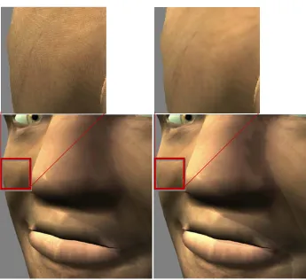
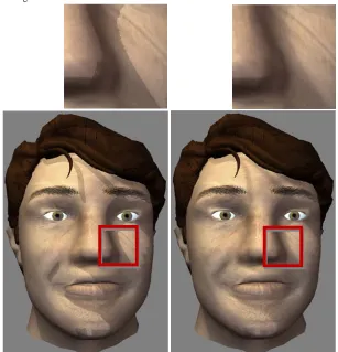
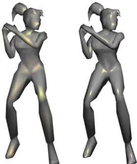
There are OpenGL extension to have per fragment lighting or one can write a shader program incorporating the same equations but on fragment level. In figure 2.1 this is shown on a low polygon model. On the left you can clearly see how the specular highlight is flowing from one point (on the leg), in contrast to the model on the right. There even are highlights showing in places where a vertex based lighting model shows nothing at all (for example at the feet)

Going from a vertex based model to a fragment based model clearly gives visual improvements however at a greater computational cost. Since normally only the equation is done on each vertex and now for every fragment. To make it clearer, if the model consists of about a 1000 vertices then the vertex lighting model is executed a 1000 times, however for a fragment based lighting model this can easily add up to 1.310.720 executions every render cycle for a screen resolution of 1280x1024 with the same model.

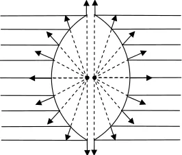
For the lighting calculation a couple of vectors are important, they are shown in figure 2.2.

•

•

•

•

These are all unit length vectors.

Figure 2.1: Left the model has vertex lighting and on the right per fragment lighting. A fragment shader is the same

as a pixel shader. Usually in OpenGL the term fragment is used and in DirectX pixel. On a monitor the term pixels is common, however before that in the renderpipline they are more fragments then pixels.

Figure 2.2: The basic vectors used in lighting equations. View, Reflection, Normal and Light vector.

V R N L

V

R

N

LIGHTING MODELS

Default OpenGL lighting

E m i s s i o n

The emission is simply an RGB color that can be assigned to the fragment or vertex. It isn't affected by any other attribute. This implies, for instance, that when emission if full white, the object being rendered will always be full white. As shown in the equation below.

The resulting color, the Emission component Material emission color

A m b i e n t

The material can be set to an ambient color; a light can be set to an ambient color and the world ambient an RGB value. The world ambient color is scaled by the material ambient color. And for each light the ambient color is scaled with material ambient color. Both of them are added up and form the ambient component.

With the diffuse attribute the normal vector comes into play. Based upon the normal it checks if the light is hitting vertex.

The light unit vector from the vertex to the light source. The diffuse component

The unit normal vector. The light diffuse color.

The material diffuse color.

The max function returns the greater value of two values. Thus here if the dot product between L and N is negative the function returns zero. If zero is the result the diffuse component is discarded, this causing one sided lighting.

This is also known as the Lambertian diffuse model, because it depends on Lambert's law; it gives ideal diffuse reflection (intensities) in any direction.

S p e c u l a r

The specular component like the diffuse component also depends on the normal vector, but also uses the reflection vector. The reflection vector is calculated using the Blinn method, where it is better known as the half-vector.

Normally the Phong specular reflection color is computed:

LIGHTING MODELS

Default OpenGL lighting

2

The reflection vector. The specular component

Material shininess, also referred to as the specular exponent. Light specular color (also referred as the intensity).

Material specular color (same remark as L_s).

Blinn proposed an optimized reflection calculation, by introducing the half-vector.

The half-vector. Sum of the Light and View vector.

A t t e n u a t i o n

If the current attribute calculations are put together, a light source would have an infinity range of effect. This is often used for static environment lighting (like having sun light). For lights that are limited by a range of effect the attenuation factor is used as a scalar and is based on three coefficients.

The attenuation factor. constant attenuation. linear attenuation.

quadratic attenuation.

The distance between the vertex/fragment and the light source.

Normal vectors in OpenGL can be defined per face or per vertex. If defining a normal per face then the normal is commonly defined as a vector which is perpendicular to the surface. In order to find a perpendicular vector to a face, two vectors coplanar with the face are needed. Afterwards the cross product will provide the normal vector, i.e. a perpendicular vector to the face.

B l i n n - p h o n g s h a d i n g c a l c u l a t i o n

The only thing that has been left out here is the "spotlight effect". The spot light effect defines a boundary (alike the attenuation factor) and is multiplied with the attenuation factor.

The spot effect factor.

The light spot direction (unit vector).

The light spot exponent to control the intensity distribution.

This completes the light model for the default OpenGL lighting; there are however additional settings and possibilities provided by OpenGL. Also there was no texturing involved (not to mention multi texturing), and no blending (transparency). A word on these issues is given in section 2.7 “Lighting and texturing” on page 18, since the other lighting models also have the same issues on these topics a word given on this is done afterwards.

LIGHTING MODELS

Cook-Torrance

. . .

2 . 2 C O O K - T O R R A N C E

The Cook-Torrance model[35] is a specular component lighting model, and is based on the model of Torrance and Sparrow. The model takes a Fresnel term to modify the reflected amount of light in different angles. By doing this it introduces microscopic facets on a surface, where every facet is a ideal reflector.

A base color, this can be the diffuse color or specular color. The distribution term for the facets orientations.

Which can be for example the Blinn function:

Roughness parameter 1 (a user selected scalar/constant). Roughness parameter 2 (the average gradient of the facets).

The half vector as shown in section “Default OpenGL lighting”. Can also be some other function for the reflection vector.

Other distribution function can be used (such as the Beckman distribution[5], is however more complex and performance intensive).

Describes the shadowing and masking effects between the micro facets.

The Fresnel reflection term corresponding to a material's index of refraction. The Fresnel term is here given for completeness.

The indice of refraction for a material (can be wavelength dependent or as stated by [5] "at least a color channel").

Because of the complexity often a simplification is used, created by C. Schlick[13]

Here and are the material's indices of refraction.

. . .

2 . 3 O R E N - N A Y A R

The model presented by Oren and Nayar[34] is a diffuse reflection model and differs from the Lambertion diffuse model as it introduces retro reflection (reflection back to the light source). The

LIGHTING MODELS

Environment mapping

2

equation presented here is based on the equations provided by [5], with some notation changes ( part of the equations provided in the book are only given in shader code).

The resulting diffuse component color.

The first part of the equation is the base diffuse color and resembles the Lambertian diffuse model.

The unit normal vector.

The unit light vector.

Light diffuse color.

Material diffuse color.

The sigma represents the roughness of the surface.

The angle between the light vector and the view vector.

The implementation of this model is quite instruction costly. In [5] they present a optimizing method by storing particular data in a texture and use the texture as a two dimensional lookup table and reduce the amount of instruction from 70 to 27 (for comparison: the Blinn-Phong model uses about 20 instructions).

. . .

2 . 4 E N V I R O N M E N T M A P P I N G

Originally developed by Blinn and Newell[14] environment mapping is a technique to reflect the surrounding on an object. It can however also be used as a replacement for global ambient or for specular highlighting. The downside is that some reflective object cannot “easily” reflect itself when using realtime generated environment maps. Note that self reflection is only possible on concave objects. By default the backface culling is enabled in OpenGL (this means that the back side of a polygon is not being rendered) and therefore it would be possible to render itself on itself with a very small near offset for the camera. In practice this only gives a lot of trouble with artifacts and incorrect reflections.

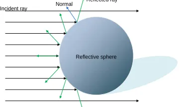
S p h e r e m a p p i n g

Basically this method creates, using for example the reflection vector, texture coordinates for a lookup texture. This texture can be seen as a textured sphere containing a complete panoramic environment obtained from an external source (for example a real world image) or a real-time

D = max N L{ ⋅ ,0}L_dM_d(A+Bsin( )α tan( )β max{cos(( )C,0)})

“

”

incident irradiance in any direction at a particular fixed point in space."

LIGHTING MODELS

Environment mapping

render with the off-screen view from the object towards the viewer. This is also known as Sphere mapping, and OpenGL supports this. Internally OpenGL uses the following formula to create the appropriate spherical st coordinates.

On a side node: "UV coordinates" is also often used instead of "ST coordinates" to denote texture coordinates, this is because they are often the same (U==S and V ==T). The st coordinates are Surface Texture Parameters and uv coordinates are Surface Parameters (for example used for NURBS).

and are the texture space coordinates. The reflection vector.

The unit view vector. The unit normal vector.

The reflection vector after normalization lies in the range of however for a texture it must

be in the range of therefore the scale by and the bias of .

In practice, any image loaded as a texture can be used for this method and the surprising part is that even when not "really" reflecting the actual surrounding, it often is sufficient realistic instead

Reflective sphere Incident ray Normal

Reflected ray

Figure 2.3: Spherical mapping where the reflection ray is used for lookup in a texture.

s Rx

LIGHTING MODELS

Environment mapping

2

of real-time environment mapping. Most important when using a non-realtime texture is to have the same coloring/tone as the environment.

Another method often used when looking at real-time environment-mapping is sharing of the environment map. Normally for every object that has some reflection it should have its own "per render cycle" updated environment map. However common practice is to use "one" environment map (created from a predefined point) for all reflective objects. These are performance related considerations, and real-time environments cannot afford to lose too much performance if the effect gain is minimal. Especially in video games this method is often used.

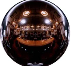
So we know now that environment mapping is a technique where we get the reflection from an image, and that this image can be a real photo (external source), or a real-time environment map. The most interesting part here is the real-time environment mapping. There are several techniques to create environment maps and to map them onto an object. The first one mentioned is spherical mapping. The dynamic creation for a spherical map is tricky, because one needs to render the reflective part with a possible optimal angle of 180 degrees (if not more for some mirror objects). To be precise, this is an off screen render pass, where the reflection view point is set to the origin of the object and the viewing direction is set to the inverted direction of the viewer (looking at the camera so to say). Then it captures (renders) the scene (without himself) into a texture (a texture buffer object bound to a logical color buffer bound to an FBO). However in perspective mode with a wide angle the resulting image gives a strong fisheye distortion. A solution to this is an orthographic mode, thus orthographic parallel rendering. To illustrate this, figure 2.6 simulates the effects of having a perspective camera (with a large angle, 180 degrees) in the middle of the object giving undesired 'pinch' effects in the resulting sphere map.

Figure 2.5: Example of static environment map (SGI).

LIGHTING MODELS

Environment mapping

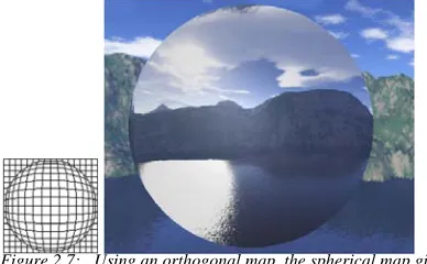
The image below shows a better effect of spherical mapping using an orthographic camera.

The main downside of spherical mapping is that it is view dependent, because the reflection map is created with the use of the inverted viewer direction. View independent methods are cube mapping and paraboloid mapping.

C u b e m a p p i n g

With cube mapping, all six directions are being rendered to textures, also called a cube map.

Each face is rendered by a different view direction with a 90 degrees angle (horizontal and vertical, in perspective mode), combining them to a cube map.

Retrieving the appropriate ST coordinates for mapping the reflection vector is sufficient.

The reflection vector is used from the center of the cube. A face is then selected based on the largest magnitude coordinate. The major axis, and in figure 2.9 this would be the "+X" face where

Figure 2.7: Using an orthogonal map, the spherical map gives better results.

“

”

cube.

Figure 2.8: A cube map, unfolded on the left and on the right the binding of its environment is illustrated. (http://www.developer.com/img/articles/2003/03/24/EnvMapTecIm01.gif)

LIGHTING MODELS

Environment mapping

2

the value x is >0 (otherwise it would hit the -X face) and x is in magnitude larger than the Y and Z values (x>Y , x>Z). To get the ST coordinates, the other two values are divided by the major axis (in the example: s=y/x,t=z/x) The new coordinates can then be used for the lookup in the texture[1].

This method creates realistic environment mapping however it uses significantly more resources since it has to render 6 times. If the environment map isn't updated every render cycle it is a good solution (or if graphics power doesn't matter).

P a r a b o l o i d m a p p i n g

The paraboloid mapping, created by W. Heidrich & H. Seidel [15] is similar to spherical mapping, however it uses two textures instead of one. Although this is known as a two pass rendering, it is possible to do it in one pass by using multi render targets (only if supported by the graphics hardware). The environment map is taken from the center of the reflective object and then the scene is divided into two hemispheres by rendering the front and the back or better said from the object perspective "rendering forward and backwards".

The encoding of the incoming rays reflected on the surface is given by:

The formula describes the paraboloid information using the image created by the camera (viewpoint) in an orthographic setup.

Notice that no reference to the z coordinate is used, this is because the viewing is along the z axis. In practice this means that the viewing point is set up in the middle of the object looking in some direction. A specific direction is not important since the calculations are in eye space (and therefore looking along the z axis), however usually the environment maps are aligned to the default coordinate system.

Figure 2.10: Paraboloid mapping, using only the front and back to map its environment.

f x y( , ) 1

2

--- 1

2

---(x2_+y2)

for x2_+y2_≤1 –

LIGHTING MODELS

Environment map as Ambient light

The texture lookup for the front face is given by

Where R is the reflection vector calculated using the normal and view vector ( ).

. . .

2 . 5 E N V I R O N M E N T M A P A S A M B I E N T L I G H T

Instead of only reflection the environment map can be used as a cheap method for having a better ambient lighting. The Ambient light part for example in the Blinn-phong model can be replaced with this approach. The idea is to take the colors from the environment and use them as a light source. The negative side on this approach is that bright colors have great impact, for there is no light intensity. For example a red ball gives the same light intensity as a red light. But this is acceptable for it gives the impression of a better light environment.

This is usually done in several steps

•

•

•

By down sampling the environment map it gives also a blur effect, because of the linear interpolation during the texture mapping (sampling down and then stretch it up).

. . .

2 . 6 S P H E R I C A L H A R M O N I C S

With spherical harmonics it is possible to approach accurate diffuse reflection based on its surrounding (light probe). R. Ramamoorthi and P. Hanrahan presented in 2001 a method to use spherical harmonics for the diffuse term based on a light probe[16] and in 2002 a paper was presented by J. Kautz, P. Sloan & J. Snyder for using spherical harmonics as a low-frequency lighting in a BRDF shading model[17].

T h e d e f i n i t i o n

Spherical harmonics are basis functions, which can be seen as signals that can be scaled and combined together to approximate an original function[18] over a 2 dimensional unit sphere.

LIGHTING MODELS

Spherical harmonics

2

The definition for Spherical harmonics ("real spherical harmonics function y") is:

The scaling factor to normalize the functions.

The polynomial, from the set of associated Legendre polynomials.

With two arguments l and m. l is the band index from the natural numbers. A slight difference

from the original Legendre polynomials is the range, defined: becomes the

definition: .

The Legendre polynomials are defined in a recursive manner:

And the scaling factor is given by:

In [5] and [18] the following simplification is used for the spherical harmonics:

This gives a single indexed form of the spherical harmonics and is used later on in the reconstruction/projection of the original function.

P r o j e c t i o n

The reconstruction of the original function is approximated with the nth order function:

Where the coefficient is calculated by integrating the product of the function , which is a

two dimensional function defined over the unit sphere, and the spherical function .

Using the simplification the capped function becomes:

To fully reconstruct the function replace in the band limited function with .

The orange book[3] provides a detailed way to implement spherical harmonics and also provides the precomputed coefficients based on the light probes available from Devebec[39] and a optimized formula that can be easily implemented in a vertex shader program. The formula presented is based on the use of 9 basis function. Given by R. Ramamoorthi and P. Hanrahan[16]

LIGHTING MODELS

Spherical harmonics

9 basis functions are enough to reproduce the accurate diffuse reflection term (average error less than 1%).

Are derived constants.

Are the spherical harmonics coefficients. The normal vector

For completeness, the coefficients for the "Old town square lighting" are provided here. All the light probes available at Devebec's website were also processed and the coefficients are also available in the orange book[3].

Diffuse =c₁l₂₂ N_x2 _N

y2

–

( ) c₃L₂₀N_z2 _c

4L00–c5L20 2c1(L2–2–xy+L21xz+L2–1yz)

2c₂(L₁₁x+L_1–1y+L₁₀z)

+ + +

+

c₁ = 0.429043

c₂ = 0.511664

c₃ = 0.743125

c₄ = 0.886227

c₅ = 0.247708

c₁, , , ,c₂ c₃ c₄ c₅ L

N N_x N_yN_z

L_{00 0.871297 0.875222 0.864470}

L_{1–1 0.175058 0.245335 0.312891}

L_{10 0.034675 0.036107 0.037362}

L_{11 –0.004629–0.029448 –0.048028}

L_{2–2 –0.120535–0.121160–0.117507}

L_{2–1 0.003242 0.003624 0.007511}

L_{20 –0.028667–0.024926 –0.020998}

L_{21 –0.077359–0.086325 –0.091591}

L_{22 –0.161784–0.191783 –0.219152}

=

=

=

=

=

=

=

=

LIGHTING MODELS

Lighting and texturing

2

In figure 2.11 some examples are shown using the spherical harmonics applied on the HMI face model. No other lighting is used or any texturing, just the diffuse term calculated from the spherical harmonics is directly used as the final color.

. . .

2 . 7 L I G H T I N G A N D T E X T U R I N G

Looking at all the BDRF's there is one thing left out, the surface texturing. With texturing we can simulate a surface appearance by mapping an image to it. As shown previously in figure A.4. Together with a BDRF and appropriate parameter settings (for example the material index) a more realistic surface should be the result. But where does the texture come into play?

First off what is meant by "texturing"? As stated before "simulate a surface" but based on what? Textures are external produced images or procedural generated images. Basically this can be anything as long it is some image loaded into memory and is assigned as being a texture, but there are a couple of well known types of textures. First those that are used for tiling and show a certain material or composition, for example wood, brick, grass, skin etc. These textures are made so, that when they are tiled they fit exactly together and no seams are shown. Well at least the good ones! These textures can be said as being mesh independent since they are used to fit per polygon. The other texture is more or less bound to a mesh. The mesh has a set of ST coordinates and uses the specific texture to get the appropriate color information; the texture is as it were "stretched" over multiple polygons.

Within a BDRF the texture is often used as a replacement or extension to the material diffuse color. This sounds logical, since the diffuse color is the base for coloring an object, but this is not a given fact. There is also a possibility of having multi-texturing, where multiple textures are layered on top of each other. These need to be blended by some function, and depending on the application some layers must be treated different in the BDRF. This still seems to be an open field and is left to the creator's creativity/ingenuity. OpenGL supports several blending methods for multi texturing (Replace, Modulate, Decal, Blend, Add).

Figure 2.11: Spherical harmonics based on the coefficients from the orange book[3].

1: Old town square

2: Grace cathedral

3: Galileo’s tomb

4: Campus sunset

5: St. Peter’s Basilica

1 2 3

LIGHTING MODELS

Conclusion

In the previous section a texture from the environment is used as a substitute for reflecting the environment, or as a source for the environment light ambient. Other specialized textures might contain other information, for example a specular map which contains values of intensity of specular highlight. Such maps can be thought of as “material” maps as they contain information about the objects material properties.

. . .

2 . 8 C O N C L U S I O N

LIGHTING MODELS

. . . .

. . . .

3

B

UMP

MAPPING

ump mapping is a way to add details to a surface without adding new vertices[20]. This usually is done on a per fragment basis where for each fragment the normal vector is altered by some function. There are several techniques to do bump mapping, however in this section the two most prominent methods are given. First normal mapping[21] and as an extension parallax mapping based on the article from T. Welsh presented in the book ShaderX3Parallax Mapping with Offset Limiting: A PerPixel Approximation of Uneven Surfaces[11][22].

. . .

3 . 1 T H E N O R M A L V E C T O R

First let's get a better view on this normal vector and how this is retrieved per fragment. This usually involves three steps: the normal vector for a plane (in this case a polygon), then the normal per vertex by averaging the normal vectors from the planes sharing the same vertex and finally the normal per fragment by interpolating the normal from vertex to vertex. However with bump mapping the normal is altered and this can be done by some function or/and a lookup texture containing normal vectors.

N o r m a l v e c t o r p e r p o l y g o n

The best way to calculate the normal vector is from the smallest polygon unit, a triangle. A triangle is defined by three vertices where we can extract two coplanar vectors from.

The normal vector for this plane is then easily retrieved by the cross product between the two vectors.

The only thing left to do is to normalize the normal vector .

N o r m a l v e c t o r p e r v e r t e x

The normal per polygon is comparable to the flat shading state in OpenGL and gives an object a faceted look. The reflection over the complete polygon is the same. So the next step is to provide

B

Figuur 3.1: Calculate two coplanar vectors.

BUMP MAPPING

Light the bumps using normal maps

3

each vertex with the appropriate normal vector by averaging the normal vector and create a smooth shading effect (OpenGL also has a state for smooth shading).

In figure 3.3 the normal vectors for the polygons are denoted by and the normal vector that

we want to calculate is .

And at last normalize again.

N o r m a l v e c t o r p e r f r a g m e n t

From the normal vector per vertex to per fragment is a linear interpolation. This is normally done by the rendering pipeline when going from the vextex processor to the fragment processor.

. . .

3 . 2 L I G H T T H E B U M P S U S I N G N O R M A L M A P S

We can actually create bumps at vertex level (using the vertex normals), thereby creating certain effects. As they are usually averaged for "smooth shading" a hard edge for example can be created. But let's get to an actual bump mapping technique called normal mapping. A normal map is a texture, an internal frame buffer or some other buffer, but usually a texture is meant, that contains the new normal vectors. In the previous sections where the normal calculation was explained, the normal resided in object space. During normal rendering the normal is moved into eye space in the vertex processor (the normal is given per vertex) and is automatically interpolated within the fragment processor. There the lighting calculation can be done on a per fragment basis (still in eye space). Now the normal comes from a texture and also resides in a certain space. The first possible space is the object space, and another possible option is a local surface space also called tangent space.

N o r m a l m a p s a n d o b j e c t s p a c e

The normal vectors are stored in object space, thus they are pointing in their actual directions and are mesh dependent. Whenever an object translates/rotates (moving into world/eye space) the normal vectors or the view and light vector must be moved into the same space. Thus every

Figuur 3.3: Per vertex normal averaging.

Vertex normal Polygon normal

N_v

N_p1 N_p2

N_p3 N_p4

N_p N_v

N_v Np1+Np2+Np3+Np4

4

---=

N_v

BUMP MAPPING

Light the bumps using normal maps

normal vector needs to be moved into eye space, or the view and light vector must be moved in the object space of the object.

The creation of normal maps in object space is usually done in the 3d editor (modeler) , using a high polygon model as reference. The normal vectors that are being stored are actually the vertex normal vectors from the high polygon model. Then the model is reduced to a lower polygon count and the normal map can be applied.

In the fragment shader the given texture coordinates (provided with each vertex) are used for lookup. The retrieved normal vector is then multiplied with the Modelview Matrix (the matrix containing the eye space information). However the modelview matrix is not used, but a special matrix called Normalmatrix. This is done because when the modelview matrix has some non-uniform scaling applied to it, it can deliver a wrong normal resulting in a normal that is not perpendicular to a surface.

In the image above on the left is the correct normal and tangent given, on the right the incorrect normal due to a non-uniform modelview matrix. To correct this, the normal is multiplied with the

transposed inverse modelview matrix [[3]. Note that when there are no special operations

on the modelview other then translation and rotation the default modelview matrix can be used (the 3x3 upper left sub matrix needs to be orthogonal).

N o r m a l m a p s a n d t a n g e n t s p a c e

The normal vectors are placed in a surface local space called tangent space. In this space it

assumes that every point is at the center (the origin) and that the unperturbed surface

normal at each point is . The view and light vectors must be converted into tangent space

using some matrix; this introduces the tangent and bitangent component for each vertex. The combination of the normal, tangent and bitangent vectors is called the tangent space matrix which is a 3x3 matrix containing the rotation and scaling for the tangent space per vertex. First to calculate the tangent and bitangent for a polygon.

T

N

T’ N’

Figuur 3.5: Left the correct Tangent and Normal vector, and on the right a skewed Normal due to non-uniform scaling.

M–1 ( )T

0 0 0 0 0 1

ܸ_ଵ ܸଷ

ܸ_ଶ

N _B

T

BUMP MAPPING

Light the bumps using normal maps

3

Denote the vertices representing their space position .

The edge vectors .

Represent the texture coordinates for the vertices .

The texture coordinates for the edges .

The tangent vector .

The bitangent vector .

The next step is to average and normalize the tangent and bitangent vectors for each vertex the same way as done with the normal vector. Eventually add the Gram-Schmidt orthogonalization to make the normal, tangent, bitangent vectors orthogonal. Note that the bitangent can also be calculated by taking the cross product of the normal and tangent vector.

The main advantage of tangent space textures is that it is mesh independent, it can be reused. For example can it be used for symmetrical parts of a model (by simple reversing the axis of symmetry) and another usage could be tiled textures for example detail maps (a multi textured normal map, one for distance and one for close up).

Let's see what this in practice means. In figure 3.7 a sphere is used and some unwrapping method is applied to define the st coordinates; this is shown below in the left image in figure 3.7. Then for every pixel in the destined texture the normal vector is saved in color space (this space ranges from 0.0 to 1.0, where the normal usually is from -1.0 to 1.0, thus a small conversion is needed). Saving the normal vectors in object space is shown in the middle figure and in tangent space shown in the right figure. In object space the color varies strongly and in tangent space the color is constant, this directly shows why the tangent space map is useable for multiple objects. Although the object is a sphere the normal in the tangent map stays constant and delivers the same effect.

E₁ V₂ V₁

BUMP MAPPING

Creating a normal map

This makes it easier to work with and to create them. A good programming strategy would be to have the source textures in tangent space and once in the program create object space maps from the tangent space maps; this can reduce the amount of operations. Object space maps are however not practical with dynamic models (animated) and for using the tangent space map the tangent matrix needs to be recalculated (with dynamic models the normal is usually recalculated, and in this case the tangent and bitangent vectors must also be recalculated). Mutation to the tangent map 'can' be done by hand which would be almost impossible in object space.

. . .

3 . 3 C R E A T I N G A N O R M A L M A P

Here a possible solution is given on how to make dynamic normal maps in Tangent space. The approach is based on the shader available from RenderMonkey[40]. For each fragment the 8 direct surrounding fragments are taken then the slopes for x and y are calculated using the Sobel filter and a normal vector is retrieved. The input can be a diffuse map or a heightmap, as the color difference between the selected fragments is used to determine the slope. Note that this method can result in “undesired” bumps (example incorrect direction) as the filter kernel determines how the slope is calculated. It is not a defintive way on how to calculate dynamic “correct” normals, but it delivers acceptable normals. Here the algorithm is presented:

The normal vector (still needs to be normalized before storing). A control vector for adjusting the intensity of the bump and direction.

A surrounding fragment color .

The temporary variables are the components.

For creating the normal map using this filter or a similar filter the best source is a heigh map. A height map image contains as the name implies the height at each pixel. Usually this is saved in one channel and can be seen as a grey colored image (notice that the given filter above uses all the color channels). This actually means that creating a bump map is rather easy. By drawing a grey map, which can be done in the actual render program (for dynamic bumps) or "off-line" using a

Table 3.1: Surrounding fragments used for filtering.

BUMP MAPPING

Parallax mapping

3

drawing program (like Gimp). An example is shown in figure 3.8. Using a simple brushed text, convert the image and use it (figure 3.9).

. . .

3 . 4 P A R A L L A X M A P P I N G

This technique is more and more used in today's 3D real-time programs (mainly games). The main advantage of parallax mapping is the ability of occlusion which is not possible with the normal mapping technique explained in the previous section, hence it is also known as 'virtual displacement mapping' or 'offset mapping'. Where the 'displacement mapping' technique actually moves vertices this technique does not, it actually moves st coordinates instead. The normal map here is optionally, as the normal can be calculated on the fly. The main input for this technique is a depth map (or height map depending on its usage). The depth map is a texture where each pixel is a depth value, this only uses one channel and is often placed in the alpha channel (the RGB channels can then be used for the normal, diffuse color or other information). Parallax mapping can be implemented in several ways, for giving a good view on this techniques it is explained here following the implementation by T. Welsh [22].

In figure 3.10 the problem is illustrated. The surface is rough and a polygon is plain flat and the texture used on the polygon is also flat (by default the st coordinates are linearly interpolated from vertex to vertex). If we look at the polygon we would get the st texture coordinates at point A, however due to the roughness is should be st texture coordinate B.

Figuur 3.8: Left the height map and on the right the normal map based on the height map.

Figuur 3.9: Left the rendering without bump mapping, and on the right with bump mapping.

ܣ௦௧

ܤ௦௧

Surface

Polygon

BUMP MAPPING

Parallax mapping

To approximate the correct st texture coordinate an offset is calculated using the eye vector and the surface represented by a depth map.

To compute the offset three components are needed. The starting texture coordinate, that is, the interpolated coordinate that would be used by default for mapping a texture to the polygon. The surface height is needed. Here the starting texture coordinate can be used for looking this up in the depth map. And third the normalized eye vector in tangent space, this involves the tangent space where for each vertex the tangent matrix must be supplied (the calculation is the same as shown in the previous section "normal maps and tangent space"). The values in the depth map range from 0.0 to 1.0. To adjust the height a scalar and a bias are used for calibration,

, where is the height retrieved from the depth map. The formula

to get an approximated new texture coordinate:

V is the View vector in tangent space. (In the vertex processor moved into tangent space, and in the fragment processor normalized.)

As can be seen in figure 3.11 the approximated coordinate is flawed, especially for a steep rough surface. This can actually end in an unrecognizable surface; the paper by T. Welsh[22] suggests

a simplified "offset limiting" . Using this formula the offset can never

be larger than the maximum height.

The normal is in no way altered or whatsoever using this technique, the only thing that has been done is moving the st coordinate to simulate occlusion. This is done in addition to bump mapping, so the actual normal perturbations are still to be done by some method. This can be the normal mapping technique, or calculate the normal on the fly using the depth map information.

ܣ௦௧

ܤ௦௧

Depthmap/heightmap

Polygon

Offset

Figuur 3.11: An approach to simulate this roughness.

height = H_stScale+Bias H_st

B_st A_st height*Vxy

V_z

---⎝ ⎠

⎛ ⎞

+ =

BUMP MAPPING

. . . .

. . . .

4

R

EAL

-

TIME

SHADOW

CASTING

hadow can give visual cues to the position of an object in an environment and adds a great deal of realism. In this particular case for rendering a face, self-shadowing is important. The shadow from the hair, nose and eye socket give more information on how the face is lit. There are several shadow casting techniques possible to implement and each has its strong and weak points[23][24]. Instead of explaining all kinds of shadow techniques only the one used in this project will be discussed, which is shadow mapping. Previous work on shadow mapping within the HMI department has also been done by B. Kevelham[25] in a project for obtaining his Master degree (the project was carried out at MIRALab). A small summary on advantages of shadow mapping are:

•

•

•

•

A shadow is created by an object blocking the light rays, this is shown in figure 4.1.

Everything in the shadow volume receives no light from the light source because of the occluder. The occluder and the shadow receiver are usually part of the geometry used in the scene. Note the mention of "usually" in the previous sentence; because we are dealing with virtual generated scenes it does not necessarily have to be the geometry that creates the shadow (for example a predefined shadow map texture can be used).

. . .

4 . 1 S H A D O W M A P P I N G

Shadow mapping is a 2-pass rendering method. This means that at least two sequential render passes are necessary to create/visualize shadows. The first one is the shadow pass, where a depth buffer is used to store the depth values from the lights 'viewpoint'. The shadow pass is also mentioned as being the light pass, however although the shadow pass is using light-entity information (translation and rotation) it does not have to do anything with the lighting algorithm itself. The lighting itself can also be a different pass; this is also shown in the next section on Deferred shading.

The second pass is the normal rendering pass and the depth buffer from the shadow pass is used to check whether a fragment falls in the shadow or not by comparing the depth from the current viewpoint with the depth from the light's viewpoint.

For the first pass to work we need to render off-screen. This can be done by using the framebuffer object extension. The framebuffer buffer object is set up to only contain de the depth values, thus

S

Occluder

Shadowreceiver Shadowvolume

Lightsource

Figure 4.1: Simplified illustration of casting shadows.

REAL-TIME SHADOW CASTING

Shadow mapping

4

a depth buffer is added to the framebuffer. There is no need for any color buffer as it is not needed for the actual render pass. The framebuffer object now easily provides access to the depth buffer by using a texture binding with the logical depth buffer and passing it by a uniform sampler variable in the shader program. The render pass is done as follows:

STEP 1

In the modelview mode (thus using the modelview matrix stack) set the camera/viewpoint to the light source position and rotation. Depending on the light source type the amount of passes to render might differ. A light point can cast shadows in all directions; usually this is solved by rendering 6 times to create a depth environment map stored in a cube map. Note that it also is an option to use the paraboloid technique instead of a cubemap.

For a spot light a single render pass is sufficient, using the rotation from the spot light to setup the viewpoint. And for the directional light type an orthographic projection is used (note that the translation of the light’s viewpoint is depended on the view of the 'user' and should cover every region the 'user' also can see)

STEP 2

REAL-TIME SHADOW CASTING

Shadow mapping

The depth buffer needs to be setup for comparison, in practice this can be done in two ways.

•

•

With the hardware support we don't really have to worry about this, thus the normal solution is to use a depth buffer attached to the FBO. However if for some reason it is needed to write the values our self, the depth can be written in the RGB channels by converting the depth value into a value that can be stored in the channels. This is shown in the equation below.

The depth value for a given fragment. Which is usually the z value in view space. The color bit depth, which is normally 8bit per channel, the value here is then 256.

The resulting color vector

By reversing this process the depth is retrieved again.

For the hardware support the depth is automatically written in the buffer and also follows the depth test function. In figure 4.3 a sample is given of what a depth buffer looks like when it is

Figure 4.2: On the left there is Z-fighting and on the right a polygon offset is given.

D′ Db

C_r floor D( )′ D″ b D( ′–C_r) C_g floor D( ″)

= = = =

C_r C_r1

b

---C_g C_g1

b

---=

=

D b

REAL-TIME SHADOW CASTING

Soft shadows using shadow mapping

4

used as a texture. The figure on the left gives the normal "colored" result of the rendering, the middle figure the original depth texture and on the right the contrast has been slightly enhanced to make it more visible.

Note that when using the depth buffer, that has been set up for comparison (which is needed for shadow checking), as a texture the result is always blank. The image from figure 4.3 shown as the depth buffer has not been set up for depth comparison. This has been tested on an NVidia (6800gt) and ATI (x700) card and both only show the depth when they are not in comparison mode.

Now we have the depth written in the buffer, the next thing we need is the shadow matrix so that we can move a vertex into the shadow space. To get the appropriate depth value from the depth buffer, the texture coordinates must be calculated for the depth which corresponds to the current fragment.

is the vertex in world space (the space between object and view space).

The shadow map is then accessed using . The value that is retrieved from the shadow map

is then compared with the current de