Face Recognition via Robust Auxiliary Dictionary Learning

(1)

Face Recognition via Robust Auxiliary Dictionary Learning

P.VEENA D.RAJA SEKHAR

Student Assistant Professor

Department of ECE (DECS) Department of ECE (DECS)

G.Pullaiah College Of Engineering & Technology G.Pullaiah College Of Engineering & Technology Kurnool, Andhra Pradesh, India Kurnool, Andhra Pradesh, India

Email.Id: [email protected] Guide Email id: [email protected]

ABSTRACT

This paper mainly addresses the building of face recognition system by using Principal Component Analysis (PCA). PCA is a statistical approach used for reducing the number of variables in face recognition. In PCA, every image in the training set is represented as a linear combination of weighted eigenvectors called eigenfaces. These eigenvectors are obtained from covariance matrix of a training image set. The weights are found out after selecting a set of most relevant Eigenfaces. Recognition is performed by projecting a test image onto the subspace spanned by the eigenfaces and then classification is done by measuring minimum Euclidean distance. A number of experiments were done to evaluate the performance of the face recognition system. In this thesis, we used a training database of students of Electronics and Telecommunication Engineering department, Batch-2007, Rajshahi University of Engineering and Technology, Bangladesh.

I. INTRODUCTION

Over the last ten years or so, face recognition has become a popular area of research in computer vision and one of the most successful

applications of image analysis and

understanding. Because of the nature of the

problem, not only computer science

researchers are interested in it, but

neuroscientists and psychologists also. It is the general opinion that advances in computer vision research will provide useful insights to neuroscientists and psychologists into how human brain works, and vice versa [1].The goal is to implement the system (model) for a particular face and distinguish it from a large number of stored faces with some real-time variations as well. It gives us efficient way to find the lower dimensional space. Further this algorithm can be extended to recognize the gender of a person or to interpret the facial expression of a person. Recognition could be carried out under widely varying conditions like frontal view, a 45° view, scaled frontal view, subjects with spectacles etc are tried, while the training data set covers limited views. The algorithm models the real-time varying lighting conditions as well. But this is

out of scope of the current implementation. The aim of this research paper is to study and develop an efficient MATLAB program for face recognition using principal component analysis and to perform test for program optimization and accuracy. This approach is preferred due to its simplicity, speed and learning capability [2].

FACE RECOGNITION

Face recognition is a biometric which uses computer software to determine the identity of the individual. Face recognition falls into the category of biometrics which is ―the automatic recognition of a person using distinguishing traits‖ [6]. Other types of biometrics include fingerprinting, retina scans, and iris scan.

Eigenface-based Recognition

2D face recognition using eigenfaces is one of the oldest types of face recognition.

Turk and Pentland published the

groundbreaking ―Face Recognition Using Eigenfaces‖ in 1991. The method works by

analyzing face images and computing

(2)

eigenvectors. The comparison of eigenfaces is used to identify the presence of a face and its identity.

There is a five step process involved with the system developed by Turk and Pentland. First, the system needs to be initialized by feeding it a set of training images of faces. This is used these to define the face space which is set of images that are face like. Next, when a face is encountered it calculates an eigenface for it. By comparing it with known faces and using some statistical analysis it can be determined whether the image presented is a face at all. Then, if an image is determined to be a face the system will determine whether it knows the identity of it or not. The optional final step is that if an unknown face is seen repeatedly, the system can learn to recognize it.

The eigenface technique is simple, efficient, and yields generally good results in controlled circumstances [1]. The system was even tested to track faces on film. There are also some limitations of eigenfaces. There is limited robustness to changes in lighting, angle, and distance [6]. 2D recognition systems do not capture the actual size of the face, which is a fundamental problem [4]. These limits affect the technique‘s application with security cameras because frontal shots and consistent lighting cannot be relied upon.

3D Face Recognition

3D face recognition is expected to be robust to the types of issues that plague 2D systems [4]. 3D systems generate 3D models of faces and compare them. These systems are more accurate because they capture the actual shape of faces. Skin texture analysis can be used in conjunction with face recognition to improve accuracy by 20 to 25 percent [3]. The acquisition of 3D data is one of the main problems for 3D systems.

How Humans Perform Face Recognition

It is important for researchers to know the results of studies on human face recognition [8]. Knowing these results may help them develop ground breaking new methods. After

all, rivaling and surpassing the ability of humans is the key goal of computer face recognition research. The key results of a 2006 paper ―Face Recognition by Humans: Nineteen Results All Computer Vision Researchers Should Know About‖ are as follows:

1. Humans can recognize familiar faces in very low-resolution images.

2. The ability to tolerate degradations

increases with familiarity.

3. High-frequency information by itself is

insufficient for good face recognition

performance.

4. Facial features are processed holistically.

5. Of the different facial features, eyebrows are among the most important for recognition.

6. The important configural relationships appear to be independent across the width and height dimensions.

7. Face-shape appears to be encoded in a slightly caricatured manner.

8. Prolonged face viewing can lead to high level aftereffects, which suggest prototype-based encoding.

Staring at the faces in the green circles will cause one to misidentify the central face with the faces circled in red. This is an example of face aftereffects [8].

9. Pigmentation cues are at least as

important as shape cues.

(3)

11. Contrast polarity inversion dramatically impairs recognition performance, possibly due to compromised ability to use pigmentation cues.

Photograph during the recording of ―We Are the World.‖ This figure demonstrates how polarity inversion effects face recognition in humans. Several famous artists are in the picture including Ray Charles, Lionel Ritchie, Stevie Wonder, Michael Jackson, Tina Turner, Bruce Springstein, and Billy Joel though they are very difficult to identify.

12. Illumination changes influence

generalization.

13. View-generalization appears to be

mediated by temporal association.

14. Motion of faces appears to facilitate subsequent recognition.

15. The visual system starts with a

rudimentary preference for face-like patterns.

16. The visual system progresses from a piecemeal to a holistic strategy over the first several years of life.

17. The human visual system appears to

devote specialized neural resources for face perception.

18. Latency of responses to faces in

inferotemporal (IT) cortex is about 120 ms, suggesting a largely feed forward computation.

19. Facial identity and expression might be processed by separate systems.

FACE RECOGNITION PROCESS

One of the simplest and most effective PCA approaches used in face recognition systems is the so-called eigenface approach. This approach transforms faces into a small set of essential characteristics, eigenfaces, which are

the main components of the initial set of learning images (training set). Recognition is done by projecting a new image in the eigenface subspace, after which the person is classified by comparing its position in eigenface space with the position of known individuals [3]. The advantage of this approach over other face recognition systems is in its simplicity, speed and insensitivity to small or gradual changes on the face. The problem is limited to files that can be used to recognize the face. Namely, the images must be vertical frontal views of human faces. The whole recognition process involves two steps:

A. Initialization process

B. Recognition process

The Initialization process involves the following operations:

i. Acquire the initial set of face images called as training set.

ii. Calculate the Eigenfaces from the training set, keeping only the highest eigenvalues. These M images define the face space. As new faces are experienced, the eigenfaces can be updated or recalculated.

iii. Calculate distribution in this

M-dimensional space for each known person by projecting his or her face images onto this face-space.

These operations can be performed from time to time whenever there is a free excess operational capacity. This data can be cached which can be used in the further steps eliminating the overhead of re-initializing, decreasing execution time thereby increasing the performance of the entire system [4].

Having initialized the system, the next process involves the steps:

i. Calculate a set of weights based on the input image and the M eigenfaces by projecting

the input image onto each of the

(4)

ii. Determine if the image is a face at all (known or unknown) by checking to see if the image is sufficiently close to a ―free space‖.

iii. If it is a face, then classify the weight pattern as either a known person or as unknown.

iv. Update the eigenfaces or weights as either a known or unknown, if the same unknown person face is seen several times then calculate the characteristic weight pattern and

incorporate into known faces. The

last step is not usually a requirement of every system and hence the steps are left optional and can be implemented as when the there is a requirement.

III. EIGENFACE ALGORITHM

Let a face image Γ(x, y) be a two dimensional M by N array of intensity values. In this thesis, I used a set of image by 200 × 149 pixels. An image may also be considered as a vector of dimension M × N, so that a typical image of size 200 × 149 becomes a vector of dimension 29,800 or equivalently a point in a 29,800 dimensional space.

Fig-1:Conversion of M × N image into MN ×1 vector

Step1: prepare the training faces

Obtain face images I1, I2, I3, I4 , . . . IM (training faces). The face images must be centered and of the same size.

Step 2: Prepare the data set

Each face image Ii in the database is transformed into a vector and placed into a training set S.

In My example M = 34. Each image is transformed into a vector of size MN × 1 and placed into the set. For simplicity, the face images are assumed to be of size N × N resulting in a point in dimensional space. An ensemble of images, then, maps to a collection of points in this huge space.

Step 3: compute the average face vector

The average face vector (Ψ) has to be calculated by using the following formula:

Step 4: Subtract the average face vector

The average face vector Ψ is subtracted from the original faces and the result stored in the

variable ,

Step 5: Calculate the covariance matrix

We obtain the covariance matrix C in the following manner,

Step 6: Calculate the eigenvectors and eigenvalues of the covariance matrix

The covariance matrix C in step 5 has a

dimensionality of , so one would have

(5)

eigenfaces. Computationally, this is not very efficient as most of those eigenfaces are not useful for our task. In general, PCA is used to describe a large dimensional space with a relative small set of vectors [3].

Compute the

eigenvectors _of

AAT

The matrix AAT is very large - -  not practical!!!

Step 6.1: consider the matrix

Step 6.2: compute eigenvectors vi of L= AT A

What is the relationship between ui and vi ?

where, Thus, C = AAT and L

= ATA have the same eigenvalues and their

eigenvectors are related as follows:

Note 1: C = AAT can have upto N2 eigenvalues and eigenvectors.

Note 2: L = ATA can have upto M eigenvalues and eigenvectors.

Note 3: The M eigenvalues of C = AAT (along

with their corresponding eigenvectors)

correspond to the M largest eigenvalues of L =

ATA (along with their corresponding

eigenvectors).

Where vi is an eigenvector of L = ATA From this simple proof we can see that A vi is an eigenvector of C = AAT. The M eigenvectors

of L = ATA are used to find the M eigenvectors ui of C that form our eigenface basis:

Where, ui are the Eigenvectors i.e. Eigenfaces.

Step 7: keep only K eigenvectors

(corresponding to the K largest eigenvalues)

Eigenfaces with low eigenvalues can be omitted, as they explain only a small part of Characteristic features of the faces.

P R I N C I P A L C O M P O N E N T A N A L Y S I S

In principal components analysis (PCA) and factor analysis (FA) one wishes to extract from a set of p variables a reduced set of m components or factors that accounts for most of the variance in the p variables. In other words, we wish to reduce a set of p variables to a set of m underlying superordinate dimensions.

These underlying factors are inferred from the correlations among the p variables. Each factor is estimated as a weighted sum of the p variables. The ith factor is thus

p ip i

i

i W X W X W X

F  ₁ ₁ ₂ ₂

One may also express each of the p variables as a linear combination of the m factors,

j m mj j

j

j A F A F A F U

X  1 1 2 2 

where Uj is the variance that is unique to

variable j, variance that cannot be explained by any of the common factors.

Goals of PCA and FA

One may do a PCA or FA simply

to reduce a set of p variables to m

(6)

physiological response to four hours of cold-restraint. They first subjected the 19 predictor variables to a FA. They extracted five factors, which were labeled Exploration, General

Activity, Metabolic Rate, Behavioral

Reactivity, and Autonomic Reactivity. They then computed for each subject scores on each of the five factors. That is, each subject‘s set of scores on 19 variables was reduced to a set of scores on 5 factors. These five factors were then used as predictors (of the single criterion) in a stepwise multiple regression.

One may use FA to discover and

summarize the pattern of intercorrelations among variables. This is often called

Exploratory FA. One simply wishes to group together (into factors) variables that are highly correlated with one another, presumably because they all are influenced by the same underlying dimension (factor). One may also then operationalize (invent a way to measure) the underlying dimension by a linear combination of the variables that contributed most heavily to the factor.

If one has a theory regarding what basic dimensions underlie an observed event, e may engage in Confirmatory Factor Analysis. For example, if I believe that performance on standardized tests of academic aptitude represents the joint operation of several basically independent faculties, such as Thurstone‘s Verbal Comprehension, Word Fluency, Simple Arithmetic, Spatial Ability, Associative Memory, Perceptual Speed, and General Reasoning, rather than one global intelligence factor, then I may use FA as a tool to analyze test results to see whether or not the various items on the test do fall into distinct factors that seem to represent those specific faculties.

Psychometricians often employ FA in test construction. If you wish to develop a test that measures several different dimensions, each important for some reason, you first devise questions (variables) which you think will measure these dimensions. For example, you may wish to develop a test to predict how well an individual will do as a school teacher. You decide that the important dimensions are

Love of Children, Love of Knowledge, Tolerance to Fiscal Poverty, Acting Ability, and Cognitive Flexibility. For each of these dimensions you write several items intended to measure the dimension. You administer the test to many people and FA the results. Hopefully many items cluster into factors representing the dimensions you intended to measure. Those items that do not so cluster are rewritten or discarded and new items are written. The new test is administered and the results factor analyzed, etc. etc. until you are pleased with the instrument. Then you go out and collect data testing which (if any) of the factors is indeed related to actual teaching performance (if you can find a valid measure thereof) or some other criterion (such as teacher‘s morale).

There are numerous other uses of FA that you may run across in the literature. For example, some researchers may investigate the differences in factor structure between groups. For example, is the factor structure of an

instrument that measures

socio-politico-economic dimensions the same for citizens of the U.S.A. as it is for citizens of Mainland China? Note such various applications of FA when you encounter them.

A Simple, Contrived Example

Suppose I am interested in what influences a consumer‘s choice behavior when e is shopping for beer. I ask each of 20 subjects to rate on a scale of 0-100 how important e considers each of these qualities when deciding whether or not to buy the six pack: low COST of the six pack, high SIZE of the bottle (volume), high percentage of ALCOHOL in the beer, the REPUTATion of the brand, the COLOR of the beer, nice AROMA of the beer, and good TASTE of the beer. Here are the contrived data, within a short SAS program that does a PCA on them:

DATA BEER;

INPUT COST SIZE ALCOHOL REPUTAT COLOR AROMA TASTE;

CARDS;

--- see the data in the file

(7)

PROC FACTOR;

Checking For Unique Variables

Aside from the raw data matrix, the first matrix you are likely to encounter in a FA is the correlation matrix. Here is the correlation matrix for our data:

COST SIZE ALCOHOLREPUTATCOLOR AROMA TASTE

COST 1.00 .83 .77 -.41 .02 -.05 -.06

SIZE .83 1.00 .90 -.39 .18 .10 .03

ALCOHOL .77 .90 1.00 -.46 .07 .04 .01

REPUTAT -.41 -.39 -.46 1.00 -.37 -.44 -.44

COLOR .02 .18 .07 -.37 1.00 .91 .90

AROMA -.05 .10 .04 -.44 .91 1.00 .87

TASTE -.06 .03 .01 -.44 .90 .87 1.00

Unless it is just too large to grasp, you should give the correlation matrix a good look. You are planning to use PCA to capture the essence of the correlations in this matrix. Notice that there are many medium to large correlations in this matrix, and that every variable, except reputation, has some large correlations, and reputation is moderately correlated with everything else (negatively). There is a statistic, Bartlett‘s test of sphericity, that can be used to test the null hypothesis that our sample was randomly drawn from a population in which the correlation matrix was an identity matrix, a matrix full of zeros, except, of course, for ones on the main diagonal. I think a good ole Eyeball Test is generally more advisable, unless you just don‘t want to do the PCA, someone else is trying to get you to, and you need some ―official‖ sounding ―justification‖ not to do it.

If there are any variables that are not correlated with the other variables, you might as well delete them prior to the PCA. If you are using PCA to reduce the set of variables to a smaller set of components to be used in

additional analyses, you can always

reintroduce the unique (not correlated with other variables) variables at that time. Alternatively, you may wish to collect more data, adding variables that you think will indeed correlate with the now unique variable, and then run the PCA on the new data set.

One may also wish to inspect the Squared Multiple Correlation coefficient (SMC or R2 ) of each variable with all other variables. Variables with small R2 s are unique variables, not well correlated with a linear combination of the other variables.

Partial correlation coefficients may also be used to identify unique variables. Recall that the partial correlation coefficient between variables Xi and Xj is the correlation between two residuals,



Xi Xˆi.12..(i)..(j)..p



and



Xj Xˆj.12..(i)..(j)..p



A large partial correlation indicates that the variables involved share variance that is not shared by the other variables in the data set. Kaiser‘s Measure of Sampling Adequacy (MSA) for a variable Xi is the ratio of the sum of the squared simple r‘s between Xi and each other X to (that same sum plus the sum of the squared partial r‘s between Xi and each other X). Recall that squared r‘s can be thought of as variances.

 

 ₂ ₂

2

ij ij

ij

pr r

r MSA

(8)

marvelous, above .8 as meritorious, above .7 as middling, above .6 as mediocre, above .5 as miserable, and below .5 as unacceptable.

The MSA option in SAS‘ PROC FACTOR [Enter PROC FACTOR MSA;] gives you a matrix of the partial correlations, the MSA for

each variable, and an overall MSA computed across all variables. Variables with small MSAs should be deleted prior to FA or the data set supplemented with additional relevant variables which one hopes will be correlated with the offending variables.

For our sample data the partial correlation matrix looks like this:

COST SIZE ALCOHOL REPUTAT COLOR AROMA TASTE

COST 1.00 .54 -.11 -.26 -.10 -.14 .11

SIZE .54 1.00 .81 .11 .50 .06 -.44

ALCOHOL -.11 .81 1.00 -.23 -.38 .06 .31

REPUTAT -.26 .11 -.23 1.00 .23 -.29 -.26

COLOR -.10 .50 -.38 .23 1.00 .57 .69

AROMA -.14 .06 .06 -.29 .57 1.00 .09

TASTE .11 -.44 .31 -.26 .69 .09 1.00

MSA .78 .55 .63 .76 .59 .80 .68

O VERALL MSA = .67

These MSA‘s may not be marvelous, but they aren‘t low enough to make me drop any variables (especially since I have only seven variables, already an unrealistically low number).

Extracting Principal Components

We are now ready to extract principal components. We shall let the computer do most of the work, which is considerable. From p variables we can extract p components. This will involve solving p equations with p unknowns. The variance in the correlation matrix is ―repackaged‖ into p eigenvalues. This is accomplished by finding a matrix V of eigenvectors. When the correlation matrix R is premultiplied by the transpose of V and postmultiplied by V, the resulting matrix L

contains eigenvalues in its main diagonal. Each eigenvalue represents the amount of variance that has been captured by one component.

Each component is a linear combination of the p variables. The first component accounts for the largest possible amount of variance. The second component, formed from the variance remaining after that associated with the first component has been extracted, accounts for the second largest amount of variance, etc. The principal components are extracted with the restriction that they are orthogonal. Geometrically they may be viewed as dimensions in p-dimensional space where each dimension is perpendicular to each other dimension.

Each of the p variable‘s variance is standardized to one. Each factor‘s eigenvalue may be compared to 1 to see how much more (or less) variance it represents than does a single variable. With p variables there is p x 1 = p variance to distribute. The principal

components extraction will produce p

(9)

For our beer data, here are the eigenvalues and proportions of variance for the seven components:

COMPONENT 1 2 3 4 5 6 7

EIGENVALUE 3.31 2.62 .57 .24 .13 .09 .04

PROPORTION .47 .37 .08 .03 .02 .01 .01

CUMULATIVE .47 .85 .93 .96 .98 .99 1.00

Deciding How Many Components to Retain

So far, all we have done is to repackage the variance from p correlated variables into p uncorrelated components. We probably want to have fewer than p components. If our p variables do share considerable variance, several of the p components should have large eigenvalues and many should have small eigenvalues. One needs to decide how many components to retain. One handy rule of thumb is to retain only components with eigenvalues of one or more. That is, drop any component that accounts for less variance than does a single variable. Another device for deciding on the number of components to retain is the scree test. This is a plot with eigenvalues on the ordinate and component number on the abscissa. Scree is the rubble at the base of a sloping cliff. In a scree plot, scree is those components that are at the bottom of the sloping plot of eigenvalues versus component number. The plot provides a visual aid for deciding at what point including additional components no longer increases the amount of variance accounted for by a nontrivial amount.

For our beer data, only the first two components have eigenvalues greater than 1. There is a big drop in eigenvalue between component 2 and component 3. On a scree plot, components 3 through 7 would appear as scree at the base of the cliff composed of components 1 and 2. Together components 1 and 2 account for 85% of the total variance. We shall retain only the first two components.

With SAS one can specify the number of components to be retained by adding

NFACT = n, where n is the desired number, to the PROC FACTOR command. One may

specify the total amount of variance to be accounted for by the retained components by adding P = p, where p = the proportion or percentage desired. One can specify the minimum eigenvalue for a retained component with MIN = m. I used MIN = 1 for the beer data.

Loadings, Unrotated and Rotated

Another matrix of interest is the loading matrix, also known as the factor pattern matrix. This matrix is produced by postmultiplying the matrix of eigenvectors by a matrix of square roots of the eigenvalues. We are retaining only two components, so we shall get a 7 x 2, variables x components, matrix.

Here is the loading matrix for our beer data:

COMPONENT 1 2

COST .55 .73

SIZE .67 .68

ALCOHOL .63 .70

REPUTAT -.74 -.07

COLOR .76 -.57

AROMA .74 -.61

TASTE .71 -.61

The entries in this matrix, loadings, are correlations between the components and the variables. Since the two components are orthogonal, they are also beta weights, that is,

j j

j

j A F A F U

X  ₁ ₁ ₂ ₂  , thus A1 equals the

number of standard deviations that Xj changes

(10)

variables load well on the first component, all positively except reputation. The second component is more interesting, with 3 large positive loadings and three large negative loadings. Component 1 seems to reflect concern for economy and quality versus reputation. Component 2 seems to reflect economy versus quality.

Remember that each component

represents an orthogonal (perpendicular)

dimension. Fortunately, we retained only two dimensions, so I can plot them on paper. If we had retained more than two components, we could look at several pairwise plots (two components at a time).

For each variable I have plotted on the vertical dimension its loading on component 1, on the horizontal dimension its loading on component 2. Wouldn‘t it be nice if I could rotate these axes so that the two dimensions passed more nearly through the two major clusters (COST, SIZE, ALCH and COLOR, AROMA, TASTE). Imagine that the two axes are perpendicular wires joined at the origin (0,0) with a pin. I rotate them, preserving their perpendicularity, so that the one axis passes through or near the one cluster, the other through or near the other cluster. The number of degrees by which I rotate the axes is the angle PSI. For these data, rotating the axes -40.63 degrees has the desired effect.

After rotating the axes I need recompute the loading matrix. This is done by postmultiplying the unrotated loading matrix by a orthogonal transformation matrix. The orthogonal transformation matrix for this two dimensional transformation is

 COS PSI -SIN PSI  .76 .65 

  =  

 SIN PSI COS PSI  -.65 .76 

The rotated loading matrix, with the variables reordered so that first come variables loading

most heavily on component 1, then those loading most heavily on component two, is:

COMPONENT 1 2

TASTE .96 -.03

AROMA .96 .01

COLOR .95 .06

SIZE .07 .95

ALCOHOL .02 .94

COST -.06 .92

REPUTAT -.51 -.53

(11)

All of the statistics and plots we have discussed so far can be produced by SAS with this command:

PROC FACTOR CORR MSA SCREE REORDER MIN=1 ROTATE=VARIMAX PREPLOT PLOT;

Number of Components in the Rotated Solution

I generally will look at the initial, unrotated, extraction and make an initial judgment regarding how many components to retain. Then I will obtain and inspect rotated solutions with that many, one less than that many, and one more than that many components. I may use a "meaningfulness" criterion to help me decide which solution to retain – if a solution leads to a component which is not well defined (has none or very few variables loading on it) or which just does not make sense, I may decide not to accept that solution.

One can err in the direction of extracting too many components (overextraction) or too few components (underextraction). Wood, Tataryn, and Gorsuch (1996, Psychological Methods, 1, 354-365) have studied the effects of under- and over-extraction in principal factor analysis with varimax rotation. They used simulation methods, sampling from populations where the true factor structure was known. They found that overextraction generally led to less error (differences between the structure of the obtained factors and that of the true factors) than did underextraction. Of course, extracting the correct number of factors is the best solution, but it might be a good strategy to lean towards overextraction to avoid the greater error found with underextraction.

Wood et al. did find one case in which overextraction was especially problematic – the case where the true factor structure is that there is only a single factor, there are no unique variables (variables which do not share variance with others in the data set), and where the statistician extracts two factors and

employs a varimax rotation (the type I used with our example data). In this case, they found that the first unrotated factor had loadings close to those of the true factor, with only low loadings on the second factor. However, after rotation, factor splitting took place – for some of the variables the obtained solution grossly underestimated their loadings on the first factor and overestimated them on the second factor. That is, the second factor was imaginary and the first factor was corrupted. Interestingly, if there were unique variables in the data set, such factor splitting was not a problem. The authors suggested that one include unique variables in the data set to avoid this potential problem. I suppose one could do this by including "filler" items on a questionnaire. The authors recommend using a random number generator to create the unique variables or manually inserting into the correlation matrix variables that have a zero correlation with all others. These unique variables can be removed for the final analysis, after determining how many factors to retain.

Explained Variance

The SAS output also gives the variance explained by each component and each variable‘s communality estimates, both before and after the rotation. The variance explained is equal to the sum of squared loadings (SSL) across variables. For component 1 that is (.762 + .742 +...+ .672) = 3.31 = its eigenvalue before rotation and (.962 + .962 +...+ -.512) = 3.02 after rotation. For component 2 the SSL‘s are 2.62 and 2.91. After rotation component 1 accounted for 3.02/7 = 43% of the total variance and 3.02 / (3.02 + 2.91) = 51% of the

variance distributed between the two

components. After rotation the two

components together account for (3.02 + 2.91)/7 = 85% of the total variance.

Naming Components

(12)

QUALITY. Component 2 has heavy loadings on large SIZE, high ALCOHOL content, and low COST and a moderate negative loading on REPUTATION. I‘d call this component CHEAP DRUNK.

Communalities

Let us also look at the SSL for each variable across factors. Such a SSL is called a

communality. This is the amount of the variable‘s variance that is accounted for by the components (since the loadings are correlations between variables and components and the components are orthogonal, a variable‘s communality represents the R2 of the variable predicted from the components). For our beer data the communalities are COST, .84; SIZE,

.90; ALCOHOL, .89; REPUTAT, .55;

COLOR, .91; AROMA, .92; and TASTE, .92.

The SSL‘s for components can be used to help decide how many components to retain. An after rotation SSL is much like an eigenvalue. A rotated component with an SSL of 1 accounts for as much of the total variance as does a single variable. One may want to retain and rotate a few more components than indicated by the MIN = 1 criterion. Inspection of the retained components‘ SSL‘s after rotation should tell you whether or not they should be retained. Sometimes a component with an eigenvalue > 1 will have a postrotation SSL < 1, in which case you may wish to drop it and ask for a smaller number of retained components.

You also should look at the postrotation loadings to decide how well each retained component is defined. If only one variable loads heavily on a component, that component is not well defined. If only two variables load heavily on a component, the component may be reliable if those two variables are highly correlated with one another but not with the other variables.

Orthogonal Versus Oblique Rotations

The rotation I used on these data is the

VARIMAX rotation. It is the most commonly used rotation. Its goal is to minimize the

complexity of the components by making the large loadings larger and the small loadings smaller within each component. There are

other rotational methods. QUARTIMAX

rotation makes large loadings larger and small

loadings smaller within each variable.

EQUAMAX rotation is a compromise that attempts to simplify both components and variables. These are all orthogonal rotations, that is, the axes remain perpendicular, so the components are not correlated with one another.

It is also possible to employ oblique rotational methods. These methods do not produce orthogonal components. Suppose you have done an orthogonal rotation and you obtain a rotated loadings plot that looks like this:

The cluster of points midway between axes in the upper left quadrant indicates that a third component is present. The two clusters in the upper right quadrant indicate that the data would be better fit with axes that are not orthogonal. Axes drawn through those two clusters would not be perpendicular to one another. We shall return to the topic of oblique rotation later.

EIGEN FACE RECOGNIZITION

(13)

distractions such as glasses or changes in hairstyle.

Computational models of faces have been an active area of research since late 1980s, for they can contribute not only to theoretical insights but also to practical applications, such as criminal identification, security systems, image and film processing, and human-computer interaction, etc. However, developing a computational model of face recognition is quite difficult, because faces are complex, multidimensional, and subject to change over time. Generally, there are three phases for face recognition, mainly face representation, face detection, and face identification.

Face representation is the first task, that is, how to model a face. The way to represent a face determines the successive algorithms of detection and identification. For the entry-level recognition (that is, to determine whether or not the given image represents a face), a face category should be characterized by generic properties of all faces; and for the subordinate-level recognition (in other words, which face class the new face belongs to), detailed features of eyes, nose, and mouth have to be assigned to each individual face. There are a variety of approaches for face representation, which can be roughly classified into three categories: template-based, feature-based, and appearance-based.

The simplest template-matching approaches represent a whole face using a single template, i.e., a 2-D array of intensity, which is usually an edge map of the original face image. In a more complex way of template-matching, multiple templates may be used for each face to account for recognition from different viewpoints. Another important variation is to employ a set of smaller facial feature templates that correspond to eyes, nose, and mouth, for a

single viewpoint. The most attractive

advantage of template-matching is the

simplicity, however, it suffers from large memory requirement and inefficient matching. In feature-based approaches, geometric features, such as position and width of eyes, nose, and mouth, eyebrow's thickness and arches, face breadth, or invariant moments, are

extracted to represent a face. Feature-based approaches have smaller memory requirement and a higher recognition speed than template-based ones do. They are particularly useful for face scale normalization and 3D head model-based pose estimation. However, perfect extraction of features is shown to be difficult in implementation [5]. The idea of appearance-based approaches is to project face images onto a linear subspace of low dimensions. Such a subspace is first constructed by principal component analysis on a set of training images, with eigenfaces as its eigenvectors. Later, the concept of eigenfaces were extended to eigenfeatures, such as eigeneyes, eigenmouth, etc. for the detection of facial features [6]. More recently, fisherface space [7] and illumination subspace [8] have been proposed for dealing with recognition under varying illumination.

Face detection is to locate a face in a given image and to separate it from the remaining scene. Several approaches have been proposed to fulfil the task. One of them is to utilize the elliptical structure of human head [9]. This method locates the head outline by the Canny's edge finder and then fits an ellipse to mark the boundary between the head region and the

background. However, this method is

applicable only to frontal views, the detection of non-frontal views needs to be investigated. A second approach for face detection manipulates the images in ―face space‖ [1]. Images of faces do not change radically when projected into the face space, while projections of nonface images appear quite different. This basic idea is uded to detect the presence of faces in a scene: at every location in the image, calculate the distance between the local subimage and face space. This distance from face space is used as a measure of ―faceness‖, so the result of calculating the distance from face space at every point in the image is a ―face map‖. Low values, in other words, short distances from face space, in the face map indicate the presence of a face.

(14)

and then classified to a known individual if a correspondence is found. The performance of face identification is affected by several factors: scale, pose, illumination, facial expression, and disguise.

The scale of a face can be handled by a rescaling process. In eigenface approach, the scaling factor can be determined by multiple trials. The idea is to use multiscale eigenfaces, in which a test face image is compared with eigenfaces at a number of scales. In this case, the image will appear to be near face space of

only the closest scaled eigenfaces.

Equivalently, we can scale the test image to multiple sizes and use the scaling factor that results in the smallest distance to face space.

Varying poses result from the change of viewpoint or head orientation. Different identification algorithms illustrate different sensitivities to pose variation.

To identify faces in different illuminance conditions is a challenging problem for face recognition. The same person, with the same facial expression, and seen from the same viewpoint, can appear dramatically different as lighting condition changes. In recent years, two approaches, the fisherface space approach [7] and the illumination subspace approach [8], have been proposed to handle different lighting conditions. The fisherface method projects face images onto a three-dimensional linear subspace based on Fisher's Linear Discriminant in an effort to maximize between-class scatter while minimize within-class scatter. The illumination subspace method constructs an illumination cone of a face from a set of

images taken under unknown lighting

conditions. This latter approach is reported to perform significantly better especially for extreme illumination.

Different from the effect of scale, pose, and illumination, facial expression can greatly change the geometry of a face. Attempts have been made in computer graphics to model the facial expressions from a muscular point of view [10].

Disguise is another problem encountered by face recognition in practice. Glasses, hairstyle, and makeup all change the appearance of a face. Most research work so far has only addressed the problem of glasses [7][1].

Eigen faces for Recognition

Before the publication of [1], much of the work on automated face recognition has ignored the issue of what aspects of the face stimulus are important for identification, assuming that predefined measurements were relevant and sufficient. In early 1990s, M. Turk and A. Pentland have realized that an information theory approach of coding and decoding face images may give insight into the information content of face images, emphasizing the significant local and global ―features‖. Such features may or may not be directly related to our intuitive notion of face features such as the eyes, nose, lips, and hair.

In the language of information theory, the objective is to extract the relevant information in a face image, encode it as efficiently as possible, and compare one face encoding with a database of models encoded in the same way. A simple approach to extract the information contained in a face image is to somehow capture the variation in a collection of face images, independent of any judgement of features, and use this information to encode and compare individual face images.

In mathematical terms, the objective is to find the principal components of the distribution of faces, or the eigenvectors of the covariance matrix of the set of face iamges. These eigenvectors can be thought of as a set of features which together characterize the variation between face images. Each image location contributes more or less to each eigenvector, so that we can display the eigenvector as a sort of ghostly face called an eigenface. Some of these faces are shown in Figure 4.

(15)

face images in the training set. However, the faces can also be approximated using only the ―best‖ eigenfaces—those that have the largest eigenvalues, and which therefore account for the most variance within the set of face images. The primary reason for using fewer eigenfaces

is computational efficiency. The most

meaningful M eigenfaces span an

M-dimensional subspace—―face space‖—of all possible images. The eigenfaces are essentially

the basis vectors of the eigenface

decomposition.

The idea of using eigenfaces was motivated by a technique for efficiently representing pictures of faces using principal component analysis. It is argued that a collection of face images can be approximately reconstructed by storing a small collection of weights for each face and a small set of standard pictures. Therefore, if a multitude of face images can be reconstructed by weighted sum of a small collection of characteristic images, then an efficient way to learn and recognize faces might be to build the characteristic features from known face images and to recognize particular faces by comparing the feature weights needed to (approximately) reconstruct them with the weights associated with the known individuals.

The eigenfaces approach for face recognition involves the following initialization operations:

1. Acquire a set of training images.

2. Calculate the eigenfaces from the training set, keeping only the best M images with the highest eigenvalues. These M images define the ―face space‖. As new faces are experienced, the eigenfaces can be updated.

3. Calculate the corresponding distribution in M-dimensional weight space for each known individual (training image), by projecting their face images onto the face space.

Having initialized the system, the following steps are used to recognize new face images:

1. Given an image to be recognized,

calculate a set of weights of the M eigenfaces by projecting the it onto each of the eigenfaces.

2. Determine if the image is a face at all by checking to see if the image is sufficiently close to the face space.

3. If it is a face, classify the weight pattern as eigher a known person or as unknown.

4. (Optional) Update the eigenfaces and/or weight patterns.

5. (Optional) Calculate the characteristic weight pattern of the new face image, and incorporate into the known faces.

Calculating Eigenfaces

Let a face image (x,y) be a two-dimensional N by N array of intensity values. An image may also be considered as a vector of dimension N2, so that a typical image of size 256 by 256 becomes a vector of dimension 65,536, or equivalently, a point in 65,536-dimensional space. An ensemble of images, then, maps to a collection of points in this huge space.

Images of faces, being similar in overall configuration, will not be randomly distributed in this huge image space and thus can be described by a relatively low dimensional subspace. The main idea of the principal component analysis is to find the vector that best account for the distribution of face images within the entire image space. These vectors define the subspace of face images, which we call ―face space‖. Each vector is of length 2

N ,

describes an N by N image, and is a linear combination of the original face images. Because these vectors are the eigenvectors of the covariance matrix corresponding to the original face images, and because they are face-like in appearance, they are referred to as ―eigenfaces‖.

Let the training set of face images be ₁, ₂,

3

 , …, _M . The average face of the set if

defined by



  

 M

n n

M 1

1

. Each face differs

(16)

This set of very large vectors is then subject to principal component analysis, which seeks a set of M orthonormal vectors, n, which best describes the distribution of the data. The kth vector, _kis chosen such that



   M n n T k k M 1 2 ) ( 1 _

 (1)

is a maximum, subject to

     otherwise k l k T l , 0 , 1 

 (2)

The vectors _k and scalars _k are the eigenvectors and eigenvalues, respectively, of the covariance matrix



     M n T T n n AA M C 1 1 (3)

where the matrix A[₁₂..._M] . The matrix C, however, is N2 by N2 , and

determining the N2 eigenvectors and

eigenvalues is an intractable task for typical image sizes. A computationally feasible method is needed to find these eigenvectors.

If the number of data points in the image space is less than the dimension of the space (

2 N

M  ), there will be only M1, rather than

2

N , meaningful eigenvectors (the remaining eigenvectors will have associated eigenvalues of zero). Fortunately, we can solve for the N2 -dimensional eigenvectors in this case by first solving for the eigenvectors of and M by M matrix—e.g., solving a 16 x 16 matrix rather than a 16,384 x 16,384 matrix—and then taking appropriate linear combinations of the face images n. Consider the eigenvectors n

of ATAsuch that

n n n T

A

A   (4)

Premultiplying both sides by A, we have

n n n T A A

AA    (5)

from which we see that A_n are the

eigenvectors of T

AA

C  .

Following this analysis, we construct the M by M matrix L ATA, where T _n

m mn

L   , and

find the M eigenvectors _nof L. These vectors

determine linear combinations of the M

training set face images to form the eigenfaces

n  : M n A n M k k nk

n , 1,...,

1    



  

 (6)

With this analysis the calculations are greatly reduced, from the order of the number of pixels in the images (N2) to the order of the number of images in the training set (M). In practice, the training set of face images will be relatively small (M N2), and the calculations become quite manageable. The associated eigenvalues allow us to rank the eigenvectors according to their usefulness in characterizeing the variation among the images.

Using Eigenfaces to Classify a Face Image

The eigenface images calculated from the eigenvectors of L span a basis set with which to describe face images. As mentioned before, the usefulness of eigenvectors varies according their associated eigenvalues. This suggests we pick up only the most meaningful eigenvectors and ignore the rest, in other words, the number of basis functions is further reduced from M to M’ (M’<M) and the computation is reduced as a consequence. Experiments have shown that the RMS pixel-by-pixel errors in representing cropped versions of face images are about 2% with M=115 and M’=40 [11].

In practice, a smaller M’ is sufficient for identification, since accurate reconstruction of the image is not a requirement. In this framework, identification becomes a pattern recognition task. The eigenfaces span an M’ dimensional subspace of the original N2

image space. The M’ most significant

(17)

A new face image  is transformed into its eigenface components (projected onto ―face space‖) by a simple operation

) (

 _n

n 

 (7)

for n=1,……,M’. This describes a set of

point-by-point image maltiplications and

summations.

The weights form a vector

] ,..., ,

[ ₁ ₂ _M_' T    

 that describes the

contribution of each eigenface in representing the input face image, treating the eigenfaces as a basis set for face images. The vector may then be used in a standard pattern recognition algorithm to find which of a number of predefined face classes, if any, best describes the face. The simplest method for determining which face class provides the best description of an input face image is to find the face class k that minimizes the Euclidian distance

2 2

) ( k k  

 (8)

where _k is a vector describing the kth face

class. The face classes _k are calculated by averaging the results of the eigenface representation over a small number of face images (as few as one) of each individual. A face is classified as ―unknown‖, and optionally used to created a new face class.

Because creating the vector of weights is equivalent to projecting the original face image onto to low-dimensional face space, many images (most of them looking nothing like a face) will project onto a given pattern vector. This is not a problem for the system, however, since the distance  between the image and the face space is simply the squared distance between the mean-adjusted input image

   

 and



   ' 1 M i i i

f  , its projection

onto face space:

2 2 f    

 (9)

Thus there are four possibilities for an input image and its pattern vector: (1) near face

space and near a face class; (2) near face space but not near a known face class; (3) distant from face space and near a face class; (4) distant from face space and not near a known face class.

In the first case, an individual is recognized and identified. In the second case, an unknown individual is present. The last two cases indicate that the image is not a face image. Case three typically shows up as a false positive in most recognition systems; in this framework, however, the false recognition may be detected because of the significant distance between the image and the subspace of expected face images.

Summary of Eigenface Recognition Procedure

The eigenfaces approach for face recognition is summarized as follows:

1. Collect a set of characteristic face images of the known individuals. This set should include a number of images for each person, with some variation in expression and in the lighting (say four images of ten people, so M=40).

2. Calculate the (40 x 40) matrix L, find its eigenvectors and eigenvalues, and choose the M’ eigenvectors with the highest associated eigenvalues (let M’=10 in this example).

3. Combine the normalized training set of images according to Eq. (6) to produce the (M’=10) eigenfaces _k,k 1,...,M'.

4. For each known individual, calculate the class vector k by averaging the eigenface pattern vectors  [from Eq. (8)] calculated from the original (four) images of the individual. Choose a threshold _ that defines the maximum allowable distance from any face class, and a threshold  that defines the maximum allowable distance from face space [according to Eq. (9)].

(18)

to each known class, and the distance  to face space. If the minimum distance k _ and the distance  , classify the input face as the individual associated with class vector _k.

If the minimum distance _k _ but   , then the image may be classified as ―unknown‖, and optionally used to begin a new face class.

6. If the new image is classified as a known individual, this image may be added to the original set of familiar face images, and the eigenfaces may be recalculated (steps 1-4). This gives the opportunity to modify the face space as the system encounters more instances of known faces.

Implementation Issues

The entire program consists of four functional

blocks, namely ‗LoadImages‘,

‗ConstructEigenfaces‘, ‗ClassifyNewface‘, and ‗undoUpdateEigenfaces‘. There is also a

‗main‘ function, which calls

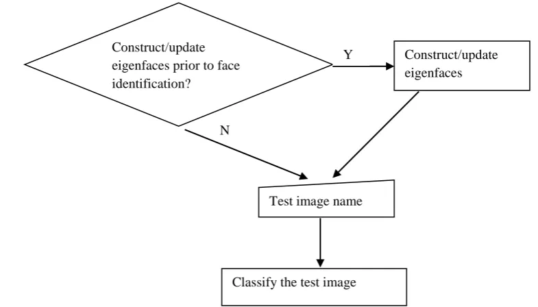
‗ConstructEigenfaces‘ and ‗ClassifyNewface‘ functions to complete the face recognition task.

System Structure

The structure of the system is shown in Figure 1. In the figure, the square shape indicates functions, and the parallogram represents files. An arrow pointing out from a file to a function means the function loads the file; an arrow pointing in the other direction indicates that the function creates or updates the file; a bidirectional arrow means the file is first read by the function, and later modified or updated

by it. These files help the

‗ConstructEigenfaces‘ and ‗ClassifyNewface‘ functions communicate with each other in a well organized way.

ConstructEigenfaces

ClassifyNewface

eigenfaces.mat

faceclasses.mat

note_eigenfaces.mat undoUpdateEigenfaces

LoadImages

(19)

Figure 1. System Flowchart. The squares and parallograms represent functions and files respectively. An arrow pointing out from a file to a function means the function reads/loads the file; an arrow pointing in the other direction indicates that the function creates/updates the file; a bidirectional arrow means the file is first

read by the function, and later

modified/updated by it. These files help the ‗ConstructEigenfaces‘ and ‗ClassifyNewface‘ functions communicate with each other in a well organized way.

Functional Blocks

Each functional block has a corresponding .m file (refer to the source code). Detailed description of the functional blocks is as follows.

LoadImages(imagefilename):

 Functionality: load all training images and return their contents (intensity values)

 Input parameters: imagefilename—a

string that states an image file name.

 Output parameters: I—a 3D matrix whose

components are the intensity values of the

training images.

 Use: I=LoadImages(imagefilename)

 Pseudo-code:

if imagefilename is an empty string

do

(1) read all default training images into 3D matrix I

(2) save I to file

‗trainingimages.mat‘ in ‗.\TrainingSet‘

directory (note: relative path is used throughout the document, ‗relative‘ in the sense that relative to the location of the .m source files)

(3) write the file names of the

default training images to text file

‗note_eigenfaces.txt‘ in ‗.\Eigenfaces‘