Article
1
Correlation between intense Solar Energetic Particle
2fluxes and atmospheric weather extremes
3G. Anagnostopoulos, S.A. Menesidou, V.G. Vassiliadis and A. Rigas 4
Department of Electrical and Computer Engineering, Democritus University of Thrace 5
* Correspondence: [email protected] 6
7
Abstract: In the past two decades the world experienced an exceptional number of unprecedented 8
extreme weather events, some causing major human suffering and economic damage, such as the 9
March 2012 heat event, which was called “Meteorological March Madness.” From the beginning of 10
space era a correlation of solar flares with pressure changes in atmosphere within 2-3 days or even 11
less was reported. In this study we wanted to test the possible relation of highly warm weather 12
events in North-East America with Solar Energetic Particle (SEP) events. For this reason we 13
compared ground temperatures TM in Madison, Wisconsin, with energetic particle fluxes P 14
measured by the EPAM instrument onboard the ACE spacecraft. In particular, we elaborated case 15
events and the results of a statistical study of the SEP events related with the largest (Dst ≤−150nT) 16
Coronal Mass Ejection (CME)- induced geomagnetic storms, between with the years 1997 – 2015
.
The 17most striking result of our statistical analysis is a very significant positive correlation between the 18
highest temperature increase. ΔTM and the time duration of the temperature increase ΔTM (r = 0.8, p 19
<0.001) at “winter times” ( r = 0.5, p , 0.01 for the whole sample of 26 SEP examined events). The time 20
response of TM to P was found to be in general short (a few days), but in the case of March 2015, 21
during a gradual P8 increase, a cross-correlation test indicated highest c.c. within 1 day (p < 0.05). 22
The March 2012 “meteorological anomaly” was elaborated in the case of South-East Europe, where, 23
beside a period of strong winds and rainfall (6-13.3.2012), intense precipitation in North-East Greece 24
(Alexandroupoli) were found to be correlated with distinct high energy flux enhancements. A rough 25
theoretical interpretation is discussed for the space – atmospheric extreme weather relationship we 26
found. However, much work should be done to achieve early warning of space weather dependent 27
extreme meteorological events. Such future advances in understanding the relationships between 28
space weather and extreme atmospheric events would improve atmospheric models and help 29
people’s safety, health and life. 30
Keywords: Extreme Weather events, Heat waves, Sun-Earth relationships, Sun and Weather, Space 31
Weather and Extreme Atmospheric events, Global Atmospheric Anomalies, SEP events and 32
Weather, SEP and NAO, Gulf Stream and Heat waves. 33
34
1. Introduction 35
“A growing mass of evidence suggests that transient events on the Sun affect our weather and 36
long-term variations of the Sun’s energy output affect our climate. Solar terrestrial exploration can 37
help establish the physical cause and effect relationships between solar stimuli and terrestrial 38
responses. When these relationships are understood science will have an essential role for weather 39
and climate prediction.” This statement was a part of an early proposal of R.D. Chapman submitted 40
to NASA [1]. This statement gains new interest nowadays, since in the past two decades we saw an 41
exceptional number of unprecedented extreme weather events, some causing major human suffering 42
and economic damage [2]. 43
Since the beginning of the space era, and, in particular, during the last two decades, an amount 44
of evidence has been gathered on links between Solar activity and variations in the Earth’s ionosphere 45
and atmosphere. 46
There are many reports from the beginning of space era suggesting a correlation of solar flares 47
with pressure gradients in the atmosphere, within 2-3 days or less (<6h) [3, 4, 5, 6, 1, 7, 8, 9]. In the 48
last two decades, great emphasis has been given to the solar cycle climate trends of cloudy, 49
stratospheric changes, polar temperatures and winds, as well as the sea and surface temperatures. 50
Most of these meteorological variations have been discussed in terms of solar irradiance as a stimuli, 51
but recently it suggested that energetic particle forcing driving dynamical changes in the atmosphere 52
are as intense as those arising from the solar irradiance variations [10]. In these studies, the solar 53
particles were considered to affect the atmosphere via a slow process of catalytic ozone destruction. 54
However, the question on the relationship between Solar Energetic Particle events and 55
atmospheric weather variations, in particular, with the extreme ones, is still open. 56
It is worth noting that the historic March 2012 heat wave was not anticipated by solely 57
atmospheric models. For instance, it has been noted that “A black swan most probably was 58
observed in March 2012”. Since, in March 1910, before the GHG era, similar temperatures were 59
recorded with those in March 2012, several scientists agree that the “Meteorological 2012 March 60
Madness” should be explained by physical and not anthropogenic agents. However, no convincing 61
new suggestions have been proposed to explain the March 2012 heat wave in USA and other extreme 62
events over the globe, within the framework of meteorological models, so far. 63
In a previous study we suggested that solar and magnetospheric particle events are consistent 64
with a cause of the extreme atmospheric weather events all over the globe, and in particular, the 65
historic March 2012 heat wave in East USA/Canada [4]. [4] noted that a great CME (March 7, 2012) 66
and a related geomagnetic superstorm were followed by various extreme phenomena as high 67
temperatures, intense rainfalls and ice extent at middle and high latitudes were recorded all over the 68
globe (USA, Europe, Australia, Antarctic), while unusual measurements of various atmospheric and 69
ionospheric quantities were observed by a series of satellites (TIMED, MODIS, NOAA etc.). 70
Therefore the question is: What are the primary physical processes that make an event extreme? 71
Is it possible for the Solar Energetic Particle (SEP) to provoke extreme weather events, like heat 72
waves? By which mechanism? Addressing this question is crucial to understanding the causes of 73
extreme events and to assess potential predictability. The answers are important for providing early 74
warning of extreme weather events. 75
In this paper we extend the case study by [4] to a statistical analysis on the possible relationship 76
of strong SEP events with extreme temperature increases. For this reason we present results from a 77
statistical study based on the selection of the strongest (Dst ≤−150 nT) interplanetary coronal mass 78
ejections (ICMEs) observed from the beginning of the life of ACE spacecraft in 1997 until May 2015. 79
A comparison of the space and atmospheric events during the times of the selected ICMEs suggests 80
a correlation between the strong ICMEs-related SEP events and temperature increases in north-east 81
USA (Madison, Wisconsin). Other atmospheric extreme phenomena on the globe were also found to 82
counteract the March 2012 heat wave in USA (and other SEP periods examined), but here we only 83
make a short reference to rainfall and strong winds in Greece (during March 2012). 84
85
2. Data 86
In order to check the possible link between the high solar activity and atmospheric extreme events, 87
we selected time periods with SEP events related with strong storms / superstorms. For the selection 88
of very strong geomagnetic storms we demanded geomagnetic Dst index values as low as Dst ≤−150nT, 89
and we examined the period from the beginning of the ACE mission (1997) until May 2015. Such large 90
(Dst ≤−150nT) storms are known to be caused by strong ICMEs [11]. By using a catalogue of CMEs 91
[http://www.srl.caltech.edu/ACE/ASC/DATA/level3/icmetable2.htm], we found only 28 SEP events 92
meeting the above criterion for large (Dst ≤−150nT) related geomagnetic storms within about 18 years 93
#6 & #22, which were put in brackets). Ιt is noted that, agreement with previous results [11] the majority 95
of the large ICME-induced storms were recorded during the maximum phases of solar cycles 23 and 24 96
(18 out of the total of 28 events). 97
Then we investigated the possible correlation of the SEP events observed by ACE with various 98
atmospheric parameters (temperature, wind, precipitation), around the times of the CME-related 99
storms. In some cases we checked the status of the atmospheric environment with data from MODIS 100
(Moderate Resolution Imaging Spectroradiometer) instrument onboard the TERRA satellite. 101
ACE (Advanced Composition Explorer) is a spacecraft (http://www.srl.caltech.edu/ACE/), 102
which has been circulating, around the L1 Lagrangian point; L1 is the point of Earth-Sun gravitational 103
equilibrium at a distance of ~220 RE, from Earth, where RE is the length of Earth’s radius. ACE was 104
launched on August 25, 1997 from the Kennedy Space Center in Florida and has been continuously 105
providing in situ observations until now. The ACE scientific research instrumentation includes eight 106
instruments that measure plasma and energetic particle composition, as well as one to measure the 107
interplanetary magnetic field (Stone et al. 1990) . 108
When reporting space weather, ACE provides an advance warning (about 1 hour) of 109
geomagnetic storms. Real-time observations with 1 second resolution are provided continuously to 110
Space Environmental Center (SEC) of the National Oceanographic and Atmospheric Association 111
(NOAA). For the present study we used data from the ACE Level 3 Summary Plots 112
(http://www.srl.caltech.edu/ACE/ASC/DATA/level3/summaries.html).In particular, for the needs of 113
our study we used the data from the EPAM (Electron, Proton, and Alpha Monitor) particle 114
instrument (http://sd-www.jhuapl.edu/ACE/EPAM; 115
[http://www.srl.caltech.edu/ACE/ASC/level2/lvl2DATA EPAM.html]. 116
In the next section we provide measurements from the channels P΄2 (ions), P8 (ions) DE1 117
(electrons) from the LEMS120, LEFS150 and LEMS30 telescopes of the EPAM instrument, 118
respectively; the numbers of these telescopes designate the angular orientation in degrees (150, 120 119
and 30) from the center of each channel with respect to the spacecraft spin axis which is always 120
pointed towards the Sun (Gold 1998). Since the vast majority of the ions measured are protons, we 121
call the ion measurements in the next section “proton” measurements. The three EPAM /ACE 122
channels P΄2, P8, and DE1 were chosen in order to compare the atmospheric weather with low energy 123
(~70-115 keV) protons (P2’), high energy (1880-4700 keV) protons (P8) and energetic (~40-50 keV) 124
electrons. The long time (days) structures of the P8 high energy ions are of solar origin; spikes of low 125
energy P2’ protons and DE1 electrons are originated from the Earth’ s magnetosphere [13]. 126
Ground data of atmospheric temperature, precipitation and wind direction were obtained from 127
the WeatherOnline site (http://www.weatheronline.co.uk/weather/). 128
129
3. Data analysis 130
The set of 26 time intervals with the largest (Dst ≤−150nT) CME- induced geomagnetic storms 131
during the time period of ~18 years (1997-2015) was examined in order to compare the SEP events 132
with possible significant weather events. We compared the SEP events observed by the ACE 133
spacecraft with the atmospheric weather at various sites over the globe and the most important 134
conclusions of our investigation were (a) an evidence for significant or even great temperature 135
increases during winter times in North-East USA and (b) a less significant trend for rainfalls and 136
other “winter” weather conditions in Greece. A preliminary investigation of the whole set of 26 SEP 137
events and the weather at various sites of Earth suggests that at least in some cases, as for instance, 138
March 2012, the SEP events were related with global atmospheric weather extremes. 139
In subsection 3.1 we show representative observations, where three SEP events are compared 140
with the atmospheric weather conditions in Madison, Wisconsin. In subsection 3.2 we present the 141
results from a statistical study on temperature variations in Madison during the 26 large storms. 142
Finally, in subsection 3.3 we provide data and published information for the March 2012 large SEP 143
In order to provide information for each of the 26 periods examined we show in Table I the date 145
of the onset of the high energy proton P8 and the corresponding temperature in Madison Tias well as 146
the date Tf when the temperature in Madison takes its maximum value. We also show the time 147
difference ΔΤ = Tf- Ti, the time period Δτ (in days) between the dates with Ti and Tf. as well as the 148
lowest value of the index Dst corresponding to the selected geomagnetic storm. 149
Table 1. Date of a SEP onset and the corresponding temperature in Madison, maximum temperature in 150
Madison and the corresponding date, temperature increase and its corresponding time duration along 151
with the lowest value of the index Dst of the selected geomagnetic storm 152
Year Month Day (TI) TI Day (TF) TF Δτ ΔΤ Dst
1 1998 9 24 (267) 17 26(269) 29.5 2 12.5 -207
2 1998 8 27 (239) 25 29(241) 28.5 2 3.5 -155
3 1998 5 3 (123) 3 4(124) 23 1 20 -205
4 1999 10 17 (290) 9 21(294) 19 4 10 -237
5 1999 9 21 (264) 15 26(269) 28 5 13 -173
[6] 2000 11 9 (314) 2 12(317) 6 3 4 -159
7 2000 10 6 (280) 6 10(284) 17 4 11 -182
8 2000 9 15 (259) 16 18(262) 29 3 13 -201
9 2000 8 5 (218) 22 14 (227) 29 9 7 -235
10 2000 7 12 (194) 26 13 (195) 29 1 3 -301
11 2000 4 4 (95) 7 5 (96) 14 1 7 -288
12 2001 11 20 (324) 6 24 (328) 16 4 10 -221
13 2001 11 5 (309) 14 6 (310) 19 1 5 -292
14 2001 10 25 (298) 3 28 (301) 14 3 11 -157
15 2001 10 16 (289) 9 22 (295) 17 6 8 -187
16 2001 4 15 (105) 1 11 (101) 23 -4 22 -271
17 2001 3 25 (84) -6 30 (89) 10 5 16 -387
18 2002 10 7 (280) 10 11 (284) 23 4 13 -146
19 2002 9 3 (246) 26 8 (251) 32 5 6 -181
20 2003 11 19 (323) 12 20 (324) 18 1 6 -422
21 2003 10 26 (299) 7 30 (303) 18 4 11 -353
[22] 2004 11 8 (313) 5 10 (315) 17 2 12 -263
23 2004 7 24 (206) 22 27 (209) 28 3 6 -170
24 2005 8 22 (234) 21 27 (239) 29 5 8 -216
25 2005 5 12 (132) 10 22 (142) 25 10 15 -247
26 2006 12 7 (341) -8 14 (348) 11 7 19 -162
27 2012 3 4 (64) -2 15(75) 28 11 30 -145
28 2015 3 5 (64) -9 16(75) 23 11 32 -222
153
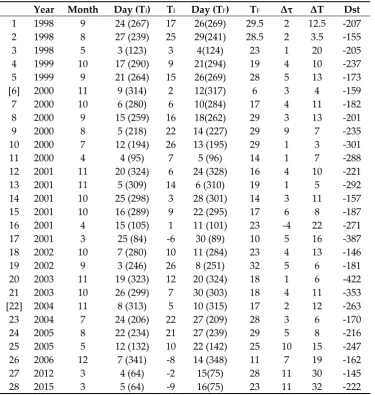
Figure 1 shows time profiles of the daily maximum value of temperature TM in Madison, 154
Wisconsin (panel a), the direction of the wind in the same town (panel b), the fluxes of energetic (38-155
53 keV; DE1 channel) electrons, and of both the low (68-115 keV; P1 channel) and the high (1880-4700 156
keV; P8 channel) energy protons observed by the spacecraft ACE outside the Earth’s magnetosphere 157
(panel c) along with the geomagnetic index Dst (panel d), for the time period March 3-31, 2015; the 158
time series of Figure 1 have been centered around the time of the severe (G4) storm of March 17 which 159
was triggered by the most intense CME of the solar cycle 24 (Dst index reached values as low as -223 160
nT on day 17). 161
By comparing the profiles of the ACE energetic particle flux profiles (panel c) with the profile of 162
temperature TM (panel a) we see a gradual increase of both P8 flux and TM values from day 6 until 163
day 16 (the day before the CME arrival), and a decrease of both TM and P8 from 17 to 28 March, 2015. 164
within 10 days (6-16.3.2012) or 3.20C / day for 10 days. This temperature variation means a change 166
from a winter-type weather (-90C) to a summer-type one (230C) in the beginning of March 2015. 167
From Figure 1, we also see a better correlation of the high energy proton flux than of the low 168
energy proton and electron flux with the temperature TM (in particular during the arrival times of 169
high energy solar protons between 6-16 March). The short lived spikes of low energy protons are 170
obviously of a terrestrial origin (magnetosphere, bow shock) and their presence is evident throughout 171
the geomagnetic storm, in particular between days 17-25. From these observations we can infer that 172
the long lived and great temperature increase during March 2015 was related with the SEP event and 173
not with the highly activated magnetosphere. An increase of DE1 electron flux was also observed 174
during the maximum of the SEP event, as inferred from the P8 flux-time profile, between days ~15-175
16. 176 177
178 179
Figure 1: Time profiles of temperature in Madison, Wisconsin (panel a), the direction of wind in the same 180
town (panel b), the fluxes of energetic proton and electrons observed by the ACE spacecraft and (d) the 181
values of the geomagnetic index Dst, during March 3-31, 2015. It is evident that the temperature profile 182
(panel a) resembles that of the high energy solar proton flux P8 (red curves). In particular, we note that 183
the great temperature increase from -90C to 230C, between 6-16.3.2015 (panel a), was recorded under a 184
general south wind streaming (panel b). 185
186
Further comparison between panels a, b and c demonstrates that during the time of the gradual 187
increase of energetic protons at ACE and the temperature in Madison, the wind shows a general flow 188
from the southward direction (days 6-16; panel b). On the contrary, we see that before day 6 (days 4-189
5) and after day 16 (days 17-19), both the P8 proton flux and the temperature TM in Madison show 190
192 193
194 195
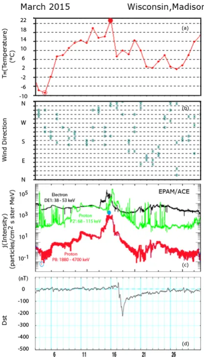
Figure 2: The estimates of the cross-correlation coefficients r for lags k = 0;±1;…;±7, between the daily 196
values of the logarithm of the P8 proton flux values and the temperature TM from day 6 until day 16, 197
March 2015. The solid black lines present the asymptotic 95% confidence limits of the estimated 198
coefficients. The very large r value at lag=0 confirms and explains the good resemblance of P8 and TM
199
curves seen in Figure 1. 200
201
In Figure 2 we present the estimates of the cross-correlation coefficients between the logarithm 202
of the P8 proton flux values and the temperature TM from day 6 until 16 (Fig. 1) and for lags 0, ±1,..., 203
±7. The upper and lower confidence limits are denoted with solid black lines. We found a very 204
significant positive correlation at lags -1, 0 and 1. Especially at lag = 0 the cross-correlation coefficient 205
takes its maximum value r = 0.907 with s.e.= 0.277(p <0.001). This indicates that one should notice an 206
increase of the temperature TM from the previous day till one day after an analogous increase of the 207
proton flux. The very large r value, at lag = 0, confirms and explains the day to day simultaneous 208
resemblance of the line plots of the temperature TM and the P8 proton flux in Figure 1. The significant 209
level of the correlation is better than 0.001, which suggests a very significant correlation between the 210
two magnitudes (TM and the P8), or between space weather and atmospheric weather in Madison. 211
The very strong and significant correlation between the temperature in Madison during a time 212
interval of ~10 days before the occurrence of the geomagnetic superstorm suggests that the change of 213
weather in Madison may be causally dependent to the SEP event. 214
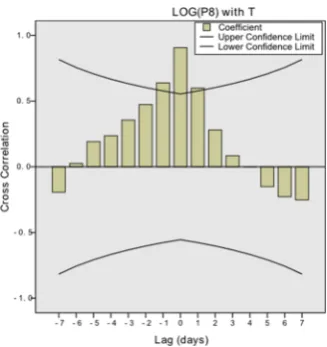
Figures 3 and 4 have been constructed as Figure 1, but at times around the superstorms of 215
December 2006 (Figure 3) and September 2002 (Figure 4).The data set in these two figures show 216
similarities with each other and with the data examined in Fig. 1. The large structures of energetic 217
particle fluxes (panels c) between dates 6-20.12.2006 (Figure 3) and 6-16.2002.2002 (Figure 4) are 218
obviously of solar origin. There are also some differences. In both cases, the solar events show a rather 219
abrupt flux increase in all of the three channels (DE1, P2’, P8) in contrast to the solar event of March 220
2015 (Figure 1). These profiles suggest a rather good magnetic connection of the ACE / Earth with the 221
corresponding solar source. After the SEP maximum, the DE1, P2’ and P8 fluxes display a gradual 222
decay, with several low energy P2’ proton spikes of a terrestrial origin [13]. 223
The most important common feature of the great CME-SEP events in December 2006 and 224
September 2002 is a significant temperature increase (panel a) during times of highest solar particle 225
fluxes and a general south wind streaming (panel b). However, there is a remarkable difference in 226
the solar events in December 2006 and September 2002. During the “winter” event of December 2006, 227
the temperature TM climbs from -70C to 110C, that is an increase ΔTM,= 190C, within only 7 days, 228
Figure 3. As in Figure 1 but for the SEP events related with the December 2006 (left side) and September 2002 (right 230
side) ICME-induced great storms. The temperature increase TM in Madison (Wisconsin) was much greater (panel 231
a) in December 2006 (ΔΤ = 190C) than in September 2002 (ΔΤ = 40C) during a south wind, bur under different pre-232
event temperatures (-80C versus 40C). 233
234
which resembles the great change from winter to summer weather in Madison in March 2015 (Figure 235
1). On the contrary, the increase of the temperature TM was much lower in September 2002, with an 236
increase from 280C to 320C, that is a total increase of only 40C, in the same town, but under a very 237
high pre-event temperature level (~280C compared to -80C in December 2006 and -90C in March 2015). 238
It worth noting that this difference in the TM variation under a different pre-event temperature level 239
(“summer” –“winter” asymmetry) was found to be a characteristic statistical significant result in the 240
sample of 26 events examined, as we will see in the next subsection 2.3. 241
In addition, we note that in the cases of SEP events of December 2006 and September 2002 with 242
abrupt flux increases, the TM temperature does not show such a strong and significant correlation 243
with P8 flux as in the case of gradual flux increase in March 2015. This may suggest that the 244
troposphere follows well the progress of SEP events during a slow external stimuli. 245
3.2. Statistical Results on temperature increases in Madison, Wisconsin (USA) 246
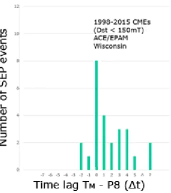
Figure 5 shows the distribution number of the 26 SEP events with a time delay ∆τ (=TM - P8) 247
between the day of the maximum temperature TM in Madison and the day of the maximum solar 248
proton flux P8, within a time interval of 15 days centered on the day of the ICME arrival. Positive 249
(negative) values of delay time ∆τ means later (earlier) recording of maximum temperature TM in 250
Madison than that of the maximum solar flux P8. From Figure 5 we see that the majority of events 251
show non-negative values, which suggest that maximum surface temperature either coincides with 252
(∆τ = 0) or follows (∆τ >0) the proton maximum P8. 253
255
256 257
Figure 4: Distribution number of SEP events with time lag Δt between the day of maximum temperature 258
TM in Madison and the day of maximum high energy solar proton flux P8 during a period of 15 days 259
centered at the day of the ICME (=0 at the horizontal axis). The large number of non-negative values 260
suggests that the maximum temperature TM coincides with or follows the day of solar proton maximum. 261
262
In Figure 5 we present scatter plots of the total temperature increases ∆TM versus the time 263
duration Δτ of the temperature increase, for winter times (October to April; panel a) and for summer 264
times (May - September; panel b), respectively. Panel a shows a very strong correlation (r = 0.8), 265
between ∆TM and ∆τ, which is very significant (p <0.001). A linear interpolation shows a trend b = 266
2.026, which suggests an average daily temperature increase ∆TM / ∆τ ≈ 20C / day at winter time 267
periods in Madison, during the SEP events related with very large (Dst ≤−150nT) storms. From panel 268
b we infer the absence of a significant correlation between ∆TM and ∆τ during the “summer times”. 269
Furthermore, from a comparison of the data in panels a and b, we infer that the SEP events examined 270
are related with lower temperature increases ∆TM in “summer” times (panel b) than in “winter” times. 271
This finding is a reasonable result for an external stimuli of the atmospheric circulation. 272
When all of the 26 events are considered (panel c) a significant correlation was also found 273
between ∆TM - ∆τ (r = 0.5, p<0.01). 274
The statistical results of Figure 4 and 5, that is the occurrence of high temperatures in Madison 275
TM after the maximum flux of CME-related high energy protons P8 and the very strong and 276
significant correlation between TM and P8 during “winter times” suggest that most probably there 277
exists some physical causality between SEP events and atmospheric weather in North-East USA 278
(Madison / Wisconsin). 279
281 282
Figure 5: Surface temperature increase ΔT during SEP events as a function of the time duration Δτ of 283
the temperature increase, during “winter” (a) and “summer" times (b). During “winter times", a strong 284
and very significant (r = 0.8; p <0:001) correlation was estimated. 285
286
3.4. SEP events and global atmospheric extremes (March 2012) 287
From the previous analysis of space and meteorological events during times of 26 selected 288
ICME-related SEP events (1997-2015) we inferred a correlation between the strong ICME-related solar 289
energetic (>~2-5 MeV) proton fluxes and the temperature increases in north-east USA (Madison, 290
Wisconsin) during “winter” times. Other atmospheric anomalies were also found to follow the SEP 291
events over the globe, but here we only make a short reference to the extreme weather event in South-292
East Europe following the March 2012 CME. 293
Here we concentrate on the comparison of CME-related SEP event observed by ACE with the 294
atmospheric weather extreme in two cases: the north–east USA (Figure 6, left side) and Greece (Figure 295
6, right side). 296
Figure 6 has also been constructed as Figure 1. Figure 6-left side compares the EPAM / ACE 297
electron and proton observations with temperature and wind stream direction in Madison / 298
Wisconsin, between 3-30 March 2012, while Figure 6-right side compares the same ACE observations 299
with temperature and precipitation in Alexandroupoli / North Greece, for the same time period. 300
A SEP structure is obvious in EPAM / ACE data between 4-17.3.2012 and a smaller one between 301
28-30.3.2012. The flux enhancement on 5th of March is related with the appearance on the solar disk 302
of solar active region (AR) 11429 of the National Oceanic and Atmospheric Administration (NOAA). 303
[14]. 304
The solar flares in March 2012 were analyzed and discussed in extent in the scientific literature 305
[14]. The most intense UV flash of X5-class solar flare occurred on March 7, 2012. This flare was 306
associated with a very intense CME with a speed of ~2000 km s−1.The impact of the 2012 March 7 solar
307
eruptions in the heliosphere and the geospace was striking [15, 16]. Noteworthy is a very strong 308
Furthermore, significant substorm activity was detected in geosynchronous equatorial orbit (GEO) 310
by GOES-13 and 15, in particular on 2012 March 9, during the major geomagnetic storm. [14]. 311
312
313
Figure 6. As in Figure 1 but for the SEP events related with the March 2012 ICME-induced great storm, 314
in Madison, Wisconsin (left side) and Alexandroupoli, Greece (right side). The temperature increase 315
TM in Madison reached an historic maximum, with a change from -20C to 280C, that is ΔTM = 300C,
316
within 10 days (6-16.3.2012), which is not explained by the existing atmospheric models (see in text). 317
Figure 6-right side shows a general anticorrelation between the P8 high energy proton flux and the 318
temperature in Alexandroupoli / Greece, with three time intervals with rainfall in Alexandroupoli 319
(blue bars in panel b) at times of enhanced levels of high energy proton P8 flux (around days 8, 14, and 320
30 of March 2012). The inset in the left side shows the precipitation amount evaluated by the MODIS 321
instrument onboard the TERRA satellite on March 8. The different weather in North-East USA and 322
North Greece reflects a global weather anomaly in March 2012 (See Figure 8) during the SEP event. 323
324 325 326
From Figure 6 we see that there was an increase in the temperature in Madison TM (panel a) after 327
the arrival of solar energetic particles on 4th of March (panel c), while the wind was streaming from 328
the southward direction (panel b). The temperature TM, showed a dip for two days (8-9.3.2012), while 329
the wind was streaming from the northward direction, but it continued its gradual increase from day 330
10 to day 16. 331
From Figure 6 we see that there was an increase in the temperature in Madison TM (panel a) after 332
the arrival of solar energetic particles on 4th of March (panel c), while the wind was streaming from 333
the wind was streaming from the northward direction, but it continued its gradual increase from day 335
10 to day 16. 336
The temperature TM remained at high levels of ~26-280 C for ~7 days, until day 21, under air 337
streams from the southward direction, and then started to decrease; it is pointed out that the TM 338
increased from -20C to 280C, that is ΔTM = 300C, within 10 days (6-16.3.2012). This huge temperature 339
variation in Madison reflects a general temperature increase over large regions of North-East 340
America, and is known as an “historic heat wave”, which brought the summer in winter times. 341
On the contrary, in Figure 6-right side we see a general anticorrelation between the P8 high 342
energy proton flux during the period of the main SEP event (5-20.3.2012) and the temperature in 343
Alexandroupoli / Greece. In addition, three time intervals with rainfall in Alexandroupoli (blue bars 344
in panel b) are seen at times of enhanced levels of high energy proton P8 flux (around days 8, 14, and 345
30 of March 2012). Actually there existed extreme weather conditions in Greece with strong rainfalls, 346
snowfalls and strong winds… The inset in Figure 8 shows the precipitation amount evaluated by the 347
MODIS instrument onboard the TERRA satellite on March 8, with high values in Greece and 348
Southern Italy; it is remarkable that, at the same time, Western and Central Europe experienced one 349
of the warmest months of March on record [18]. 350
What is of particular interest for the March 2012 events is the detection of very high energy 351
protons from PAMELA (data not shown here). PAMELA is a magnetic spectrometer launched into a 352
near-Earth orbit in June 2006. Among the goals of the high-energy charged particle measurements 353
fulfilled by the PAMELA spectrometer is the observation of particle fluxes enhancements after a 354
sudden energy release at the Sun (SEPs). [19]. PAMELA observed high fluxes of >200 MeV protons 355
between 7-15.3.2012 and even >500 MeV protons between 7-9.3.2012 and 14-15.3.2012 [19, Fig. 1]. 356
Moreover, the increase of >500 MeV proton flux by ~2 orders of magnitude suggest the presence of 357
protons of even higher energies (>>500 MeV). [20] found that an intensification of zonal circulation 358
took place due to the >100 MeV SEP increases, which is able to affect directly the lower atmosphere 359
by changing its thermal state. The incident of >>500 MeV protons in the Earth’ atmosphere may 360
produce ionization in the troposphere. 361
6. Conclusions and Discussions 362
6.1 Space weather (SEP) and extreme atmospheric weather events between the years 1997 - 2015 363
The influence of space weather on the Earth’s atmospheric weather and climate is an important 364
scientific issue with great social interest. Ιn the past two decades we saw an exceptional number of 365
unprecedented extreme weather events, which caused major human suffering and economic damage. 366
Understanding the causes of extreme weather is of great importance to assess potential predictability 367
and provide early warning. 368
In the last two decades, great emphasis has been given to long term space (solar cycle) dependent 369
climate changes, but not to possible short time solar effects on atmospheric weather. Significant 370
evidence from early studies (<1990) suggesting a short response of the troposphere to Solar Energetic 371
Particle (SEP) events, has not attracted significant investigation. 372
In this study we present statistical results from a sample of 26 large ICMEs-induced great (Dst ≤
373
−150nT) geomagnetic storms between the years 1997 - 2015, which suggest a strong correlation of 374
space weather with the temperature TM in North-East USA (Madison, Wisconsin). 375
In particular we found that: (a) during a time period of 15 days (day=-7 to day=+7) centered at 376
the day D0 of ICMEs arrival at Earth, the temperature (TM) in Madison shows maximum values, in 377
~89% of the events examined, not earlier than the day D0, , (b) the high (P8: 1880 - 4700 keV) energy 378
solar proton fluxes P8 show a much better relation with TM than the magnetospheric (68-115 keV) ions 379
and )38 - 53 keV electrons), (c) the temperature increase ΔTM reached is very strongly and significantly 380
correlated with the time duration of the high energy (P8) protons and the corresponding duration Δτ
temperature increase (r = 0.8, p <0.001), (d) the temperature increase ∆TM during the high energy 382
proton events shows an average rate of ∼ 2◦C/day (26 events examined), (e) (d) in some case examined 383
warm air flowing from the southward direction were found to be related with the high energy proton 384
flux and the temperature increase, and (f) the temperature TM was very strongly and significantly 385
correlated with the P8 proton flux during the gradual P8 SEP increase of March 2015, within ∼ 1 day 386
(r = 0.9, p <0.001).
387
From the above results we infer that the SEP events preceding the great ICME-related 26 great 388
storms, between the years 1997 – 2015, strongly controlled the temperature TM in eastern USA, in 389
particular, during the “winter” times. A second result implied from several SEP periods we 390
investigated is that the temperature increase in Madison was related with wind streaming from the 391
southward direction. 392
Among the SEP periods examined between the years 1997 – 2015, one case coincides with the 393
well known March 2012 historic heat wave in North America. During March 2012 the highest 394
temperature in North America was recorded since 1910. NASA has posted an image on “Earth 395
Observatory” entitled “Historic Heat in North America Turns Winter to Summer”, which is 396
presented in Figure 7. 397
398 399
400
401 402
Figure 7. March 8 - 15, 2012 Land Surface Temperature anomaly in North America. (This NASA Earth 403
Observatory image was provided by Jesse Allen, using data from the Level 1 and Atmospheres Active 404
Distribution System (LAADS) and was captioned by Adam Voiland
405
(https://earthobservatory.nasa.gov/images/77465/historic-heat-in-north-america-turns-winter-to-406
summer). 407
408
Moreover, March 2012 was not only a local historic record of warm weather in North America, 409
but a global meteorological anomaly. Various extreme phenomena such as high temperatures, 410
intense rainfalls and ice extent at middle and high latitudes followed the March 7, 2012 CME all over 411
the globe (USA, Europe, Australia, Antarctic), while unusual measurements of various atmospheric 412
and ionospheric quantities were observed by a series of satellites (TIMED, MODIS, NOAA etc.) 413
Selected Weather anomalies all over the globe have been noted by the NOAA “Global Climate Report 414
-March 2012 (https://www.ncdc.noaa.gov/sotc/global/201203); a NOAA map with such anomalies is 415
shown in Figure 8. The National Climatic Data Center (NCDC) preliminary data indicate that March 416
2012 had a global-mean temperature of 0.46°C above the twentieth-century average [21st]. 417
419 420
Figure 8. Global Climate Report by NASA for the March 2012 weather anomaly 421
(https://www.ncdc.noaa.gov/sotc/global/201203) 422
423 424
[18] in their study on the origin of the March anomaly state: “Nature’s exuberant smashing of 425
high temperature records in March 2012 can only be described as “Meteorological March Madness.” 426
The numbers were stunning”. This event was not anticipated by solely atmospheric models and it 427
was called a “black swan event” 428
(http://www.esrl.noaa.gov/psd/csi/events/2012/marchheatwave/anticipation.html). [18] also 429
concluded that observations and models are “in rough agreement in suggesting that a temperature 430
increase of up to approximately 1°C could be anticipated from the long-term warming trend, which 431
in the CMIP5 (Coupled Model Intercomparison Project) results is mostly due to external forcing from 432
increasing greenhouse gas concentrations. Compared to the observed peak event magnitude of 433
approximately 20°C, a 1°C increase is small”. 434
6.2 Space weather (SEP) and extreme atmospheric weather event relationship: Physical links? 435
The March 2012 historic heat waves, several extreme weather events experienced in the past two 436
decades, and the results of the present study pose the question of the possible mechanism(s) 437
mediating certain SEP events with major variations in the troposphere. 438
Several physical mechanisms have been proposed in order to explain some links between high 439
SEP events and solar magnetosphereric particle activity with changes in atmospheric conditions so 440
far. Such mechanisms include SEP relation with large stratospheric/tropospheric pressure gradient 441
causing downward air flow, variation in the global electric circuits and stratospheric ozone-related 442
chemical energy changes [1, pp. 174-181]. 443
Since our results in the present study indicated a fast correlation between the high energy proton 444
flux and the temperature TM in Madison (of the order of ∼ 1 day; Figure 2), the catalytic ozone 445
destruction, which is a slow process, must not be the major driver of the SEP related temperature 446
variation in north-east USA (Wisconsin). 447
Furthermore, the results of the present study suggest that the south air flow seems to mediate 448
the influence of SEP events with the surface temperature variations. Furthermore, we note that during 449
the great ICME of March 2015, the temperature TM increased from -90C to 230C (an increase of 32◦C), 450
within only 10 days (6-16 March 2015). These results support the concept of a very effective 451
mechanism by which SEP events can produce major tropospheric variations (at least heat waves in 452
North-East America). 453
The correlation of south wind streaming with the TM temperature increasing in Madison (and a 454
broad region in North-East America) during SEP events, most probably suggests a physical link 455
Although this hypothesis needs further examination, we note the following known physical 457
phenomena, which support such a concept: (1) a correlation between SEP activity and the North 458
Atlantic Oscillation (NAO) [21, pp250-255]., (2) a solar cycle periodicity of the Gulf Stream activity 459
[22], and (3) a correlation between NAO index and the sea surface temperature in the east USA [21]. 460
These results may suggest a physical link between SEP flux increase / NAO index variation / Gulf 461
stream intensification, south warm air flows and temperature increases in east USA. Finally, we note 462
the fast (within ∼ 1 day) response of TM to SEP events, which rather suggests that a non-linear process 463
controls the physical processes described above. Magnetospheric particle may also contribute in 464
weather variations during the large geomagnetic particle activity [10], while hard energy proton (>> 465
500 MeV) events may trigger global anomalies, as in the case of March 2012. 466
The present work generalizes the results presented in [23, 24]. 467
In concluding, the 26 Solar Energetic Particle (SEP) events observed by the ACE spacecraft 468
between the years 1997-2015 were found to be related with temperature increase in Madison, 469
Wisconsin, while some of them were related with global weather anomalies (including the March 470
2012 global anomaly). These results suggest that SEP events should be further investigated as a 471
possible agent of some extreme (global) weather phenomena. 472
473
Author Contributions: Conceptualization and Methodology, A.G.; Statistical analysis, V. V. G and R. A; Data 474
Processing and Analysis, M.S.A; Writing-Original Draft Preparation, A.G; Writing-Review & Editing, A.G. and 475
M.S.A. 476
477
Funding: This research received no external funding. 478
479
Acknowledgments: The authors thank Dr L. Lanzerotti for providing the ACE / EPAM energetic particle data 480
and they acknowledge the use of meteorological data from WeatherOnline Online Services and geomagnetic 481
data from the World Data Center for Geomagnetism, Kyoto. The authors also acknowledge the ICME list 482
provided by Dr Ian Richardson. 483
Conflicts of Interest: Declare conflicts of interest or state “The authors declare no conflict of interest.” 484
References 485
[1] Herman, J. R. & Goldberg, R. A., Sun, weather, and climate, Dover Pub. Inc., New York, 1978 486
[2] Coumou D. and St. Rahmstorf, A decade of weather extremes, Nature, 2012, DOI: 10.1038/NCLIMATE1452 487
[3] Cobb, W. E., Evidence of a solar influence on the atmospheric electric elements at Mauna Loa Observatory. 488
Man. Weather Rev., 1967, 95, 12, 905-911. 489
[4] Schuurmans, C.J.E.; Oort, A.H. A statistical study of pressure changes in the troposphere and lower 490
stratosphere after strong solar flares. PAGEOPH1969, 75, 1, pp. 233–246. 491
[5] Schuurmans, C. J. E. The influence of solar flares on the tropospheric circulation. (Statistical indications, 492
tentative explanation and related anomalies of weather and climate in Western Europe). Publisher: 493
Staatsdrukkerij, 1969. 494
[6] Reiter, R. Increased influx of stratospheric air into the lower troposphere after solar Hα and X ray flares. J. 495
Geophys. Res. 1973, Volume 78, pp. 6167-6172. 496
[7] Schuurmans, C. J. E. Tropospheric Effects of Variable Solar Activity. Sol Phys, 1981, 74, 2, 417-419. 497
[8] Gray, L. J., J.; Beer, M.; Geller, J. D.; Haigh, M.; Lockwood, K.; Matthes, U.; Cubasch, D.; Fleitmann, G.; 498
Harrison, L.; Hood, J.; Luterbacher, G. A.; Meehl, D.; Shindell, B. van Geel W.; White, Solar influences on 499
Climate, Reviews of Geophysics, 48, 1-53, 2010. 500
[9] Avakyan, S.V.; Voronin, N.A.; Nikol’sky, G.A. Response of atmospheric pressure and air temperature to the 501
solar events in October 2003. Aeron, 2015, 55, 8,1180–1185. 502
[10] Seppala A., M.A. Clilverd, Energetic particle forcing of the Northern Hemisphere winter stratosphere: 503
comparison to solar irradiance forcing, Frontiers in Physics, 2, 25.6, 10.3389/fphy.2014.00025, 2014. 504
[11] Richardson I. G., Solar wind stream interaction regions throughout the heliosphere, Living Rev. Sol. Phys., 505
[12] Stone, E. C.; Burlaga, L. F.; Cummings, A. C.; Feldman, W. C.; Frain, W. E.; Geiss, J.; Gloeckler, G.; Gold, R. 507
E.; Hovestadt, D.; Krimigis, S. M.; Mason, G. M.; McComas, D.; Mewaldt, R. A.; Simpson, J. A.; von 508
Rosenvinge, T. T.; Wiedenbeck, M. E. The advanced composition explorer, Particle Astrophysics. AIP Conf. 509
Proc. 1990, 203, 48-57. 510
[12] Gold, R. E.; Krimigis, S. M.; Hawkins, S. E., III; Haggerty, D. K.; Lohr, D. A.; Fiore, E.; Armstrong, T. P.; 511
Holland, G.; Lanzerotti, L. J. Electron, Proton, and Alpha Monitor on the Advanced Composition Explorer 512
spacecraft, Space Sci 1998, Volume 86, 1/4, 541-562. 513
[13] Anagnostopoulos G. C., G. Kaliabetsos, G. Argyropoulos and E.T. Sarris, Upstream energetic (50-11 220 keV) 514
ion events associated with high energy electron (≥ 220 keV) and ion (≥ 290 keV) bursts: Six years (1982-1986) 515
statistical results, Geophys. Res. Lett., 1999, 26, 14, 2151. 516
[14] Patsourakos, S.; Georgoulis, M. K.; Vourlidas, A.; Nindos, A.; Sarris, T.; Anagnostopoulos, G.; Anastasiadis, 517
A.; Chintzoglou, G.; Daglis, I. A.; Gontikakis, C.; Hatzigeorgiu, N.; Iliopoulos, A. C.; Katsavrias, C.; 518
Kouloumvakos, A.; Moraitis, K.; Nieves-Chinchilla, T.; Pavlos, G.; Sarafopoulos, D.; Syntelis, P.; Tsironis, C.; 519
Tziotziou, K.; Vogiatzis, I. I.; Balasis, G.; Georgiou, M.; Karakatsanis, L. P.; Malandraki, O. E.; Papadimitriou, 520
C.; Odstrčil, D.; Pavlos, E. G.; Podlachikova, O.; Sandberg, I.; Turner, D. L.; Xenakis, M. N.; Sarris, E.; 521
Tsinganos, K.; Vlahos, L. The major geoeffective solar eruptions of 2012 March 7: comprehensive Sun-to-522
Earth analysis, Astrophys. J. 2016, 817:14, 1, 14, 19.01.2016. 523
[15] Lario, D.; Ho, G. C.; Roelof, E. C.; Anderson, B. J.; Korth, H. Intense solar near-relativistic electron events at 524
0.3 AU.J. Geophys. Res.Space Physics, 2013, 118, 63–73. 525
[16] Zeitlin, C.; Hassler, D. M.; Cucinotta, F. A.; Ehresmann, B.; Wimmer-Schweingruber, R. F.; Brinza, D. E.; 526
Kang, S.; Weigle, G.; Böttcher, S.; Böhm, E.; Burmeister, S.; Guo, J.; Köhler, J.; Martin, C.; Posner, A.; Rafkin, 527
S.; Reitz, G. Measurements of energetic particle radiation in transit to mars on the mars science laboratory. 528
Science, 2013, 340, 1080–1084. 529
[17] Papaioannou, A.; Souvatzoglou, G.; Paschalis, P.; Gerontidou, M.; Mavromichalaki, H. The First 530
Ground-Level Enhancement of Solar Cycle 24 on 17 May 2012 and Its Real-Time Detection, Solar
531
Phys. 2014, Volume 289, 423-436. 532
[18] Dole, Hoerling, Kiladis, Webb, Kumar and Chen, Eischeid, Perlwitz, Quan, Murray, Wolter,Zhang, The 533
making of an extreme event: Putting the Pieces Together, 2014, American Meteorological Society, 534
427,DOI:10.1175/BAMS-D-12-00069.1. 535
[19] Bazilevskaya G.A.; Mayorov A.G.; Mikhailov V.V. Comparison of solar energetic particle events observed 536
by PAMELA experiment and by other instruments in 2006-2012, Proceedings of the 33rd International 537
Cosmic Ray Conference, Rio de Janeiro, Brazil, 2013, 332. 538
[20] Pudovkin M. I. and S. V. Babushkina, The Influenceof Solar Flares and Disturbances of the interplanetary 539
medium on the Atmospheric Circulation, J. Atmos.Terr. Phys., 1992, 54 (7/8), 841–846. 540
[21] Benestad R.E., Solar Activity and Regional Climate Variations in Solar Activity and Earth’ Climate, 2002, 541
250-255. 542
[22] Taylor, H., North - South shifts of the Gulf Stream and their climatic connection with the abundance of 543
zooplankton in the UK and its surrounding seas, ICES Journal of Marine Science, 52, 711-721, 1995 544
[23] Anagnostopoulos G., Correlation between Space and Atmospheric March 2012 Extreme Events, Geophysical 545
Research Abstracts Vol. 17, EGU 2015-14048, http://presentations.copernicus.org/EGU2015-14048 546
presentation.pdf, 2015. 547
[24] Anagnostopoulos, G.; Menesidou, S.A.; Vassiliadis, V.; Rigas, A. Correlation between Solar Particles and 548