A New ELECTRE-II Approach Using Separation
Method And Grey Subjective-Objective Weights'
Allocation Scheme
Mohamed F. El-Santawy, Soha Mohamed
Abstract: This paper presents a new method called G-ELECTRE-II for dealing with MCDM problems contain grey data. The proposed approach employs the separation method for the first time in Grey MCDM in a novel way. The proposed method determines the most effective choice among all alternatives within the case of data is represented as grey numbers. The new approach contains a completely novel scheme to allocate grey weights supported by both grey subjective grey objective weights and therefore the geometric mean is allocated for mixing both grey weights.. A numerical example is presented for validation. The method shows its capability to deal with grey MCDM with no weights for criteria.
Keywords: ELECTRE-II, Grey numbers, Multi-Criteria Decision Making, Subjective weights, Separation method, Objective weights.
—————————— ——————————
1
INTRODUCTION
Our decisions are daily incorporating many conflicting aspects, features, points of views, and criteria in real life. The process to choose an alternative among set of choices is not easy when the relevant criteria of selection are contradictory in a way that an alternative is attaining some values of a specific criterion also loosing other values in other criterion. Compromising procedures must be done prior any decision to ensure that the decision is the fittest based on our criteria. The science dealing with such situations is known by Multi-Criteria Decision Making (MCDM), appeared in mid 1960s and for the present it is widely applied in various applications dealing with qualitative as well as quantitative data [7]. MCDM incorporates two main steps, first a construction phase where the objectives, alternatives, criteria weights, and performance measurements. Second, the solution step in which an appropriate mathematical method is assigned to reach a rank or solution of the specified problem. Some of the most widely used MCDM methods are SAW, AHP, CORAS, ELECTRE, MOORA, DIA, and TOPSIS method [19]. Specifically, a MCDM problem with m alternatives (A1,
A2, …, Am) that are evaluated by n criteria (C1, C2, …, Cn)
can be viewed as a matrix with m points in n-dimensional space as shown in Eq. (1). An element xij of the matrix
indicates the performance rating of the ith alternative Ai, with
respect to the jth criterion Cj [8].
(1)
Many studies refer to the taxonomies of the MCDM approaches and their different mathematical backgrounds as well as their categories of applications like in [18]. Recently many researchers pay attention to weights allocation methods due to their importance and impact in solving the problems. Unless the criteria weights are computed based on clear scheme prior solution stage we never reach a convenient rank. In real-life MCDM problems data are not presented in a precise way as well weights reflecting the relative importance of criteria. The date might deliver vagueness, uncertainty, ambiguity, and non-accuracy. For each type of these uncertainty conceptual meanings a special type of MCDM was developed to tackle such cases. The Literature contains many proposals and approaches last for more than three decades from what so-called MCDM under uncertainty. Many theories like Fuzzy set theory, Grey set theory, probability theory, Rough set theory, and other theories were employed to solve such MCDM cases under this category. This branch has more applications in real-life and grows over time more than classical MCDM with accurate values of data [6]. Grey theory that was projected by Deng in 1982 is stemmed out of the idea of the grey set [5]. It is a good technique to treat with incomplete data. A grey system is outlined as a system containing uncertain information shown as grey numbers and grey variables. Grey theory has now been widely applied to decision making. Many Grey MCDM approaches incorporated grey interval operations and grey number basic operations but there is no incorporation to separation methods or other methods rather than the aforementioned. In this article, a new approach is proposed based on the separation method to deal with MCDM problems with grey numbers. To the best of our knowledge, this approach is the first to employ the separation method in grey MCDM. Also, it is the first to deal with grey MCDM with no weights of criteria. The new proposed method to allocate grey weights composed of two sub-weights; first grey objective weights by extracting the criteria variations and translate them into weights via standard deviation measure. Second grey subjective weight by employing a popular subjective ranking method so-called Ranking Order Centroid (ROC). The main contribution of this weights allocation scheme is the way of mixing both grey objective and grey subjective weights as well as it is the first to provide weights as grey numbers ____________________________________
(*) PhD in Operations Research, Financial Researcher at Ministry of Finance, Egypt (E-mail: [email protected])
based on novel method. The rest of this paper is structured as following; section 2 is made for preliminaries and concepts and it contains three subsections to illustrate Grey numbers, Separation method, ELECTRE methods, and weights allocation methods. Section 3 is made for the proposed approach; it shows the Grey subjective-objective weights' allocation proposed scheme and explains the steps of the proposed approach. Section 4 includes a numerical example for illustration; finally section 5 is for conclusion.
2
PRELIMINARIES
AND
CONCEPTS
This section is made for basic concepts and theories behind. For the first subsection the grey numbers' concepts and definitions are illustrated in brief; including whitened number definition, Grey MCDM representation, after which the separation method is shown. The applied solution method so-called ELECTRE-II will be explained in another subsection and finally the last part will be made for weights' allocation methods.
2.1 Grey Numbers
The grey number can be outlined as a number with uncertain information expressed by a numerical interval [4]. Generally, grey number is written as ⨂𝐺, (⨂𝐺 = 𝐺| ). The
lower and upper limits of G can be estimated and G is defined as an interval grey number ⨂𝐺 = [𝐺 , 𝐺].
2.1.1 Basic Operations
To address the basic fundamental operation laws of grey numbers let ⊗ 𝑥 = [𝑥 , 𝑥̅ ] and ⊗ 𝑥 = [x , x̅ ] be two interval grey numbers. The four basic grey number operations on the interval are the precise range of the corresponding real operation [11]:
⊗ x +⊗ 𝑥 =[𝑥 + 𝑥 , 𝑥̅ + 𝑥̅ ], (2)
⊗ x −⊗ 𝑥=[𝑥 − 𝑥̅ , 𝑥̅ − 𝑥 ], (3)
⊗ x ×⊗ 𝑥 =[𝑥 × 𝑥 , 𝑥̅ × 𝑥̅ ], (4)
⊗ x ÷⊗ 𝒙 =*𝒙
𝒙̅ , 𝒙̅
𝒙+.
(5)
Multiplication of grey numbers by real number (K):
k × (⊗ 𝑥 )=(k 𝑥 , k 𝑥̅ ). (6)
2.1.2 Whitened Value
The whitened value of an interval grey number, ⊗x is a corresponding deterministic number with its value lying between the two bounds of interval ⊗x. For a given interval grey number ⊗x = [𝑥 , 𝑥̅] the whitened value 𝑥( ) can be determined as follows [2]:
𝑥( )=λ𝑥+ (1-λ)𝑥̅,
(7) Here, λ as whitening coefficient and λ ∈ [0, 1]. Because of its similarity with a popular λ function formula is often shown in the following form:
𝑥( ) = λ 𝑥 + (1 - λ) x̅
(8) For λ =0.5, formula gets the following form:
𝑥( . )= ( 𝑥 +𝑥̅ ).
(9) 2.1.3 Grey Multi-Criteria Decision Making
The general grey decision-making matrix (GDMM) ⊗X, Grey number matrix ⊗X can be defined as:
⊗W = [⊗w1, ⊗w2,…, ⊗wn]
(10)
Where ⊗ x denotes the grey evaluations of the i-th alternative with respect to the j-th criteria; [⊗ x ,⊗
x , … ,⊗ x ] is the grey number evaluation series of the i-th
alternative, i=1,2,…,n , j=1,2,…,m .where ⨂𝑋 = [𝑋̅ , 𝑋 ]
the lower and the upper bounds of an interval grey number and ⊗ W is the weight of criterion 𝐶 [21]
2.1.4 Separation Method
In this subsection we will introduce the crucial idea on which the Grey MCDM approach proposed relies. Pandian and Natarajan introduced the Separation method in 2010 as a promising technique decomposing the problem into sub-problems and compile their solution into a global one; they applied this technique to transportation problem and after their method explored limited applications in MCDM under uncertainty [12]. In the same manner, the decomposition method is the corner stone of this work; the proposed Grey MCDM approach decomposes the problem into MCDM problems and then aggregates the ranks of the sub-problems into final rank after solving each sub-problem independently. This method explored Rough MCDM but this proposed approach is to explore MCDM under Grey set.
2.2 ELECTRE
Being an outranking method the Elimination Et Choice in Translating to REality (ELECTRE) is based on two main concepts to reach a solution as well as all outranking methods [17]. First it builds up outranking relations based on concordance and discordance indices. Both indices define the limit of which there is agreement that an alternative is at least good as another and the disagreement about the same claim. No single mathematical expression for both indices, many versions define mathematically how an alternative outranks another. Next to the outranking relations step, there is a second step expresses how the method will compile all of these relations into final rank [1]. Different versions resulted in a big family of ELECTRE methods that differ in mathematical expressions but similar in the philosophy illustrated. The steps of the ELECTRE method will be discussed in next section as we go through the proposed method to eliminate redundancy. ELECTRE explored many applications like civil engineering [9] and others [10,14]. The proposed approach G-ELECTRE-II is based on ELECTRE-II version for its simplicity and used widely spread usage [15,16], but still the proposed approach works with any ELECTRE version.
In MCDM, criteria weights are playing the most important role in deciding the ranks produced. In case of its absence, weights allocation methods should provide sets of weights to reach a solution. The approaches to assign weights for criteria are classified into two main categories subjective and objective. Based on the decision maker's priority the subjective methods reflect the initial importance rank of criteria into incorporated weights; this category includes many methods like AHP, SMART, Expert Choice (EC) and others. One the other side, the objective methods don’t need any decision maker intervention or his initial preference. Many methods employ descriptive statistical measures like Standard Deviation and Coefficient of Variation as well as other methods like Entropy, maximum deviations to map values of weights based on the decision matrix values only [20]. Recently, some researchers try to mix subjective and objective methods to gain the beauties of both categories. Some methodological issues emerged like the way of hybridization and the mix ratio to combine both weights. In the proposed method, a novel Grey subjective-objective weights allocation method is presented based on Grey standard deviation (objective) and Grey Rank order Centroid (GROC) weights (subjective) based on the rules found initially in [13]. This new method is the first to produce grey weights and then to be incorporated with separation method to tackle grey MCDM problems with no weights. Next to this section the new proposed Grey subjective-objective method will be illustrated.
3 PROPOSED
APPROACH
The proposed approach G-ELECTRE-II will be illustrated in this section. The proposed approach will be validated by solving a numerical example next section. First, the new grey subjective-objective weights allocation scheme is illustrated, after which the steps of the proposed approach are defined.
3.1 Proposed Grey Subjective-Objective weights' Allocation Method
In this subsection, the new grey weights allocation scheme will be illustrated:
a. Grey Objective weights
The Grey Standard Deviation ( ) is calculated for every criterion independently as shown in Eqs. (11-14):
= √ ∑ (𝑋̅ − 𝑋̅ ) (11)
= √ ∑ (𝑋 − 𝑋 ) (12)
𝑂 =
∑
(13)
𝑂 =
∑
(14)
b. Grey Subjective weights
The Grey Rank order Centroid (GROC) weight is calculated for every criterion [13]
𝑆 = 1 𝑚⁄ ∑ (15)
𝑆 = 1 𝑚⁄ ∑ (16) c. Overall Grey weights
Based on the Geometric Mean of both grey subjective and grey objective weights the final weights are calculated as following:
𝑤𝑔 = √𝑂 𝑆 (17)
𝑤𝑔 = √O S
(18)
𝑤 = ∑
(19)
𝑤 = ∑
(20)
where j = 1,2,…,m , (i) is the rank of the criterion, and (m) is the number of criteria.
3.2 G-ELECTRE-II Method
A new method called G-ELECTRE-II based on the separation method, in order to determine the most preferable alternative among all possible alternatives, when performance ratings are given as grey numbers, is presented.
The procedure of applying the G-ELECTRE-II method consists of the following steps:
Step 1: Constructing the grey decision-making matrix ⨂X, as shown in the matrix found in Eq.(10).
Step 2: Determining the grey concordance index C (a,b) for each pair of alternatives (a, b). The upper and lower bounds of an interval grey number based on the separation method can be determined using the following formulae:
𝐶(a, b) = ∑ ∈ ( , )
∑ ,
(21)
𝐶(a, b) = ∑ ∈ ( , )̅
∑ ̅ .
(22)
where Q(a, b) is the set of criteria for which a is equal or preferred to (i.e., at least as good as) b, and wi is the weight
of the ith criterion.
Step 3: Determining the grey discordance index D (a, b) for each pair of alternatives (a, b) is defined as follows:
The lower 𝐷(a, b) and upper 𝐷(a, b) bounds can be determined using the following formulae:
𝐷(a, b) = * ( ) ( )+, (23)
𝐷(a, b) = [ ( ) ( )] (24) where gi(a) represents the performance of alternative a in
terms of criterion Ci , gi(b) represents the performance of
alternative b in terms of criterion Ci , and δ = maxi |gi(b) −
gi(a)| (i.e., the maximum difference on any criterion).
Step 4: Determining the grey two pairs of threshold values: (C*,D*) and (C−,D−).
(a) The lower and upper bounds of the grey(C*,D*) of threshold values can be determined using the following formulae:
j
j
j
j
j
j
If 𝐶(𝑎, 𝑏)≥ C*, 𝐷(𝑎, 𝑏) ≤ D* and 𝐶(𝑎, 𝑏)≥𝐶(𝑎, 𝑏), then alternative a is regarded as strongly outranking alternative b.
If 𝐶(𝑎, 𝑏) ≥ C*, 𝐷(𝑎, 𝑏) ≤ D* and 𝐶(𝑎, 𝑏) ≥𝐶(𝑎, 𝑏), then alternative a is regarded as strongly outranking alternative b.
(b) The lower and upper bounds of the grey (C−,D−)of threshold values can be determined using the following formulae:
If 𝐶(𝑎, 𝑏) ≥ C−, 𝐷(𝑎, 𝑏) ≤ D− and 𝐶(𝑎, 𝑏) ≥ 𝐶(𝑎, 𝑏), then alternative a is regarded as weakly outranking alternative b.
If 𝐶(𝑎, 𝑏) ≥ C−, 𝐷(𝑎, 𝑏) ≤ D− and 𝐶(𝑎, 𝑏) ≥ 𝐶(𝑎, 𝑏), then alternative a is regarded as weakly outranking alternative b.
The values of (C*,D*) and (C−,D−) are decided by the decision makers for a particular outranking relation.
Step 5: Determining the final rank using Regime method as shown in [3]
4
NUMERICAL
EXAMPLE
As shown below the numerical example is composed from five competing alternatives and seven criteria. The grey decision matrix presented in Table 1 is defined as in Eq.(10) By applying the procedures of the proposed Grey weights' allocation approach as shown in the previous section as in Eqs (11-20) the final Grey overall weights will be as shown in Table 2.
TABLE 1. Grey decision making matrix
Criteria
Optimization Max Max Max Min Max Max Max
⨂𝑥 ⨂𝑥 ⨂𝑥 ⨂𝑥 ⨂𝑥 ⨂𝑥 ⨂𝑥
Alternatives 𝑥 𝑥̅ 𝑥 𝑥̅ 𝑥 𝑥̅ 𝑥 𝑥̅ 𝑥 𝑥̅ 𝑥 𝑥̅ 𝑥 𝑥̅
7 10 83 90 8 14 70 75 8 21 18 30 14 27
7 12 78 80 7 18 82 94 20 32 15 25 20 36 9 16 90 95 8 20 60 70 10 21 12 22 15 23
6 11 80 85 6 9 25 30 12 19 16 31 10 24
5 8 88 97 6 17 74 83 12 15 10 19 18 25
TABLE 2. Grey Weights allocation
Criteria
⨂𝑥 ⨂𝑥 ⨂𝑥 ⨂𝑥 ⨂𝑥 ⨂𝑥 ⨂𝑥 𝑤 𝑤̅̅̅ 𝑤 𝑤̅̅̅ 𝑤 𝑤̅̅̅ 𝑤 𝑤̅̅̅ 𝑤 𝑤̅̅̅ 𝑤 𝑤̅̅̅ 𝑤 𝑤̅̅̅
Ranking (Importance) 2 2 7 7 4 4 1 1 3 3 5 5 6 6
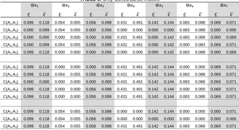
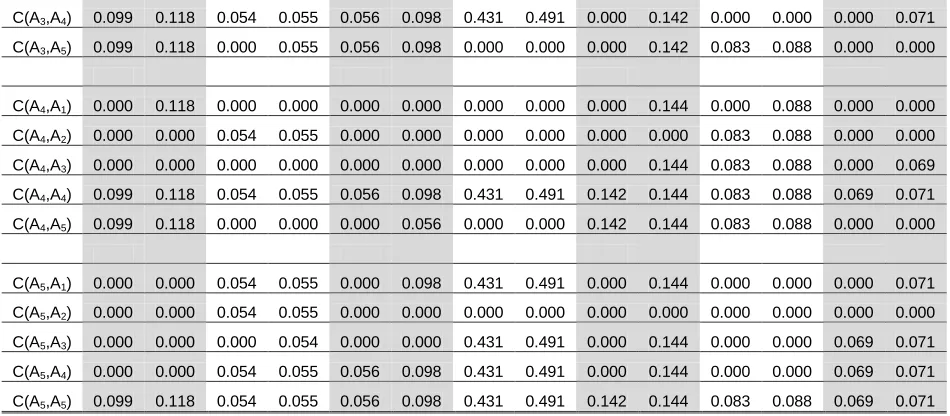
Grey Subjective (Sj) 0.228 0.228 0.020 0.020 0.109 0.109 0.370 0.370 0.156 0.156 0.073 0.073 0.044 0.044 Grey Objective (Oj) 0.036 0.054 0.123 0.127 0.024 0.077 0.440 0.537 0.110 0.114 0.077 0.093 0.093 0.095 Grey Over all (Wj) 0.099 0.118 0.054 0.055 0.056 0.098 0.431 0.491 0.142 0.144 0.083 0.088 0.069 0.071 By applying the procedures of the G-ELECTRE-II method previously discussed in section 3, the grey concordance and grey discordance indices are computed for each pair of alternatives based on Eqs (21-24) as shown in Tables 3 and 5. Then, the grey concordance and grey discordance relations between the alternatives are presented in Tables 4 and 6.
TABLE 3. Grey Concordance Indices
⨂𝒙 ⨂𝒙
⨂𝒙 ⨂𝒙
⨂𝒙 ⨂𝒙
⨂𝒙
0.071 0.069 0.088 0.083 0.144 0.142 0.491 0.431 0.098 0.056 0.055 0.054 0.118 0.099 C(A1,A1)
0.000 0.000 0.088 0.083 0.000 0.000 0.000 0.000 0.056 0.000 0.055 0.054 0.099 0.000 C(A1,A2)
0.069 0.000 0.088 0.083 0.142 0.000 0.491 0.431 0.056 0.000 0.000 0.000 0.000 0.000 C(A1,A3)
0.071 0.069 0.083 0.000 0.142 0.000 0.491 0.431 0.098 0.056 0.055 0.054 0.099 0.000 C(A1,A4)
0.069 0.000 0.088 0.083 0.142 0.000 0.000 0.000 0.056 0.000 0.000 0.000 0.118 0.099 C(A1,A5)
0.071 0.069 0.000 0.000 0.144 0.142 0.491 0.431 0.098 0.000 0.000 0.000 0.118 0.099 C(A2,A1)
0.071 0.069 0.088 0.083 0.144 0.142 0.491 0.431 0.098 0.056 0.055 0.054 0.118 0.099 C(A2,A2)
0.071 0.069 0.088 0.083 0.144 0.142 0.491 0.431 0.000 0.000 0.000 0.000 0.000 0.000 C(A2,A3)
0.071 0.069 0.000 0.000 0.144 0.142 0.491 0.431 0.098 0.056 0.000 0.000 0.118 0.099 C(A2,A4)
0.071 0.069 0.088 0.083 0.144 0.142 0.491 0.431 0.098 0.056 0.000 0.000 0.118 0.099 C(A2,A5)
0.071 0.000 0.000 0.000 0.144 0.142 0.000 0.000 0.098 0.056 0.055 0.054 0.118 0.099 C(A3,A1)
0.000 0.000 0.000 0.000 0.000 0.000 0.000 0.000 0.098 0.056 0.055 0.054 0.118 0.099 C(A3,A2)
0.071 0.000 0.000 0.000 0.142 0.000 0.491 0.431 0.098 0.056 0.055 0.054 0.118 0.099 C(A3,A4)
0.000 0.000 0.088 0.083 0.142 0.000 0.000 0.000 0.098 0.056 0.055 0.000 0.118 0.099 C(A3,A5)
0.000 0.000 0.088 0.000 0.144 0.000 0.000 0.000 0.000 0.000 0.000 0.000 0.118 0.000 C(A4,A1)
0.000 0.000 0.088 0.083 0.000 0.000 0.000 0.000 0.000 0.000 0.055 0.054 0.000 0.000 C(A4,A2)
0.069 0.000 0.088 0.083 0.144 0.000 0.000 0.000 0.000 0.000 0.000 0.000 0.000 0.000 C(A4,A3)
0.071 0.069 0.088 0.083 0.144 0.142 0.491 0.431 0.098 0.056 0.055 0.054 0.118 0.099 C(A4,A4)
0.000 0.000 0.088 0.083 0.144 0.142 0.000 0.000 0.056 0.000 0.000 0.000 0.118 0.099 C(A4,A5)
0.071 0.000 0.000 0.000 0.144 0.000 0.491 0.431 0.098 0.000 0.055 0.054 0.000 0.000 C(A5,A1)
0.000 0.000 0.000 0.000 0.000 0.000 0.000 0.000 0.000 0.000 0.055 0.054 0.000 0.000 C(A5,A2)
0.071 0.069 0.000 0.000 0.144 0.000 0.491 0.431 0.000 0.000 0.054 0.000 0.000 0.000 C(A5,A3)
0.071 0.069 0.000 0.000 0.144 0.000 0.491 0.431 0.098 0.056 0.055 0.054 0.000 0.000 C(A5,A4)
0.071 0.069 0.088 0.083 0.144 0.142 0.491 0.431 0.098 0.056 0.055 0.054 0.118 0.099 C(A5,A5)
TABLE 4. Grey Concordance relations
A5 A4 A3 A2 A1 Concordance indices 𝐶(𝑎, 𝑏) 𝐶(a, b) 𝐶(𝑎, 𝑏) 𝐶(a, b) 𝐶(𝑎, 𝑏) 𝐶(a, b) 𝐶(𝑎, 𝑏) 𝐶(a, b) 𝐶(𝑎, 𝑏) 𝐶(a, b) 0.417 0.238 0.856 0.794 0.730 0.630 0.294 0.142 1 1 A1 0.946 0.945 0.862 0.858 0.789 0.730 1 1 0.858 0.806 A2 0.446 0.294 0.843 0.773 1 1 0.270 0.211 0.426 0.412 A3 0.383 0.348 1 1 0.227 0.157 0.142 0.138 0.206 0.144 A4 1 1 0.818 0.652 0.706 0.554 0.055 0.054 0.762 0.583 A5
TABLE 5. Grey Discordance Indices
⨂𝒙 ⨂𝒙 ⨂𝒙 ⨂𝒙 ⨂𝒙 ⨂𝒙 ⨂𝒙 0 0 0 0 0 0 0 0 0 0 0 0 0 0
D(A1,A1)
9 6 -3 -5 12 11 19 12 4 -1 -5 -10 2 0 D(A1,A2)
1 -4 -6 -8 2 0 -5 -10 6 0 7 5 6 2
D(A1,A3)
-3 -4 1 -2 4 -2 -45 -45 -2 -5 -3 -5 1 -1 D(A1,A4)
4 -2 -8 -11 4 -6 8 4 3 -2 7 5 -2 -2
D(A1,A5)
-6 -9 5 3 -11 -12 -12 -19 1 -4 10 5 0 -2 D(A2,A1)
0 0 0 0 0 0 0 0 0 0 0 0 0 0
D(A2,A2)
-5 -13 -3 -3 -10 -11 -22 -24 2 1 15 12 4 2
D(A2,A3)
-10 -12 6 1 -8 -13 -57 -64 -1 -9 5 2 -1 -1
D(A2,A4)
-2 -11 -5 -6 -8 -17 -8 -11 -1 -1 17 10 -2 -4
D(A2,A5)
4 -1 8 6 0 -2 10 5 0 -6 -5 -7 -2 -6
D(A3,A1)
13 5 3 3 11 10 24 22 -1 -2 -12 -15 -2 -4
D(A3,A2)
0 0 0 0 0 0 0 0 0 0 0 0 0 0
D(A3,A3)
1 -5 9 4 2 -2 -35 -40 -2 -11 -10 -10 -3 -5
D(A3,A4)
3 2 -2 -3 2 -6 14 13 -2 -3 2 -2 -4 -8 D(A3,A5)
12 10
-1 -6 13 8
64 57
9 1 -2 -5
1 1
D(A4,A2)
5 -1
-4 -9 2
-2 40
35 11
2 10 10
5 3
D(A4,A3)
0 0
0 0 0 0
0 0
0 0 0 0
0 0
D(A4,A4)
8 1
-6 -12 0
-4 53
49 8
0 12 8
-1 -3
D(A4,A5)
2 -4
11 8
6 -4
-4 -8
2 -3
-5 -7
2 2
D(A5,A1)
11 2
6 5
17 8
11 8
1 1
-10 -17
4 2
D(A5,A2)
-2 -3
3 2
6 -2
-13 -14
3 2
2 -2
8 4
D(A5,A3)
-1 -8
12 6
4 0
-49 -53
0 -8
-8 -12
3 1
D(A5,A4)
0 0
0 0
0 0
0 0
0 0
0 0
0 0
D(A5,A5)
TABLE 6. Grey Discordance Relations
A5
A4
A3
A2
A1
Discordance indices
𝐷(𝑎, 𝑏) 𝐷(a, b)
𝐷(𝑎, 𝑏) 𝐷(a, b)
𝐷(𝑎, 𝑏) 𝐷(a, b)
𝐷(𝑎, 𝑏) 𝐷(a, b)
𝐷(𝑎, 𝑏) 𝐷(a, b)
0.125 0.088
0.070 0.016
0.123 0.094
0.297 0.211
0.000 0.000
A1
0.266 0.175
0.094 0.035
0.234 0.211
0.000 0.000
0.156 0.088
A2
0.246 0.203
0.141 0.070
0.000 0.000
0.386 0.375
0.175 0.125
A3
0.860 0.828
0.000 0.000
0.625 0.614
1.000 1.000
0.789 0.703
A4
0.000 0.000
0.188 0.105
0.125 0.070
0.266 0.140
0.172 0.140
A5
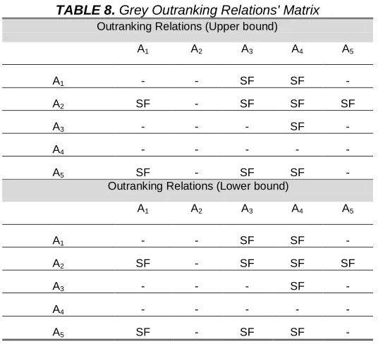
The grey two pairs of threshold values: (C*,D*) and (C−,D−) are shown below in Table 7.
TABLE 7. Threshold Values
D -D*
C -C*
0.15 0.4
0.3 0.5
According to these two pairs of thresholds and the rules mentioned before step 4 of the proposed approach, the grey outranking relations' matrix is shown in Table 8.
TABLE 8. Grey Outranking Relations' Matrix
Outranking Relations (Upper bound)
A5
A4
A3
A2
A1
- SF SF
- -
A1
SF SF
SF -
SF A2
- SF -
- -
A3
- -
- -
- A4
- SF SF
- SF
A5
Outranking Relations (Lower bound)
A5
A4
A3
A2
A1
- SF SF
- -
A1
SF SF
SF -
SF A2
- SF -
- -
A3
- -
- -
- A4
- SF SF
- SF
A5
In the above notation SF stands for the strong outranking relation. For example, A1 SF A4 means that alternative A1 strongly outranks alternative A4. The final ranking of alternatives obtained is A2 A5 A1 A3 A4 for both upper and lowers bounds. As shown it is the same ranking so no need to apply regime method. In case they are different we will apply the regime method.
5.
CONCLUSION
This paper introduces a new grey MCDM based on ELECTRE-II method. The new approach is firstly employing the separation method in a novel way in the area of grey MCDM. A new grey weights' allocation scheme is presented in this work providing grey weights in a new manner. The new grey weights allocation method is combining grey subjective and grey objective weights to conform over all grey weights; this combination is done based on geometric mean in a new way. An illustrative example is given to show the results for testing the proposed approach. Hence, the proposed approach so-called G-ELECTRE-II is practical, realistic, comprehensive and applicable for any grey numbers MCDM problems and very simple to understand and easy to be implemented.
REFERENCES
[1] Belton, V. and Stewart T.J. (2001), Multiple Criteria Decision Analysis: An Integrated Approach, Boston, MA, USA: Kluwer Academic Publishers. [2] Chalekaee, A., Turskis, Z., Khanzadi, M., Amiri, G.
[3] Chakraborty, R., Ray, A and Dan, P. (2013), "Multi criteria decision making methods for location selection of distribution centers", International Journal of Industrial Engineering Computations , 4(4), pp. 491-504.
[4] Datta, S., Sahu, N. and Mahapatra, S. (2013), ―Robot
Selection based on Grey MULTIMOORA
Approach‖, Grey Systems: Theory and
Application, 3 (2), pp. 201-232.
[5] Deng, J. (1982), ―Control Problems and Grey Systems‖, Systems and Control Letters, 5(2), pp. 288-294.
[6] Ezbakhe, F. and Pérez-Foguet, A. (2018), "Multi-Criteria Decision Analysis Under Uncertainty: Two Approaches to Incorporating Data Uncertainty into Water, Sanitation and Hygiene Planning", Water Resources Management, (32), pp. 5169–5182. [7] El-Santawy, M. F. (2012), "A VIKOR Method for
Solving Personnel Training Selection Problem", International Journal of Computing Science, ResearchPub, 1(2), pp. 9–12.
[8] El-Santawy, M. F. and Ahmed, A. N. (2012), A VIKOR Approach for Project Selection Problem, LIFE SCIENCE JOURNAL-ACTA ZHENGZHOU UNIVERSITY OVERSEAS EDITION, 9(4): 5878-5880.
[9] Hobbs BF, Meier P. (2000), Energy decisions and the environment: a guide to the use of multicriteria
methods, Boston, MA, USA: Kluwer
AcademicPublishers.
[10] Hokkanen J and Salminen P. (1997),"Choosing a solid waste management system using multi criteria decision analysis", European Journal of Operational Research; 98:19–36.
[11] Kumar,S.(2012), ―Development OF Decision Support Systems Towards Supply Chain Performance Appraisement‖, M.Sc.Thesis, Department of Mechanical Engineering, National Institute of Technology, Rourkela-769008, Odisha, INDIA. [12] Pandian, P. and Natarajan, G. (2010), ―A New
Method for Finding an Optimal Solution of Fully Interval Integer Transportation Problems‖, Applied Mathematical Sciences, 4(37), pp. 1819 - 1830. [13] Roberts, R. and Goodwin, P. (2002), "Weight
Approximations in Multi-attribute Decision Models", JOURNAL OF MULTI-CRITERIA DECISION, 11: 291–303.
[14] Rogers MG, Bruen M, and Maystre L-Y.(1999), Chapter 3: the electre methodology. Electre and decision support. Boston, MA, USA: Kluwer Academic Publishers.
[15] Roy B, and Bertier P. (1972), "La methode ELECTRE II: Une methode au media-planning", In: Ross M, editor, Operational research 1972, North-Holland: Amsterdam; pp. 291–302.
[16] Roy B, and Bertier P. (1971), "La methode ELECTRE II: Une methode de classement en presence de critteres multiples", SEMA (Metra International), Direction Scientifique, Note de Travail No. 142, Paris, 25p.
[17] Roy B. (1968), "Classement et choix en presence de points de vue multiples: La methode ELECTRE", R.I.R.O; 8:57–75.
[18] Shimray, B. (2017), "A survey of Multi-Criteria Decision Making Technique used in Renewable Energy Planning", International Journal of Computer, (25), pp. 124-140.
[19] Triantaphyllou, E., Shu, B., Sanchez, S. N. and Ray, T. (1998), "Multi-Criteria Decision Making: An Operations Research Approach", Encyclopedia of Electrical and Electronics Engineering, (15), pp. 175–186.
[20] Zardari, N. H., Ahmed, K., Shirazi, S. and Yusop, Z. (2015), Weighting Methods and their Effects on Multi-Criteria Decision Making Model Outcomes in Water Resources Management, Springer.