A MODIFIED SIMPLE METHOD TO GENERATE ARTIFICIAL TIME
HISTORIES FROM GIVEN RESPONSE SPECTRUM
Gangsig Shin1
1
Senior Researcher, Division of Operating Reactor Regulation, Korea Institute of Nuclear Safety, Daejeon, Korea ([email protected])
ABSTRACT
Qualification by analysis and qualification by test are widely used for seismic qualification of seismic categorized equipment in nuclear power plants. To use qualification by test method and to use direct integration method as a means of qualification by analysis, time histories of the seismic input to the shake table and to the analysis model are needed. However, using real earthquake data for the seismic time history input is not adequate due to various reasons. Instead, artificial time histories generated from given response spectrum are practically used.
Although there are many methods to generate artificial time histories from given response spectrum, most of them are too complex to understand fully and to modify. In some cases, different sets of parameters shall be determined by trial and error based method, which may takes too much time and effort. In this study, a simple method to generate a time history compatible with a given response spectrum is shown, followed by modified methods to enhance the compatibility and to have artificial time histories with better satisfying new version of NUREG-0800.
INTRODUCTION
Structural integrity and functional capability of nuclear power plant equipment are becoming more and more important since the great earthquake of east Japan. Among various methods for seismic qualification, seismic test and direct integration analysis method needs seismic time history as an input. But, in many cases, it is hard to get real earthquake time history sets and there is no assure that the real earthquake time history sets; if any; can envelop the earthquake which is expected to happen. Thus, sets of artificial time histories derived from response spectrum are commonly used as earthquake inputs to seismic test or analysis.
Response spectrum is series of maximum time responses of one degree of freedom systems with series of natural frequencies due to given earthquake input. Equations of response spectrum can be expressed as below; (Here, let x&&(t) be ground acceleration time history and
t e t h n t j d
n n z w
w
w , )=- 1 -w sin 1- 2
( be 1-dof system with natural frequency wn)
max 0 ) ( max 0 max ) ( sin ) ( 1 ) , ( ) ( ) , ( * ) ( ) ( t t w w t t w w w t
w t d
e t x d t h t x t h t x S t d t j d t n n n d
ò
ò
-= -= = -& & & & & &while, wd z wn
2
1 -=
From equation (1), one can get the response spectrum simply by plotting maximum response value Sd as a function of wn on the
w
´Sd plane. So, response spectrum can be generated using the information about both input (x&&(t)) and the 1-dof system (h(t)) at the same time, while simple Fourier spectrum is nothing but the frequency domain demonstration. And response spectrum varies for different damping, while simple Fourier spectrum has no relation with damping.As one can see from equation (1), getting response spectrum from time history is straight forward. However, getting a time history from given response spectrum is quite tricky, because, in the process of response spectrum generation, the information on x&&(t) and h(t) is supposed to be lost except for the maximum values of time response. Moreover, there can be infinite numbers of x&&(t) matching given response spectrum, due to infinite phase angle set.
PREVIOUS STUDIES ON ARTIFICIAL TIME HISTORY
As discussed above, getting a time history from a given response spectrum is quite tricky and the time history cannot be unique. So, there are plenty of ways to get time histories from a given response spectrum. G. Kost used the ratio between (given) design response spectrum and computed response spectrum to get the time history, and Jun proposed an updated method to G. Kost by bypassing the trial time history generation step. Tsai and P.C. Rizzo researched the method to get more smooth computed response spectrum, by using local suppressing and raising technique. Unlike above methods which are deterministic, E.H. Vanmarcke developed a random vibration method using spectral density function. Later, a modified method of Tsai and P.C. Rizzo method has been proposed by G.S.Shin, the author of this paper. In this paper, compatibility check to guidance of NUREG-0800 revision 3 has been conducted including corrections from previous paper.
TIME HISTORY GENERATION FROM A GIVEN RESPONSE SPECTRUM
Regulatory guidance
There are many response spectra which can be used as a reference (design) response spectrum. In many cases, a design response spectrum is given by design specification. Especially, for nuclear power plant seismic design, ground response spectra recommended by US Nuclear Regulatory Commission are used in most cases for reference seismic ground input. The ground response spectra are mentioned in Regulatory Guide 1.60. Horizontal design response spectra scaled to 1g horizontal ground acceleration presented in Regulatory Guide 1.60 is shown in Figure 1. In this paper, the ground response spectrum with z =5% is used as the reference response spectrum.
In case of artificial time history, regulatory guidance from Revision 3 of NUREG-0800 Section 3.7.1 are as below;
1) The artificial time history should have peak acceleration identical to the peak ground acceleration of the site
2) The strong motion duration is defined as the time required for the Arias Intensity to rise from 5% to 75%
0.010 seconds) and a total duration of at least 20 seconds.
5) Spectral acceleration at 5% damping shall be computed at a minimum of 100 points per frequency decade, uniformly spaced over the log frequency scale from 0.1 Hz to 50 Hz or the Nyquist frequency. The comparison of the response spectrum obtained from the artificial ground motion time history with the target response spectrum shall be made at each frequency computed in the frequency range of interest.
6) The computed 5% damped response spectrum of the accelerogram shall not fall more than 10% below the target response spectrum at any one frequency. To prevent response spectra in large frequency windows from falling below the target response spectrum, the response spectra within a frequency window of no larger than ±10% centered on the frequency shall be allowed to fall below the target response spectrum. This corresponds to response spectra at no more than 9 adjacent frequency points defined in (b) above from falling below the target response spectrum.
7) In lieu of the power spectrum density requirement of Approach 1, the computed 5% damped response spectrum of the artificial ground motion time history shall not exceed the target response spectrum at any frequency by more than 30% (a factor of 1.3) in the frequency range of interest.
In this paper, to avoid PSD calculation, the new guidance from Revision 3 of NUREG-0800 section 3.7.1 ‘SRP Acceptance criteria 1.B\Option 1\Approach 2 is used.
Figure 1. Ground response spectrum given by Regulatory Guide 1.60
Initial Time History
An acceleration time history x&&(t)can be represented as a sum of sinusoids with Nnumber of magnitude An at frequency wn having phase angle fn;
å
=
+ =
N
n
n n
n t
A t
x
1
) cos(
)
( w f
&
As an initial time history, the response spectrum acceleration at wn of the reference response spectrum is used as magnitude An of x&&(t). Phase angle fn(0~2
p
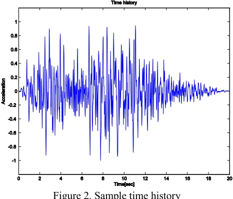
) can be chosen randomly.In this paper, peak ground acceleration is assumed to be unity, so the maximum of the artificial time history is fit to ‘1’ which satisfies the first condition on the artificial time history as mentioned previous section of this paper. To make more realistic characteristics of earthquake acceleration, envelop function is applied. The applied envelop function rises from 5% to 75% satisfying the second guidance on artificial time history. Figure 2 shows a sample time history calculated from the equation (2) followed by envelop function application.
Figure 2. Sample time history
Time increment used in the artificial time history is 0.005 seconds and the total duration is 20 seconds. So this satisfies the fourth condition on the artificial time history. Spectral acceleration at 5% damping along the frequency range of 0.05Hz to 50Hz is considered satisfying the fifth condition on the artificial time history.
Now, 4 conditions(condition 1, 2, 4 and 5) out of 7 are met. 3 remaining conditions will be satisfied at the end of this paper after comparison with the target response spectrum(in this case, ground response spectrum from Regulatory Guide 1.60).
Response Spectrum Matching
Using the initial time history, one can get calculated response spectrum by using equation (1). Here, let the ratio between reference response spectrum(RRS) and calculated response spectrum(CRS)
) , (wn z
R , then the ratio can be represented as
) , (
) , ( )
, (
z w
z w z
w
n n n
RRS CRS
R = (3)
Then, the magnitude of new time history at k+1 step can be calculated as
) , (
, 1
,
z
wn
k n k
n
R A
Now, with the new magnitude An,k+1, new time history &x&(t)k+1 can be formed by equation (2).
Then, new calculated response spectrum at k+1 step can be acquired which will bring a new response spectrum ratio. At the end of this iterative process, final time history with response spectrum which meets the two conditions above can be generated.
RESPONSE SPECTRUM MODIFICATION
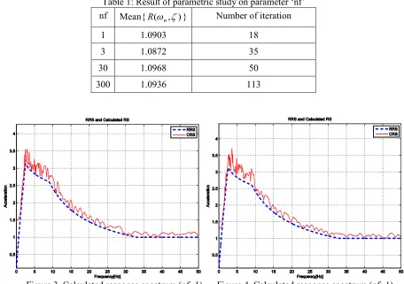
Conventional Method for Response Spectrum Smoothening
An artificial time history was generated in above section. However, as shown in Figure 4, the calculated response spectrum doesn’t match well. Some CRS are too much higher than RRS, some are too much lower. To solve this problem, local response spectrum where CRS exceeds RRS should be suppressed, while CRS below RRS should be raised. In case of simple Fourier spectrum, suppressing and raising can be done simply by lowering and lifting up the corresponding frequency components. On the contrary, we cannot handle the CRS directly. Instead, to modify a response spectrum, input time history should be modified. However, as mentioned in reference by Tsai and Kost, local frequency response spectrum modification cannot be achieved by simply modifying the corresponding frequency component of the input. This is because a response spectrum is generated not only from the input but also from series of 1-dof impulse responses which can weaken the local suppressing and raising effect of input at a certain frequency. To overcome this, Tsai used suppressing and uprising at a single frequency and the adjacent frequency region of that frequency as well. For the region where CRS exceeds RRS, Tsai and Kost used a suppressing method using band stop filter whose amplitude transfer function is
(
)
(
)
(
)
(
)
2 2 2 2 2 2 2 2 2 1 2 1 ú û ù ê ë é W + W + ú û ù ê ë é W W + W -W + W -= F F Hy z z zwhere, W=w wn, z = fraction of critical damping
(5)
For the region where CRS is lower than RRS, a raising method using 1-dof system impulse responses is suggested by Tsai and Kost. These band stop filter method and 1-dof system impulse response method is quite effective. However, as Tsai pointed out at the reference, suppressing method using band stop filter by equation (5) is not straight forward. To get the desired spectrum by using band stop filter method, trial and error approach with different parameters F and z is essential. So it needs time and energy consuming iteration which is not a simple task to find adequate parameters F and z at the same time to get desired response spectrum.
Modified Method for Response Spectrum Smoothening
suppressing/upising the frequency component and the frequency components vicinity of that frequency at the same time. However, at that paper, Shin failed to meet the 4th and 6th condition on the artificial time history. To overcome this, in this paper, the same suppressing/uprising factor for ‘nf’ more frequency components to right and left side of the concerning frequency(2*nf+1 points in total) was used. As one can think, this method is easy and straight forward. Moreover this paper expanded the frequency range from 33Hz to 50Hz to meet the 4th condition and raised minimum range of R(wn,z) from ‘0.9’ to ‘1’ which is relative to the target response spectrum.
RESULTS
Alike other artificial time history generation method, this method uses a suppressing/uprising parameter ‘nf’. Thus, parametric study on this ‘nf’ has been conducted. Table 1 and Figures 3~10 show the result. As shown in Table 1, average ratio between the calculated response spectrum and target response spectrum is slightly higher than ‘1’, satisfying the 3rd condition on artificial time history. And as shown in the table and figures, at any case of suppressing/uprising parameter ‘nf’ will result in the response spectrum ratio R(wn,z)fall within the range between 1 and 1.3 which satisfies the 6
th and 7th condition on artificial time history(when the frequency is greater than 1Hz). And number of iteration until it falls into the range get bigger when ‘nf’ becomes bigger. This seems to be due to lack of fineness which cannot cope with narrow band valleys and peaks in low frequency region.
Table 1: Result of parametric study on parameter ‘nf’ nf Mean{R(wn,z)} Number of iteration
1 1.0903 18
3 1.0872 35
30 1.0968 50
300 1.0936 113
Figure 5. Calculated response spectrum (nf=30) Figure6. Calculated response spectrum (nf=300)
Figure 7. Response spectrum ratio (nf=1) Figure8. Response spectrum ratio (nf=3)
One more thing is about the time history itself. As shown in figures 11~14, time history itself meets the guidance on maximum acceleration and strong motion duration.
Thus, it can be concluded that the artificial time history generated by using this simple method meets all the guidance in the new version of NUREG-0800 section 3.7.1.
Figure 11. Resultant time history (nf=1) Figure12. Resultant time history (nf=3)
Figure 13. Resultant time history (nf=30) Figure14. Resultant time history (nf=300)
FURTHER STUDY TOPIC
One thing to be further studied is that the low frequency (below 1Hz) response spectrum ratio is more than 1.3, which does not comply with the 7th condition on the artificial time history. This seems to be due to low frequency range distortion during Fourier transformation and invert Fourier transformation. At this moment, this is just an engineering guess, so further study shall be conducted to find out the root-cause of this low frequency mismatch.
CONCLUSION
A modified simple method to generate artificial time histories is suggested in this study. Throughout this study, it is proven that the modified method can generate artificial time histories with better compatibility with given response spectrum. At the same time, the modified simple method satisfies new version of NUREG-0800 in the frequency region of 1Hz to 50Hz. However, the low frequency(less than 1Hz) mismatch needs to be further studied.
REFERENCES
G. Kost, T.Tellkamp, H.Kamil, A.Gantayat and F.Weber. (1978). “Automated generation of spectrum-compatible artificial time histories,” Nuclear Engineering and Design, 45, 243-249.
G.S. Shin, J.S. Kim and S.M. Lee. (2008). A Simple and Modified Method to Generate Time History Data from Given Reference Response Spectrum, Inter-noise, Shanghai, China.
Nien-Chien Tsai (1972), “Spectrum-compatible motions for design purpose,” Proc., American Society of civil Engineering, 345-356.
P.C Rizzo, D.E. Shaw and S.J Jarecki. (1975). “Development of real/synthetic time histories to match smooth design spectra,” Nuclear Engineering and Design, 32, 148-155.
US Nuclear Regulatory Commission (1973). Regulatory Guide 1.60 Design Response Spectra for Seismic Design of Nuclear Power Plants. Washington, USA.