Abstract
TOMPKINS, MICHAEL JOHN. Automated Method for Fiber Length Measurement. (Under the direction of Jon Paul Rust.)
The price of cotton is dictated by quality and the most significant factor
contributing to the fiber quality is the length distribution of the fibers contained within the population. Therefore it is of importance to accurately and repeatably measure the length of fibers within a population so that it is graded properly. Current methods are inadequate and thus prior work focused on designing a machine to directly measure individual cotton fibers using digital imaging. The current work begins with the evaluation of the effectiveness of the digital imaging machine. The machine was
evaluated and sources of error identified. Modifications were implemented in an attempt to improve the error. After multiple modifications with little success an entirely new design was conceptualized. The new design aimed to eliminate all major sources of error with the existing machine while not creating new sources of error. The new design is discussed and the results are compared to those obtained by the original imaging
AUTOMATED METHOD FOR FIBER LENGTH MEASUREMENT
by
MICHAEL JOHN TOMPKINS
A thesis submitted to the Graduate Faculty of North Carolina State University
in partial fulfillment of the requirements for the degree of
Master of Science
TEXTILE ENGINEERING
MECHANICAL ENGINEERING
Raleigh 2006
APPROVED BY:
_____________________________ _____________________________ Dr. Jeffrey Joines Dr. Gregory Buckner
Biography
Michael J. Tompkins was born in Pittsburgh, Pennsylvania on March 2nd 1982 to Dennis and Paula Tompkins. He spent most of his childhood in Charlotte, NC where he lived with his parents and two brothers Johnathan and Zachary Tompkins. He played soccer through elementary, middle, and high school while also being active in the Boy Scouts where he attained the rank of Eagle Scout. In 2000 he enrolled in the Textile Engineering program at North Carolina State University. He remained active in sports playing club Rugby for much of his collegiate career. He graduated Cum Laude in 2004 with a degree in Textile Engineering. He immediately enrolled in the Masters program pursuing a co-major in Textile and Mechanical Engineering. He currently enjoys driving and
Acknowledgements
I would like to thank Dr. Jon Rust for giving me the opportunity to work on such an interesting project, and for his guidance, patience, and trust throughout the process. I would like to thank the College of Textiles and North Carolina State University for providing me with the financial support required to complete the project.
Table of Contents
Page
List of Figures ...vii
List of Tables ...ix
1.0 Introduction...1
2.0 Technology Review...3
2.1 Fiber Length Measurement ...3
2.2 Camera ...3
2.2.1 Charge Coupled Device (CCD) ...4
2.2.2 Complimentary Metal Oxide Semiconductor (CMOS) ...5
2.2.3 CCD vs. CMOS ...6
2.3 Light Sensing...8
2.3.1 Photodiode...8
2.3.2 Phototransistor ...9
2.3.3 Photoresistor ...10
2.4 Illumination ...10
2.4.1 Light Emitting Diode ...10
2.4.2 Xenon Strobe ...12
2.5 Conclusion...13
3.0 Previous Image Based Fiber Length Measurement System ...14
3.1 Description of Original Design ...14
3.2 Investigation of Possible Causes of Error...18
3.3 Analysis of Error ...21
3.4 Research Objectives...22
4.0 Design Solutions to Eliminate Error...23
4.1 Design Solution Using Current Device Technology ...23
4.1.1 Backlighting Using Transparent Belt...23
4.1.1.1 Components and Operation ...24
4.1.1.2 Preliminary Tests ...26
4.1.1.3 Evaluation of System Feasibility ...26
4.1.2 Frontlighting Using Opaque Belt...27
4.1.2.1 Overview of Components and Operation ...29
4.1.2.2 Preliminary Testing ...31
4.1.2.3 Evaluation of System Feasibility ...32
4.2 Control Without Contact...34
4.2.1 Control Without Contact Using Electrostatic Plates...35
4.2.1.1 Proposed Methodology...35
4.2.1.2 Analysis of Feasibility...36
4.2.2 Control Without Contact: Air Stream ...37
4.2.2.1 Proposed Methodology...38
4.2.2.2 Analysis of Feasibility...40
5.0 Final Design ...42
5.1.2 Final Design...46
5.1.3 Analysis of Effectiveness ...51
5.2 Fiber Transport Enclosure...52
5.2.1 Method ...52
5.2.1.1 Air Gap ...52
5.2.1.2 Coanda Effect...54
5.2.2 Enclosed Transport System ...54
5.2.2.1 Preliminary Enclosed Fiber Design ...55
5.2.2.2 Preliminary Design Problems ...56
5.2.2.3 Redesigned Fiber Transport Enclosure ...57
5.2.2.4 Redesigned Fiber Transport Enclosure Design Problems ...58
5.2.2.5 Redesigned Fiber Transport Enclosure ...58
5.2.2.6 Redesigned Fiber Transport Enclosure Design Problems ...59
5.2.2.7 Analysis of Design Solutions...59
5.2.3 Final Design...60
5.2.3.1 Theory...60
5.2.3.2 Material Selection ...66
5.2.3.3 Final Design Evaluation ...67
5.3 Light Source ...68
5.3.1 Method ...68
5.3.2 Existing LED Backlight ...69
5.3.3 Ultra bright Led Array...70
5.3.3.1 Theory...70
5.3.3.2 Ultra bright Led Array Feasibility...73
5.3.3.3 Analysis ...75
5.3.4 Xenon Strobe ...78
5.3.4.1 Theory...78
5.3.4.2 Xenon Strobe Feasibility ...80
5.3.4.3 Analysis ...81
6.0 Camera...82
6.1 Required Features ...82
6.2 Camera Integration ...84
6.3 Conclusion...85
7.0 Software...86
7.1 Existing Software ...86
7.2 New Fiber Analysis Software ...88
7.2.1 Image Capture Software...88
7.2.2 Image Processing ...89
7.2.2.1 Thresholding ...89
7.2.2.2 Filling ...94
7.2.2.3 Remove Noise...96
7.2.2.4 Thinning...97
7.2.2.5 Calculating Fiber Length...99
7.3 Visual Interface ...101
7.3.2.1 Database Design...102
7.3.2.2 Visual Interface ...105
7.3.2.3 Conclusion ...113
8.0 Current State of Technology... 114
8.1 Overview of System ...114
8.2 Testing...116
8.2.1 Fiber Position Test ...116
8.2.3 Analysis of Results...117
8.2.3 Sources of Error...119
8.2.4 Solutions to Error...120
8.3.1 Evaluation of Measurement Accuracy and Repeatability ...121
8.3.2 Analysis of Results...122
8.3.4 Sources of Error...126
8.3 Evaluation of System Improvement ...128
9.0 Conclusion ... 131
List of Figures
Page
Figure 2.1 CCD Chip Diagram (Reproduced From [20]) ...5
Figure 2.2 CMOS Chip Diagram (Reproduced From [20]) ...6
Figure 3.1 System Diagram ...16
Figure 3.2 Sample Image...17
Figure 3.3 Rayon Mix...19
Figure 3.4 Best Run...20
Figure 3.5 Typical Run...20
Figure 3.6 Overlap Diagram ...21
Figure 4.1 Transparent Belt Diagram...24
Figure 4.2 Transparent Belt System...25
Figure 4.3 Transparent Belt Image...25
Figure 4.4 Opaque Belt Diagram ...28
Figure 4.5 Opaque Belt System ...28
Figure 4.6 Rotating Belt System...30
Figure 4.7 Rotating Belt Close Up ...31
Figure 4.8 Opaque Belt Image ...32
Figure 4.9 Rotating Belt Image...33
Figure 4.10 Broken Skeleton Closeup...34
Figure 4.11 New System Concept...40
Figure 5.1 IR Emitter / Detector Diagram...43
Figure 5.2 Laser / Photodiode Diagram ...44
Figure 5.3 Reflected Laser / Photodiode Diagram...45
Figure 5.4 Photodiode Spectral Response [22]...46
Figure 5.5 Photodiode Amplifier Circuit [21] ...47
Figure 5.6 Difference Amplifier [5]...48
Equation 5.1 Difference Amplifier Equation [5] ...49
Figure 5.7 Sensor Circuit Diagram ...50
Figure 5.8 Camera Trigger Circuit [25] ...51
Figure 5.9 Air Gap System ...53
Figure 5.10 Preliminary Enclosed Design...55
Figure 5.11 Redesigned Enclosure...56
Figure 5.12 Viewing Area Contour...57
Figure 5.13 Tapered Contour...59
Figure 5.14 Final Enclosure Contour ...61
Figure 5.15 Enclosure Design...62
Figure 5.16 Sandwich Design ...63
Figure 5.17 Wireframe Sandwich Design ...63
Figure 5.18 Exploded View ...64
Figure 5.19 Entrance Adapter Top...65
Figure 5.20 Entrance Adapter Bottom ...65
Figure 5.23 LED Driver Circuit [1] ...72
Figure 5.24 LED Array Design...73
Figure 5.25 Xenon Strobe Circuit Diagram...80
Figure 6.1 Resolution Example...82
Figure 6.2 Resolution Example...82
Figure 6.3 Camera Trigger Diagram [25]...84
Figure 6.4 Camera GPO Diagram [25]...85
Figure 7.1 FFT Graph...91
Figure 7.2 Original Image...92
Figure 7.3 Image Post FFT ...92
Figure 7.4 Thresholded FFT Image...92
Figure 7.5 Thresholded FFT Image...92
Figure 7.6 Thresholded Image ...95
Figure 7.7 Filled Image ...96
Figure 7.8 Cleaned Image...97
Figure 7.9 Post Thinning Image...98
Figure 7.10 Thinned Fiber ...98
Figure 7.11 Cleaned Image...98
Figure 7.12 Cleaned Close up...98
Figure 7.13 Find Length ...100
Figure 7.14 Find Length Close Up...100
Figure 7.15 Database Design ...103
Figure 7.16 Menu ...106
Figure 7.17 View History ...107
Figure 7.18 Camera Settings... 108
Figure 7.19 Calibrate Camera ...109
Figure 7.20 Calibrate Resolution ...110
Figure 7.21 Calibrate Camera ...111
Figure 7.22 Calibrate Resolution ...112
Figure 8.1 Fiber Position Data ...Error! Bookmark not defined. Figure 8.2 Fiber Position Test – Cleaned Data ...118
Figure 8.3 Fiber Length Graph ...123
List of Tables
Page
Table 5.1 Fiber Speed Calculations...76
Table 8.1 Fiber Position Test ...117
Table 8.2 Fiber Position Test Statistics – Cleaned Data ...118
Table 8.3 Fiber Position Test ANOVA Results – Cleaned Data ...119
Table 8.4 Average Accuracy Statistics...123
Table 8.5 Individual Accuracy Statistics...123
Table 8.6 Average Accuracy Statistics – Broken Skeletons Removed...124
Table 8.7 Individual Accuracy Statistics – Broken Skeletons Removed ...124
Table 8.8 Fiber Length ANOVA Results ...125
Table 8.9 Fiber Length ANOVA Results – Broken Skeletons Removed ...126
Table 8.10 System Comparison ...128
1.0 Introduction
Previous work in the area of novel cotton fiber length measurement instrumentation at the college of textiles involved designing a machine that could continuously deliver individual fibers to a viewing area at which point they were analyzed and their length determined. Subsequent work improved the system in a number of areas including comparing the accuracy of the machine to known fiber length measurement machines. The goal of this following work is to further improve the systems ability to accurately and repeatably measure the length of cotton fibers.
In order to improve the system, errors in the existing system were characterized and their sources determined. Upon identifying the primary sources of error,
modifications to the system were conceptualized, implemented and tested. The modifications consistently did not provide the desired improvement and it quickly became apparent that a new system was required.
The new system was developed with the intent to control the fibers without any form of physical contact. Five development areas were identified: the sensor, the enclosure, the light source, the camera and finally the software. Each area required individual development culminating in the integration of all components into a complete system.
The enclosure would provide a means to control the fiber as it travels past the sensor and into the viewing area. The enclosure was designed so that it did not obstruct a portion of the fiber from the camera or cause fibers to remain in the enclosure. By
carefully selecting the contour of the enclosure, the path and movement of the fiber could be accurately controlled.
A strobe light was implemented in order to freeze the motion of the fibers as they entered the viewing area. In order to provide the required contrast for image processing the light needed to be very bright, however, it also needed short strobe duration. The fiber is constantly moving and the amount the fiber moves during the time the strobe is on is shown as blur on the image. Blur significantly decreases the ability of the image processing software to accurately analyze the fiber and must be minimized.
A new camera was needed to both control the timing of the sensor, strobe, and image capture while also providing high quality images for capture. The camera selected met all criteria and was able to control the synchronization of all components while providing clear images.
2.0 Technology Review
In order to design an effective machine, a thorough understanding of a variety of different components was needed. To determine what was available and what was most suitable for the future system, each area needed to be thoroughly researched. The first area of research was the camera. Second, a number of different sensing technologies needed to be investigated, including photodiodes and other light detection techniques. Third, lighting sources needed to be evaluated to determine the most suitable for the specific application. With a thorough understanding of existing technology, the design of the system can be optimized by utilizing the best components for the specific application. 2.1 Fiber Length Measurement
The length of cotton fibers is of primary importance when quantifying the quality of a cotton population. Methods currently exist to evaluate the length of cotton fibers however, they are inadequate and are known to have significant error. High Volume Instrumentation (HVI) measures fibers in bulk while the Advanced Fiber Information System (AFIS) measures fibers individually, however, in both cases, the length is measured indirectly [8]. Measuring the length indirectly introduces significant amounts of error into the measurement. Recent work has been completed to directly measure individual fibers and while a step in the right direction, it is not ready to replace the existing methods. For a more complete and detailed explanation of existing fiber length measurement technologies refer to the work of Stroupe and Byrd [29] [8].
2.2 Camera
computer. The secondary purpose of the camera is to provide the control over the light source through the use of output triggering. When selecting a camera, the primary purpose of image capture needs to be at the top of the selection criteria. While still considering image quality, resolution is a concern as it will affect the contrast of features within the image along with the processing time after the image is captured. For machine vision, Charge Coupled Device and Complimentary Metal Oxide Semiconductor are the two primary digital camera technologies that are to be considered.
2.2.1 Charge Coupled Device (CCD)
CCD technology has undergone a great deal of improvement and optimization since its inception in the early seventies, and thus has been the traditional choice when selecting a digital imaging technology [7]. CCD’s consist of a 2D array of
photodetectors (either photodiodes or photogates) arranged in a series of rows and
Figure 2.1 CCD Chip Diagram (Reproduced From [20])
2.2.2 Complimentary Metal Oxide Semiconductor (CMOS)
Figure 2.2 CMOS Chip Diagram (Reproduced From [20])
2.2.3 CCD vs. CMOS
There are eight attributes that determine the overall quality of the chip: Responsivity, Dynamic Range, Uniformity, Shuttering, Speed, Windowing, Anti-Blooming, and Biasing and Clocking. Responsivity refers to the amount of charge created by the photodetector per unit of light reaching the photodetector. In terms of responsivity, CMOS chips are slightly superior due to the ease at which the amplifiers can be placed. A CMOS chip allows low power, high gain amplifiers to be used whereas CCD requires higher power amplifiers [20].
capacitance variations, and transistors which can more easily be configured to minimize noise, all of which contributes to a reduction of noise within the images [20].
The difference in pixel response across the array to the same light intensity is the uniformity of the image sensor. CCD’s are generally more uniform than CMOS image sensors because of the individual amplifiers used to convert each pixel charge into a voltage. Using multiple amplifiers decreases uniformity because the charge of each pixel does not always get amplified uniformly. By implementing amplifiers using feedback, the uniformity is increased, however, it is still slightly inferior to CCD technology [20].
Shuttering is that ability of the camera to stop and start the exposure at prescribed times. CCD technology is superior when it comes to shuttering since implementing shuttering in CMOS requires a number of transistors at each pixel. The transistors take up space around the pixel increasing the physical size of each pixel. A rolling shutter can be used to decrease the number of transistors at each pixel by exposing different lines of pixels at different times, however the use of this technique results in a blurry image when there is a fast moving target [20].
CMOS is faster than CCD due to the ability to place all of the supporting circuitry on the same chip. By placing all circuitry on the same chip the distances between
components, inductance, capacitance, and propagation delays are all decreased.
Windowing refers to the ability to select a region of pixels to view, and ignore all other pixels. CMOS imaging chips allow the user to select a region of interest and only output the selected pixels, while CCD’s are limited in this capability [20].
is inherently superior at draining excess charge from saturated pixels, while CCD’s require specific engineering to achieve the same effect [20].
CMOS also has an advantage in terms of biasing and clocking because they operate at a single bias voltage and clock level. CCD’s often require higher bias
voltages; however newer clocks have been simplified to run on low voltage clocks [20]. 2.3 Light Sensing
There are many methods used to convert light energy into either a voltage or a change in resistance, both of which can easily be used to sense the presence of light. Photodiodes and phototransistors actually convert light energy into a small detectable voltage, while photoresitors change resistance in the presence of light. Both methods provide a means with which to detect the presence of light.
2.3.1 Photodiode
A photodiode is simply a diode in which the p-n region is exposed enabling a current to flow from the n to the p region when exposed to light. Diodes consist of two differently doped regions of semiconducting material, one region is the p region
consisting of holes, and the other region is the n region consisting of electrons. [5] The diode acts as a gate allowing current to flow freely when forward biased, however, if reversed biased, current is not allowed to flow freely. To be forward biased, the positive terminal of the battery must be connected to the p region and the negative terminal to the n region. Current will not flow when forward biased until the applied voltage reaches the contact potential for silicon (.6V-.7V).
photodiode in the forward biased configuration the freed electrons will flow, resulting in a current. The diode can similarly be used in the reverse biased configuration and act as a switch. Diodes have a significant resistance to current flow when reversed biased
however when light is present the resistance is significantly decreased, and current is allowed to flow [12]. It takes a significant amount of light to create appreciable currents when forward biased, however, when reversed biased the photodiode is sensitive to much smaller quantities of light. [5]
2.3.2 Phototransistor
Transistors are similar to diodes in that they contain differently doped regions of a semiconducting material, however, transistors contain three regions and are used to either amplify current or switch current on and off. The applicable types of transistors to
phototransistors are the npn and the pnp types of BJT transistors. Both transistors contain three doped regions, known as the base, collector and emitter. For simplicity’s sake, the npn transistor will be the focus of the discussion, however, a pnp transistor is similar only with a different organization of doped regions. The collector is doped as a “n” region, the base is a “p” region and the emitter is a heavily doped “n” region. By applying current to the base region the current allowed to flow between the collector and emitter regions can be controlled. [5]
2.3.3 Photoresistor
Photoresistors differ from photodiodes and phototransistors in that instead of converting light into a voltage, or using light to switch on a current, they use light to lower their resistance. Photoresistors are made from a high resistance semiconductor able to absorb photons in the presence of light. The photons add energy to the electrons, allowing them to move to the conduction band of the semiconductor. The free electron and resulting hole will conduct electricity and effectively lower the resistance of the semiconducting material. When incorporated in a voltage divider with a resistor the change in resistance can cause a measurable change in voltage. Photoresistors have a very slow rise and decay time limiting their use to low speed applications.
2.4 Illumination
If the camera is the primary focus when designing a machine vision system, the light source would be a very close second. The proper lighting can produce a very crisp useful image, while improper lighting can produce an image that is blurry, too bright, or to dark; rendering the image useless. While there are numerous different lighting sources available, there are fewer possibilities when considering strobing light sources. Light emitting diodes or LED’s are commonly used for strobing applications due to their low cost, long life, and simplicity. Another strobe light technology is the Xenon strobe which is known for its high intensity, short duration flash.
2.4.1 Light Emitting Diode
“n” side the electrons come into contact with holes. As the electrons contact these holes energy is released in the form of a photon and emitted as light. The wavelength of the light is dependent on the bandgap energy of the materials used to create the p-n junction. Normal diodes are made of materials that do not release photons when the holes are filled by electrons and LED’s are made of materials that release photons in a specific
wavelength to produce a desired color [12].
LED’s require low voltages to operate and are therefore much easier to work with and integrate into sensitive electronics. Because they do not draw a lot of power, LED’s are also low temperature, enabling them to be used in a number of applications where temperature would either be a safety concern, or potentially harmful to the surrounding components. LED’s do not have a filament or any moving parts and are therefore quite durable and ideally suited for use in environments with significant vibration or g-forces [12].
LED’s are small and do not produce significant amounts of light by themselves requiring many LED’s to be combined into an array for many machine vision
applications. Not only is an array of LED’s brighter than a single LED, but the array is also more uniform than a single light source. By incorporating an array of LED’s with simultaneous control, an effective backlight can easily be created. LED’s are not very bright when compared to xenon strobes, and while multiple units can easily be combined, there is a limit to how many can be placed in a certain area.
increasing the range of applications. To ensure that the light from the Luxeon LED’s is uniform the current used to drive a series of LED’s needs to be controlled rather than controlling the voltage [21].
2.4.2 Xenon Strobe
Xenon strobes provide a high intensity short duration flash useful for freezing the motion of moving parts. A xenon flash lamp consists of a fused quartz tube filled with xenon gas, along with three electrodes; a positive electrode, a negative electrode, and an electrode used to apply a high voltage to the gas. In a xenon flash lamp, the xenon gas acts as a filament conducting the electricity between the two electrodes. Under normal conditions, the gas does not act as a conductor and the potential difference between the two electrodes is not enough to jump the gap. When a small transformer known as a trigger coil applies a high voltage (~4kV) to the third electrode, the gas becomes ionized and conductive. Current is now allowed to flow between the positive and negative electrode and the rapid discharge results in a flash. Energy is stored prior to discharge in a capacitor, the size of which affects the duration and intensity of the strobe. A smaller capacitor will produce a shorter, less intense flash while a larger capacitor will produce a longer more intense flash [9, 16].
duration. Xenon flashes contain a complete spectrum of wavelengths between 150 nm all the way up to 6µm. To the human eye the light appears to be white but with the use of different types of filters any specific wavelength can be extracted to meet a specific need. 2.5 Conclusion
With a thorough understanding of the different types of components that could be integrated into the system an informed decision could be made for each component. While the specific characteristics of each component are a concern; cost, availability and ease of integration are difficult to assess when comparing general technologies. A thorough search of specific components was conducted for each area to compare specific products instead of technologies in order to select the optimal product for each
3.0 Previous Image Based Fiber Length Measurement System
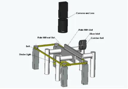
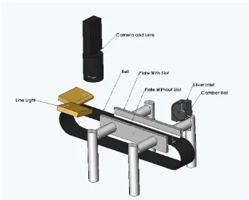
The original machine was designed to individualize cotton fibers, control them, and introduce them into the viewing area where an image could be captured and analyzed. A modified comber roll was used to separate individual fibers from a sliver and introduce them to an electrostatic field. The electrostatic field was created between two aluminum plates designed to draw the fiber towards a urethane belt running through a slot in the center of one of the plates. The fibers would attach themselves to the belt and be transported to the imaging area at which point they would be illuminated by a strobe light and their image would be captured. Image analysis software was then used to determine the lengths of the fibers within the image. While this was an effective system there were some fundamental errors which proved very difficult to overcome.
3.1 Description of Original Design
The original design consisted of four fundamental mechanisms; the fiber
which the fibers were introduced into the system. Controlling the number of fibers introduced to the system allowed the fiber density on the belt and thus the number of fibers per image to be controlled. Having precise control of the density of fibers allowed the number of crossovers to be minimized while ensuring that there were as many
individual fibers in each frame as possible.
The comber roll removed individual fibers from a sliver and introduced them into the electrostatic field created between two plates by a high voltage power supply
backlighting the fibers, the camera sees a silhouette of the fiber which is optimal for software analysis.
The strobe light was a backlight made by CCS (Reference) which consisted of an array of many small LED’s behind a diffuse plate to ensure the light was uniform. The light was driven by a strobe controller which allowed the adjustment of the intensity of the light along with the duration of the strobe pulse from 10 µs to 990µs. The camera used a 1.3 megapixel CCD digital camera made by Pulnix and was connected to the computer using a framegrabber. The camera and strobe light did not need to be
synchronized to effectively capture fibers within the frame. Since there was a high fiber density on the belt the camera and strobe could run continuously and consistently capture images containing fibers.
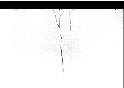
Figure 3.2 Sample Image
the diagonal direction. The length of the fiber is simply the distance calculated by the outline divided by two. The software allowed the number of fibers per sample to be selected and then displayed the length distribution of the sample along with important statistics while saving the data for future analysis.
3.2 Investigation of Possible Causes of Error
Significant effort went into determining the accuracy and precision of the
machine. Because the machine is itself a measurement system it is difficult to determine the accuracy using sliver because the actual lengths of the fibers that were measured are not known. To evaluate the accuracy and precision, experiments were run using different slivers, cut length rayon, and cut length cotton.
The first experiment was designed to determine if the machine could differentiate between two different slivers. An experiment was designed with multiple runs for each sliver and randomized to eliminate error. Two slivers collected from different bales at different times were tested multiple times. The experiment was set up to allow a number of parameters to be tested. Sample size, sliver, and date were all tested to determine the individual effects on the data. The machine was thoroughly cleaned in between each run to ensure fibers from the previous run would not contaminate the sample. This
experiment proved successful with the machine proving its ability to measure a statistical difference between the slivers. However the date also showed a statistical difference showing that there is significant run to run variation caused by the machine.
system that would more favorably select one length as opposed to another. The different lengths of fibers were weighed and thoroughly mixed together so that the ratio of fibers by number was known. The fibers were then fed into the machine by hand since it proved unrealistic to form a sliver out of such short fibers. The ideal result would have been a clear transition once the fiber lengths were sorted from the longer fibers to the shorter fibers.
Rayon M ix
0 0.1 0.2 0.3 0.4 0.5 0.6 0.7
1 13 25 37 49 61 73 85 97 109 121 133 145 157 169 181 193 205 217 229 241 253 265 277 289 301 313 325 337 349 361 373 385 397 409 421 433 445
Fiber Number
Rayon M ix
Figure 3.3 Rayon Mix
The actual result was less than ideal in that the smaller rayon fibers were not noticeable at all. There would have ideally been a significant number of fibers approximately .5 inches which are present in the graph however there would have also been a distinct drop in length to approximately .25 inches. There is a drop, however it is gradual and does not distinctly show that there were .25 inch fibers in the image. This experiment proved that there is a significant bias toward longer fibers.
the software does display a histogram, Excel allows all of the runs to be viewed side by side for comparison.
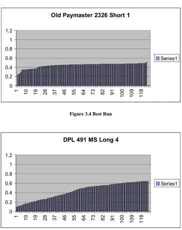
Old Paymaster 2326 Short 1
0 0.2 0.4 0.6 0.8 1 1.2
1 10 19 28 37 46 55 64 73 82 91
100 109 118
Series1
Figure 3.4 Best Run
DPL 491 MS Long 4
0 0.2 0.4 0.6 0.8 1 1.2
1 10 19 28 37 46 55 64 73 82 91
100 109 118
Series1
Figure 3.5 Typical Run
of a fiber. However the second graph containing .65in fibers is indicative of most of the results gained from the experiment and paints a different picture all together. This
sample clearly shows that while it measures a few fibers at the actual length the measured length quickly drops and a majority of the fibers are measured far less than their actual length.
3.3 Analysis of Error
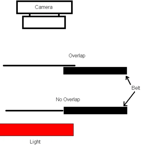
The problem was known but the severity of the problem was not, prior to the test using the cut length fibers. The primary problem is that an unknown portion of the fiber overlaps the belt and therefore cannot be seen by the camera. If the fibers overlapped the belt a consistent amount it would be easy to compensate for that error however, as the graph clearly shows, an amount of fiber that overlaps the belt ranges from none to almost the entire fiber.
Before the cut lengths were used, the error was assumed to be spread out over many possible sources. Breakage caused by the comber roll, selection bias, and broken skeletons were all thought to contribute equal parts to the overall error. Since all the fibers were the same length selection bias is immediately eliminated as a source of error, and while breakage is still a factor it is highly unlikely that every fiber would be broken which is the only way that such a distribution would be created. Broken skeletons are still a possibility however by individually viewing each image the effect was found to be minimal.
3.4 Research Objectives
After characterizing the error in the previous system it became evident that both the accuracy and repeatability of the system needed to be improved. A number of factors were considered when attempting to improve the accuracy and repeatability. The
4.0 Design Solutions to Eliminate Error
The problem with overlap was the focus on all subsequent research. The goal is to control the fibers in a matter that allows the entire fiber to be seen by the camera. The first attempts at solving the problem utilized the same machine and involved modifying the belt to try and ensure the entire fiber would be visible. To test each new design, a prototype was constructed and tested by collecting images without using the software since the software made assumptions unique to the original machine. The images were evaluated subjectively, and by analysis with modified software, simulating analysis with the actual software. Based on this analysis the potential of the system could be evaluated and a decision could be made whether to proceed or redesign.
4.1 Design Solution Using Current Device Technology
The first solutions developed were based on modifying the current technology in an attempt to overcome the specific problem areas. Prototypes were constructed for each concept and tested to determine the overall improvement.
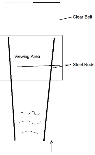
4.1.1 Backlighting Using Transparent Belt
Figure 4.1 Transparent Belt Diagram
4.1.1.1 Components and Operation
A number of belt materials were tested, however, it quickly became evident that the belt would build up static attract the fibers to the belt and not allow them to be easily removed. Since the fiber stuck to the belt due to static and not the electrostatic field, they were not oriented properly and also could not be easily removed with suction.
Figure 4.2 Transparent Belt System
4.1.1.2 Preliminary Tests
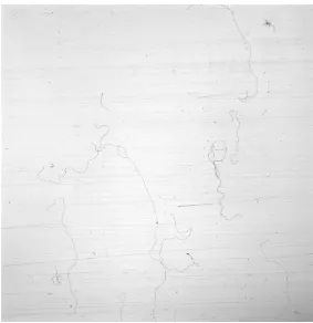
The first test run consisted simply of running the comber roll to populate the belt with fibers and running the camera continuously to evaluate the image quality and the fiber orientation. A sample image is shown in Figure 4.3. The original evaluation showed promise and while the image quality was not perfect, it was good enough to warrant further evaluation. To further test the viability of the new system, the samples captured from the continuously running camera were analyzed using a free standing version of the software. The software was modified slightly so that it would simply threshold the fiber. By only thresholding the fiber it was easy to see the quality of the image from a software analysis standpoint.
4.1.1.3 Evaluation of System Feasibility
would fall. Another issue that became evident when the image was thresholded was the effect of scratches. Scratches on the belt show up in the image and when thresholded, appear as separate fibers or as additions to actual fibers. While it may be possible to select a belt material or drive roller material that reduces scratches, it is unlikely that scratches can be completely eliminated. While the system performed similarly to what was expected, there were serious issues that quickly became obvious. While each
problem in itself may not have been insurmountable the combination of problems yielded a system that was no better than the original design.
4.1.2 Frontlighting Using Opaque Belt
Figure 4.4 Opaque Belt Diagram
4.1.2.1 Overview of Components and Operation
experienced including the tendency for fibers to extend out of the image. It was obvious that a better way to control fibers was required to ensure that the whole fiber would consistently be captured in the image. A solution would combine the original system with the new belt to allow front lighting. The belt would be horizontal at the imaging area and vertical where the fibers are introduced into the electrostatic field. The fibers would enter and jump back and forth between the plates just as they did in the original system and as they were drawn toward the center they would come into contact with the belt at the point where the belt fits into the slot.
Figure 4.7 Rotating Belt Close Up
As the belt moves toward the viewing area it rotates up and the fibers end up laying on the belt perpendicular to the direction of the belt. A section is removed from the end of the slotted plate so that any fiber end that would extend under the slot would not be lost. This design change worked well and allowed the fibers to be controlled and delivered to the viewing area on top of an opaque belt.
4.1.2.2 Preliminary Testing
Preliminary tests began with running the machine and viewing the samples in a continuous video stream. This gave a general idea of how the fibers looked and allowed the camera and lighting settings to be optimized. During the continuous run, individual images were captured for closer visual analysis and thresholding to evaluate the
4.1.2.3 Evaluation of System Feasibility
The first design showed good contrast once the linelights were used instead of the incandescent lights or the ringlight, however, the fibers were scattered throughout the image and showed little orientation.
Figure 4.8 Opaque Belt Image
After implementing the new belt design in which the belt would rotate as it neared the viewing area the orientation increased significantly. Fibers were still out of frame but that was not a concern and by either widening the frame or removing them
Figure 4.9 Rotating Belt Image
the belt has to be bent to fit in the slot and since the belt is in constant motion it is almost impossible to ensure that the belt is constantly flat.
Figure 4.10 Broken Skeleton Closeup
Considering the number and difficulty of the problems associated with the design it was determined unfeasible and would not have been a significant improvement over the existing solution.
4.2 Control Without Contact
significantly reduced. With this knowledge, the future designs would all enable the fibers to be backlit when they are presented in the viewing area. The commonality with all of the previous unsuccessful concepts was the belt, and more generally contact with the fibers. When the fibers are in contact with part of the machine, it is impossible to avoid the point of contact obstructing a portion of the fiber or causing some addition to the fiber (in the form of scratches in the clear and opaque belt examples). With this realization, future designs focused on controlling the fibers in a manner that would deliver them to the viewing area and present them to the camera with no physical contact.
4.2.1 Control Without Contact Using Electrostatic Plates
The first design concept for controlling the fibers without any physical contact involved a more extreme modification of the existing machine. If the fibers could be released from the belt at the instant they were in the field of view and be captured in an image as they moved toward the opposite plate there would be no obstruction and the entire fiber could be caught within the frame. This design would not require many of the components to be redesigned and it incorporated the belt and electrostatic field which was a proven method of controlling fibers.
4.2.1.1 Proposed Methodology
fibers to discharge, causing the fibers to remain stuck to the belt and rarely jump off. The focus of the investigation was to create a situation in which the fibers would jump off the belt predictably when the belt reached the viewing area. The first idea was to find or build a belt which is semi-conductive and would allow the fibers to slowly discharge until they reach some critical charge at which point they would jump toward the opposite plate. Polymers are commonly mixed with carbon to provide some conductivity and eliminate or reduce static buildup. Another proposed solution involved placing a conductor at the viewing are that would contact the fibers as they traveled past on the belt. Upon contacting the belt, the fibers would discharge and jump off the belt into the viewing area.
4.2.1.2 Analysis of Feasibility
of the fibers not being captured at all or being partially in frame. These fibers cannot be analyzed since some unknown portion of the fiber is not visible. Sensing the fibers as they are released was considered but again thought unrealistic because no such sensor was available or practical in such a configuration. Also even if a sensor were available there would not be enough time to sense the fiber and trigger the camera before the fiber would have passed through the viewing area. The second scenario using the conductor to contact the fiber and allow the charge to discharge causing the fiber to release from the belt suffered from many of the same shortcomings as the semi-conductive belt design. In addition, there was a good possibility that since the conductor would be a charge
concentration that fibers would be attracted to this point. This would cause fibers to jump back and forth between the plate and the conductor which would be in the middle of the viewing area. This would likely cause entanglements or erroneous readings from measuring the same fiber multiple times. Overall, while the thought process was in the right direction the concepts developed were theoretically unfeasible and thus more potential solutions were needed.
4.2.2 Control Without Contact: Air Stream
deliver individual fibers to a pair of sensors that sense the presence of the fiber [8]. The sensors are placed a known distance apart and the speed of the fiber is determined by the time it takes to pass between both sensors, while the length is determined by using the speed and the time it takes to completely pass one sensor. This method proved that an air stream could effectively control and deliver a fiber to a viewing area, however, instead of measuring speed a camera would capture an image of the fiber. The fiber would be free of contact with any surface and therefore the entire length would be captured in the image.
4.2.2.1 Proposed Methodology
Figure 4.11 New System Concept
4.2.2.2 Analysis of Feasibility
5.0 Final Design
After theoretically concluding the viability of using an air stream to control fibers, the next step was to build a prototype to prove the validity of the design. There were many components that could have been the focus of the initial efforts but because the fiber sensing system was key to effective implementation, the fiber sensor was the first system to be designed.
5.1 Fiber Sensor
There were a few criteria that needed to be addressed in either the selection or design of such a sensor. First, the sensor would have to reliably detect the presence of a single fiber, while not giving erroneous readings when fibers were not present. Second, the sensor required a very short response time since the fibers are moving at a high speed and are only present in front of the sensor for a short time. Third, the sensor has to detect a fiber without any physical contact with the fibers. If the sensor were to contact the fibers there would be a high probability of fibers becoming entangled with the sensor creating a clog in the input area. With these criteria a search for existing sensors began. 5.1.1 Method
Selecting a sensor was difficult because fiber detection is not common, therefore existing technology and knowledge is limited. In an effort to quantify, to some degree, the specifications of a required sensor many phototransistors, photodiodes, and
fibers to determine if there was a measurable voltage change. The next experiment incorporated an op-amp into the circuit to amplify the voltage to a more measurable range. The first experiments were based on the idea that fibers would obstruct the path of light from an IR emitter enough to register a measurable voltage change from the
photodiode, or change the state of the phototransistor.
Figure 5.1 IR Emitter / Detector Diagram
Initial testing saw little success with the photodiode showing no voltage change when the fiber was present compared to when no fiber was present. An op-amp was integrated into the circuit to amplify the voltage to a range that the measurement device, a simple
multimeter, could measure. The voltage was higher but the output became
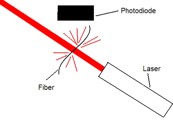
the IR emitters. To solve this problem, an intense and concentrated light source was needed and led to the use of a small laser modified from a laser pointer. In the first test, the laser was aiming at the photodiode with the fiber breaking the beam.
Figure 5.2 Laser / Photodiode Diagram
Figure 5.3 Reflected Laser / Photodiode Diagram
The parallel nature of laser light ensured that when there was no fiber present very little of the laser light would reach the photodiode, however, when a fiber was present the laser would illuminate the fiber and reflected light would reach the photodiode. Initial
experimentation used both a photodiode and a photoresistor incorporated into a simple voltage divider to create a voltage change along with the change in resistance. The photoresistor initially worked better than the photodiode registering a larger voltage change, however the response time was very slow. The photoresistor required a
5.1.2 Final Design
The fiber sensor was designed using a laser positioned perpendicularly to both the fiber direction and the sensor. The fiber would pass through the laser and the light would reflect off of the fiber illuminating the sensor causing a voltage change. Once the
concept of the fiber sensor was developed, a working prototype had to be designed and integrated so that it could control the camera. At the heart of the sensor is the OPT101® photodiode from Burr-Brown, which was chosen due to a good spectral response to the lasers wavelength and an integrated op amp [22]. The spectral response is critical because in order to achieve the largest possible voltage change, the sensor must be
sensitive to the same wavelength of light that the laser is producing. The OPT101® has a wide response band, and while the peak is not at the 630nm wavelength of the laser, there is still an acceptable response to that wavelength [22].
Figure 5.4 Photodiode Spectral Response [22]
circuit without amplification. Shown below is a schematic of the circuit contained within the photodiode.
Figure 5.5 Photodiode Amplifier Circuit [21]
)
(
V
2V
1R
R
V
Fout
=
−
Equation 5.1 Difference Amplifier Equation [5]
A difference amplifier is an op amp, configured to accept two voltages as inputs, that outputs the difference between V2 and V1 multiplied by a constant which is set by the resistors chosen for R and RF. To achieve an acceptable multiplication constant R was
set to 1KΩ and RF was set to 6.2KΩ yielding a multiplication constant of 6.2.
and then dialed back slightly to achieve a value just below the voltage required to trigger the camera. By using a transistor, the required rising edge TTL signal could easily be integrated with the trigger circuit required for the camera as shown in Figure 5.8.
Figure 5.7 Sensor Circuit Diagram
The circuit below came from the camera manual and provides a way to trigger the camera using the rising edge trigger created by the Figure 5.7 circuit. The rising edge trigger will be inverted by the NOT gate which will show a ground on the other side of the circuit. The five volts will now flow through the optoisolator tripping the phototransistor and causing the camera to capture an image. An optoisolator is used to isolate sensitive electronics from potentially harmful voltage or current. Since there is no physical
Figure 5.8 Camera Trigger Circuit [25]
5.1.3 Analysis of Effectiveness
Initial attempts to evaluate the effectiveness of the sensor consisted of manually moving a single cotton fiber into the laser beam. A LED was used to simulate the camera and provide a visual representation of when the camera would be triggered. The sensor was able to reliably detect the presence of a single fiber each time one was present. The next test evaluated the ability of the sensor to detect moving fibers. Once again fibers were moved through the beam manually only this time they were moved quickly. Once again the sensor proved effective and could detect fast moving fibers.
increased brightness. The sensor then was able to effectively detect the presence of each fiber introduced into the system.
5.2 Fiber Transport Enclosure
Once the sensor had been developed and proven effective in detecting fibers, a method was needed to move the fibers from the comber roll, past the sensor and in front of the camera in a reliable and repeatable manner. A variety of ideas were theorized and in the end many were tested leading to an effective method of controlling and distributing fibers to the viewing area.
5.2.1 Method
The new design focuses on controlling the fibers without any physical contact. Suction is a widely utilized method of controlling fibers and was at the heart of all the potential solutions. To ensure the best solution the ideal solution was first theorized and involved the fibers moving through air with no material between the fiber and the camera. This solution proved impractical and further design was needed to arrive at a workable solution. Preliminary designs sought to deliver the fibers to the viewing area unobstructed and thus incorporated a gap between two tubes in the hope the fiber would follow the airstream between the paths as shown in figure 5.9. Relying solely on air to transport the fibers between the input tube and the output tube proved ineffective and therefore a more controlled method was developed. New designs were theorized and tested which incorporated a clear tunnel which would contain the air stream and the fiber. 5.2.1.1 Air Gap
that anything would either obstruct the fiber or interfere with the quality of the image. Two tubes were used with a 1.5” gap between them to ensure that even the longest (1.25”) fibers would not be obstructed by the tubes.
Figure 5.9 Air Gap System
chance that the fibers will cross the imaging area consistently. Another downside is that the fibers would not be contained in a single plane making it difficult to accurately focus the camera resulting in blurry images.
5.2.1.2 Coanda Effect
The next design would utilize the coanda effect to cause the fibers to follow a slightly curved path. The coanda effect is one of the effects airplane wings utilize,
causing the air to follow the curvature of the wing and be directed downward causing lift. In theory, the airstream containing the fiber would follow a curvature providing more control over the fiber resulting in better delivery to the viewing area. The diffusing plate from the backlight would be used as the path for the fibers to follow so that the contrast between the fibers and the background would be as high as possible while also
simplifying the design. Testing once again showed that this method was ineffective and fibers were not able to be controlled effectively.
Theoretically the air would travel over the surface and the coanda effect would cause the air to follow the surface leading toward the tube providing the suction. The theory was sound and if the air speed was high enough the fiber could cross the gap. While the fiber could now be controlled the image of the fiber was very blurry due to the high speed. The image was too blurry to allow effective processing and therefore a fiber control method allowing slower fiber speeds was the focus of a new design.
5.2.2 Enclosed Transport System
which design would provide the best control, while eliminating the possibility that a portion of the fiber would be obstructed from the camera
5.2.2.1 Preliminary Enclosed Fiber Design
The first iteration was simply a tunnel through which the fibers would travel, and an adapter at each end to smoothly transfer the fibers from the comber roll to the
enclosure. This design shown in figure 5.10 was a good start but the machining was very complicated and a simpler design was needed. This simpler design shown in Figure 5.11 would make it much easier to build a prototype to test the theory before machining.
Figure 5.11 Redesigned Enclosure
The transition from input adapter to tunnel is accomplished by a simple angled piece channeling the fiber to the tunnel, where it is sensed and an image is captured. A simple prototype as shown in figure 5.11 was constructed and evaluated to determine if the design would effective deliver the fibers to the viewing area.
5.2.2.2 Preliminary Design Problems
appeared blurry. The design was also too narrow and there was no way to ensure that the fibers would not come in contact with the walls, obstructing sections of the fiber from the camera. The final problem was that the tunnel was not long enough. The camera has a reset time of approximately 8ms meaning that from the time it is triggered there is a delay time of at least 8ms before it can take a picture. To accommodate the inherent camera delay, the tunnel must be longer than the distance a fiber can travel in 8ms ensuring that the entire fiber is captured by the camera.
5.2.2.3 Redesigned Fiber Transport Enclosure
The next iteration shown in figure 5.12 was designed to solve the problems faced by the preliminary design. The tunnel was significantly wider than the first design to eliminate fibers touching the edges of the tunnel. By widening the tunnel the fibers would slow down due to the reduced air speed inside the opening helping to improve image quality. The tunnel was also made longer to account for the reset time needed for the camera.
5.2.2.4 Redesigned Fiber Transport Enclosure Design Problems
The new design did not solve the problems it set out to solve however it did enable a better assessment of the specific problems. While the tunnel was longer the fibers continued to be captured at the end of the enclosure. The position of the fibers was not very consistent and an area containing the majority of fibers could not be pinpointed. The fibers also showed a tendency to move toward the edges of the enclosure creating the possibility that the fibers would either be partially out of frame or come in contact with the edges causing some obstruction. Turbulent flow again was a problem and was especially noticeable at the entrance to the enclosure. The turbulence caused the ends of the fibers to appear blurry on the camera and was also thought to contribute to the fibers proximity to the sides of the enclosure. The turbulent flow was theorized to be caused by the sharp transition from the small volume of the tube to the large volume of the viewing area thus allowing the air to expand quickly, causing turbulence.
5.2.2.5 Redesigned Fiber Transport Enclosure
Figure 5.13 Tapered Contour
5.2.2.6 Redesigned Fiber Transport Enclosure Design Problems
The length chosen for the enclosure worked well, allowing the position of the fibers to be controlled with the air speed and the delay time. The turbulence of the fibers was not significantly decreased and some blur at the tip was noticeable. The turbulence was found to significantly decrease when the air velocity was decreased so reducing turbulence was no longer a significant problem. The number of fibers near or contacting the edges in the viewing area were significantly increased when compared to the previous design. This was a significant problem and attributed to the air following the contour of the enclosure. By gradually widening the enclosure the air, and thus the fiber, can easily follow the contour leading to the edges of the viewing area.
5.2.2.7 Analysis of Design Solutions
With limited ability to predict the behavior of individual fibers in an air stream, the design process benefited significantly from the ability to mock up simple and cheap prototypes to test the different design solutions. The first designs focused on the ideal solutions in which there would be no material between the fiber and the camera ensuring the best image quality possible. This design proved difficult due to the problems
focus shifted to an enclosed design and preliminary prototypes were developed to test each design change ensuring that time and money would not be wasted having flawed designs machined. After much experimentation and observation a final design was decided upon.
5.2.3 Final Design
The final design was simply a slight modification of a previous design with the wide viewing area and no tapered entrance combined with an elongated entrance tunnel as shown in figure 5.14. By controlling the fiber within the tunnel and releasing it into the viewing area from the center there was no chance the fiber would move toward the edge before it was redirected by the suction. The long entry tunnel also gave the camera time to reset before the image was captured allowing the position of the fiber to be controlled by the timing and the airspeed.
5.2.3.1 Theory
Figure 5.14 Final Enclosure Contour
Figure 5.15 Enclosure Design
The prototype was constructed out of polycarbonate and was glued together avoid having to be professionally machined. The final design would require a good deal more
Figure 5.16 Sandwich Design
Figure 5.18 Exploded View
Figure 5.19 Entrance Adapter Top
Figure 5.20 Entrance Adapter Bottom
Figure 5.21 Entrance Adapter Wireframe
provided a smooth transition from the round intake tube to the rectangular tunnel. A smooth transition was important to avoid fiber entanglements or fibers getting stuck which would either increase error due to excess entanglements or cut off flow of the fibers to the viewing area rendering that run useless. Overall, the design was an effective method to deliver fibers to the viewing area in a consistent and controlled manner. 5.2.3.2 Material Selection
When experimenting with preliminary prototypes, a significant number of fibers would stick to the top or bottom of the enclosure due to the static that had developed on the surfaces. This was a major concern for the final design since fibers stuck in the enclosure would cause erroneous readings. This problem had to be completely
eliminated for the machine to be successful. By using a static dissipative acrylic for all of the surfaces, the static was eliminated. While slightly more expensive than normal
acrylic or polycarbonate the cost was not prohibitive and the material proved to be very effective in reducing static and resulted in the problem being completely eliminated.
It was important to have rigidity so that the input and exhaust tubes could be securely mounted to the enclosure and so all of the plastic enclosure pieces could be bolted tightly together ensuring minimal air leaks. An 1/8” aluminum plate was used as a base to provide sufficient rigidity. Aluminum was chosen because of its ease to machine and ability to provide the rigidity needed.
For the adapter shown in figure 5.19, 5.20, and 5.21 delrin was the material of choice. Strength was not important however cost and ease of machining were
5.2.3.3 Final Design Evaluation
The final design was very effective, however, like any design there are opportunities which need to be considered. The first is the tendency for fibers to
occasionally get stuck at the end of the intake adapter. The problem appears to be caused by the gap created when the top and the bottom pieces fit together. The fiber enters the gap and the natural crimp of the fiber causes it to become stuck between the two pieces. The fiber will then flutter in and out of the laser constantly triggering the sensor. This eliminates any chance of synchronizing incoming fibers with the camera which causes all subsequent images to be empty. This problem could be fixed by remachining the adapter pieces with a tighter tolerance, or out of a solid piece. A more robust solution would simply be to move the sensor down the path an inch or so. This way even if a fiber did get stuck it would not be able to trigger the camera eliminating the problem. This would require that a few parts be remade and since the problem is not significant there is not an immediate need to make this design change.
Another problem noticed once images were taken and analyzed was a slight increase in blur caused by the acrylic. Images of fibers within the enclosure were compared to images on top of the enclosure and a 1-2 pixel increase in blur was
The final design effectively solved all of the problems associated with controlling individual cotton fibers and delivering them first past a sensor and into a viewing area in a continuous and repeatable manner. The dimensions of the enclosure ensured the fiber would be controlled and not allowed to contact the edges during imaging while ensuring there was ample time between sensing and imaging for the camera to reset itself and capture the image. The materials chosen eliminated static while providing the clearest image possible to increase the chance of accurate software analysis. The overall design was simple and easy to build and modify while solving the major design criterion associated with the problem.
5.3 Light Source
The backlighting configuration chosen in the final design requires a uniform, strobing light source to provide illumination resulting in a high contrast silhouette of the fiber, optimizing the image for processing. The ability to strobe is required to freeze the motion of the fiber eliminating blur and resulting in a clear image. The camera must trigger the light source in order to synchronize its shutter and the light so that the image is captured when light is triggered and a fiber is present in the viewing area.
5.3.1 Method
the image. When the shutter opens, or in the case of a digital camera, each photodetector is reset and allowed to react to the light reaching it, a voltage proportional to the light at that photodetector is created. At the end of the integration period (when the shutter closes) the camera reads the voltage from each photodetector and relates it to a pixel value between 0 and 255, 0 being black meaning no light reached the pixel and 255 being white meaning that the pixel was saturated with light. If the strobe light is only on for a fraction of the shutter speed of the camera, the only light reaching the camera during the exposure time is that from the strobe along with a small amount of ambient light. Ambient light is reduced and the remaining light reaching the camera is insignificant when compared to the intensity of the strobe. If the strobe has a very short duration, the fiber in the image will only move a very short distance during the time the light is on, creating an image in which the fiber appears to be stationary. Even though the fiber continues moving after the flash no more light reaches the camera and the pixel values remain unchanged. If the strobe duration is too short, or the intensity too low, not enough light will reach the camera causing the image to appear very dark. The goal is to
maximize the intensity and minimize the strobe duration while maintaining the ability to precisely control the strobe and provide a uniform background.
5.3.2 Existing LED Backlight
Tests with the existing strobe showed good results using 50µs to 60µs strobe duration. The images were clear enough to visually inspect but the intensity suffered in the quest for shorter duration and were not able to be processed effectively using the existing software. A thorough search of commercially available backlights was performed and little practical information about luminous intensity could be obtained. Since it was difficult to compare the brightness of the lights and the lights were rather costly, deciding on one was difficult and there was uncertainty as to whether the purchase would lead to the required increase in intensity.
5.3.3 Ultra bright Led Array
To solve the intensity problem, a custom light array was designed and built to provide the required intensity while maintaining the short durations necessary to eliminate blur. LED’s were the focus of the search for a new backlight due to many positive attributes. LED’s are commonly used in both front and backlighting for machine vision applications and have a very long life. LED’s also provide a low voltage and low current lighting solution which simplifies the design while also increasing safety by not using high voltage or high current. Finally and most importantly LED’s can be strobed very fast which ideally suits the current application. A search for ultrabright LED’s was performed and the Luminex Emitter III was clearly brighter than any other LED’s commercially available.
5.3.3.1 Theory
Figure 5.22 Camera Spectral Response [25]
As seen in the graph the highest spectral response occurs at a wavelength of 630nm which fortunately is a wavelength of light that could be chosen for the LED’s. The difficulty with creating an LED array is ensuring that it provides a uniform background for the fiber. If the background is not uniform it is difficult to analyze the image. By using a current limiting LED driver, the current through one or a series of LED’s remains the same while the voltage is changed depending on the number of LED’s being driven, ensuring a uniform intensity from all LED’s on the circuit. The recommended driver was the BuckPuck which could drive 3 LED’s in series and allowed for external triggering [1]. The strobe duration was related to the trigger signal in that the light would stay on as long as the signal was high. However, the minimum strobe duration was approximately 50µs which was well within the range determined using the original strobe light. The LED drivers were equipped with a control pin which allowed relatively simple
![Figure 2.2 CMOS Chip Diagram (Reproduced From [20])](https://thumb-us.123doks.com/thumbv2/123dok_us/1237438.1156287/16.612.92.521.78.325/figure-cmos-chip-diagram-reproduced.webp)
![Figure 5.5 Photodiode Amplifier Circuit [21]](https://thumb-us.123doks.com/thumbv2/123dok_us/1237438.1156287/57.612.233.382.130.286/figure-photodiode-amplifier-circuit.webp)
