A Plastic Injection Molding Process Characterisation Using Experimental Technique: A Case Study

(1)

Jurnal Teknologi, 41(A) Dis. 2004: 1–16 © Universiti Teknologi Malaysia

A PLASTIC INJECTION MOLDING PROCESS

CHARACTERISATION USING EXPERIMENTAL DESIGN TECHNIQUE: A CASE STUDY

SHAIK MOHAMED MOHAMED YUSOFF1, JAFRI MOHD. ROHANI2,

WAN HARUN WAN HAMID3 & EDLY RAMLY4

Abstract. This paper illustrates an application of design of experimental (DOE) approach in an industrial setting for identifying the critical factors affecting a plastic injection molding process of a certain component for aircond assembly. A critical to quality (CTQ) of interest is reducing process defects, namely short-shot. A full factorial design was employed to study simultaneously the effect of five injection molding process parameters. The five process parameters are backpressure, screw rotation speed, spear temperature, manifold temperature, and holding pressure transfer. Finally, the significant process parameters influencing the short-shot defect have been found. Empirical relationship between CTQ and the significant process parameters were formulated using regression analysis.

Keywords: Design of experiments, injection molding, analysis of variance (ANOVA), regression analysis

Abstrak. Kertas kerja ini mengillustrasikan applikasi reka bentuk eksperimen dalam industri pemprosesan suntikan plastik untuk salah satu komponen penyaman udara. Objektif utama reka bentuk eksperimen ini ialah untuk mengenal pasti parameter mesin suntikan plastik dan seterusnya menentukan paras optima mesin yang mempengaruhi karekteristik output, iaitu short-shot. Reka bentuk factorial penuh telah dipilih untuk kajian ini dengan mengenal pasti lima mesin parameter, iaitu backpressure, screw rotation speed, spear temperature, monifold temperature, dan holding pressure transfer. Keputusan kajian telah dapat mengenal pasti mesin parameter yang mempengaruhi karekteristik

output dan mesin parameter signifikasi tersebut telah dianalisa melalui model regrasi.

Kata kunci: Reka bentuk eksperimen, mesin suntikan plastik, analisa varian, analisa regrasi

1.0 INTRODUCTION

There are mainly three principals of Design of Experiments (DOE) methods in practice today. They are the Classical or Traditional methods, Taguchi methods, and Shainin methods. Sir Ronald Fisher, who applied DOE to agricultural problem in 1930, applied

1,2&3

Unit Kejuruteraan Kualiti, Jabatan Kejuruteraan Pengeluaran & Industri, Fakulti Kejuruteraan Mekanikal, Universiti Teknologi Malaysia, Skudai, Johor. Email: [email protected]

4

(2)

the traditional method to his work [1]. Dr Taguchi of Japan refined the technique with the aim of achieving robust product design against sources of variation [2]. The Shainin method was designed and developed by consultants. Dorian Shainin used a variety of techniques with major emphasis on problem solving for characterising product development [3]. Experimental design techniques are a powerful approach in product and process development, and they have an extensive application in the engineering areas. Potential applications include product design optimisation, process design development, process optimisation, material selection, and many others. There are many benefits gained by many researchers and experimenters, from the application of experimental techniques [2].

In an injection molding process development, DOE can be applied in identifying the machine process parameters that have significant influence in the injection molding process output [2]. The easiest way to do the set-up on the injection-molding machine is based on the machine set-up operator or technician’s experience, or trial and error method. This trial and error method is unacceptable because it is time consuming and not cost effective. Common quality problems or defects that come from an injection molding process include voids, surface blemish, short-shot, flash, jetting, flow marks, weld lines, burns, and war page. The defects of injection molding process usually arise from several sources, which include the preprocessing treatment of the plastic resin before the injection molding process, the selection of the injection-molding machine, and the setting of the injection molding process parameters. The objective of this paper is to obtain the optimal setting of machine process parameters that will influence Critical to Quality (CTQ) and subsequently, reduce the process defects.

2.0 CASE STUDY

Due to a non-disclosure agreement between the company and the authors, certain information relating to the company cannot be revealed, however, the data that has been collected for the experiment is real. The following case study was carried out at a plastic injection molding process department in an air-conditioning assembly company. One critical component in an air-conditioning assembly, which is the main focus in this study is the cross flow fan. Since this cross flow flan is a critical component in the company’s latest new product introduction, high process defects of cross flow fan from the injection molding process is the company’s main concern. The data collection was limited to 2 months because the line was just being set-up and the product has just been introduced into the market in October 2001.

Figures 1 and 2 show that for two consecutive months of November and December 2001, line number 26 contributed to the highest cross flow rejection, with an average of about 30 % rejection for that 2-months interval.

(3)

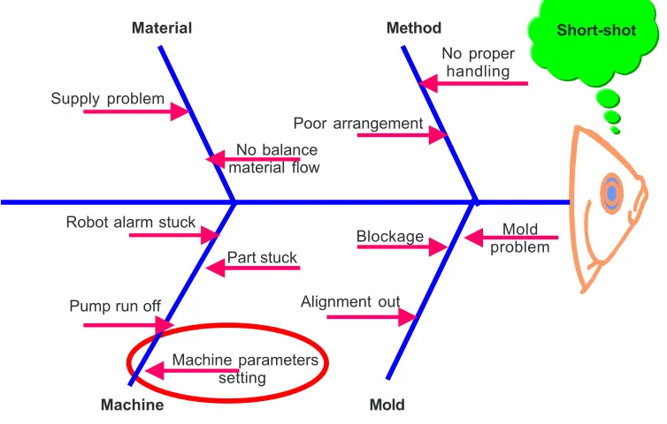
types of defects were due to shot. The combined 2-month average of the short-shot defects were about 47 % of the total types of defects in the cross flow fan rejection. An example of short-shot defect is shown in Figure 5. It is caused by the phenomenon of cooling and solidifying of resin before it fully fills up the mold cavity. This usually occurred in the beginning of the injection molding process. The team conducted a brainstorming session to find the root cause of the short-shot defects, and summarized the outcome in a cause and effect diagram in Figure 6.

0 5000 10000 15000 20000 25000 30000 35000

1 2 3 4 5 6 7 8 9 ₁₀ ₁₁ ₁₂ ₁₃ ₁₄ ₁₅ ₁₆ ₁₇ ₁₈ ₁₉ ₂₀ ₂₁ ₂₂ ₂₃ ₂₄ ₂₅ ₂₆

LINES OR MACHINE

REJECTION OUTPUT

Figure 1 Total cross flow fan rejection for the month of November 2001 [4]

Rejection

Lines or machine

Fan output

Output

0 5000 10000 15000 20000 25000 30000 35000 40000

1 2 3 4 5 6 7 8 9 ₁₀ ₁₁ ₁₂ ₁₃ ₁₄ ₁₅ ₁₆ ₁₇ ₁₈ ₁₉ ₂₀ ₂₁ ₂₂ ₂₃ ₂₄ ₂₅ ₂₆

LINES OR MACHINE

REJECTION OUTPUT

Figure 2 Total cross flow fan rejection for the month of December 2001 [4]

Fan output

Output Rejection

(4)

2.1 Investigation on Causes of Problem

From the cause and effect diagram shown in Figure 6, the team has classified the root cause into four major categories, namely; material, machine, method, and mold. For the method category, the problem could be due to improper material handling by the operator. Meanwhile, from the material side, the problems could be due to imbalance material flow and material quality problem that came from the supplier. From the

Figure 3 Total defects in Line 26 for the month of November 2001 [4]

0 500 1000 1500 2000 2500 3000 3500 4000 4500 0 10 20 30 40 50 60 70 80 90 100 Percentage T otal defect

Type of defects

Dented Blanching out Oily Flowmark Welding out Sinmark Broken Jumping Scratches Water leaking Vibration Silver Crack Others Dirtmark Short-shot

Figure 4 Total defects in Line 26 for the month of December 2001 [4]

0 500 1000 1500 2000 2500 3000 3500 4000 4500 5000 0 10 20 30 40 50 60 70 80 90 100 Percentage T otal defect

Type of defects

(5)

machine side, the problem could be due to three major causes that affected the process and contributed to short-shot, namely; part stuck, robot alarm error, and pump run off. From the mold side, the problems could be due to mold problem, blockage, and mis-alignment.

Figure 5 Example of short-shot defect

Figure 6 Cause and effect diagram for short-shot problem

SHORT-SHOT

Machine

Machine parameters setting

Pump run off Alignment out

Material Method

No proper handling

Supply problem

Poor arrangement

No balance

materialflow

Robot alarm stuck

Blockage Mold

problem Part stuck

Short-shot

(6)

Finally, from the machine perspective, the team decided that the machine parameter setting could be the key to overcoming the short-shot problem. Based on the above four major categories, the team decided to work on machine parameter setting first and had chosen design of experiment (DOE) as a methodology to reduce short-shot problem. The case study was carried out by the following general steps in classical experimental design methodology.

2.1.1 Step 1: Identify The Objective/Goal Of The Experiment

The goal of the experiment is to determine the most significant factors affecting CTQ and subsequently, reducing the short-shot defects.

2.1.2 Step 2: Identify The Input Parameters And Output Response

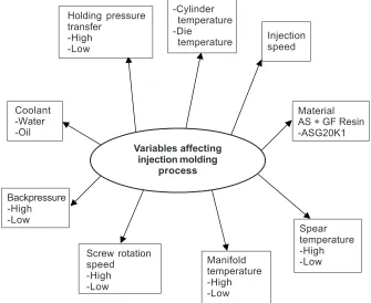
Based on the process knowledge experience from the process engineer, literature review, and machine supplier, the variables or input parameters that will be influencing the short shot defects are as shown in Figure 7. Based on the advice of the company’s process engineer, literature review, machine history, maintenance report, and material study, the team decided to select the backpressure, spear and manifold temperature, holding pressure transfer, and screw rotation speed as input parameters.

Variables Affecting Injection Molding Process Coolant -Water -Oil Material AS + GF Resin -ASG20K1 Manifold temperature -High -Low Spear temperature -High -Low Backpressure -High -Low Injection speed -Cylinder temperature -Die temperature Variables affecting injection molding process Screw rotation speed -High -Low Holding pressure transfer -High -Low

(7)

The team decided to use the weight of the blade of cross flow fan for the output response. Based on the study, the weight is closely related to the short-shot problem. The range of blade with weight between 51.0 and 53.0 gram does not have short-shot problem.

2.1.3 Step 3: Select Appropriate Working Range For Input Parameters

An initial trial of experiment was performed to find the feasible input parameters’ working range. If back pressure, screw rotation speed, holding pressure transfer, manifold, and spear temperature were set incorrectly, the types of defects shown in Figure 3 could occur. Table 1 shows the test range for the input parameter levels in the injection molding process.

2.1.4 Step 4: Select The Factors And Its Level

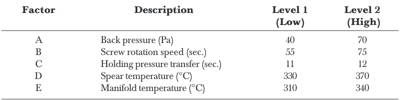
Based on initial and pilot experiment data, the main factors such as backpressure, holding pressure transfer, screw rotation speed, and spear and manifold temperature were selected. The appropriate working range was selected based on this pilot experiment. The team tested this level on the injection-molding machine before selecting the best parameter levels for the full-fledged experiment. Table 2 is the selected parameter levels for this injection molding process.

Table 2 The selected parameters and its chosen level

Factor Description Level 1 Level 2

(Low) (High)

A Back pressure (Pa) 40 70

B Screw rotation speed (sec.) 55 75

C Holding pressure transfer (sec.) 11 12

D Spear temperature (°C) 330 370

E Manifold temperature (°C) 310 340

Table 1 Test range for input parameters

Factor Description Test range - Min/Max

A Back pressure (Pa) 45 - 70

40 - 65

B Screw rotation speed (sec.) 65 - 75

55 - 70

C Holding pressure transfer (sec.) 11 - 12

D Spear temperature (°C) 330 - 350

340 - 370

E Manifold temperature (°C) 310 - 330

(8)

2.1.5 Step 5: Full Factorial Experimental Designs

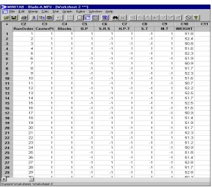
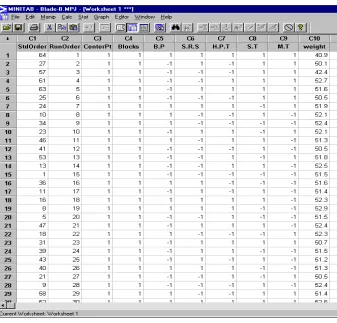
The choice of the experimental design has an impact on the success of the industrial experiment. It also involves other considerations such as the number of replicates and randomization. For this study, five independent factors (each at two levels) are to be studied, thus, a full factorial experimental design was used and a total of 32 experimental runs were required. Each run will require 2 replicates, giving a total of 64 experiments. Experimental design matrix was constructed, so that, when the experiment was conducted, the response values could be recorded on the matrix.

For each injection process, 4 blades will be produced from 4 different mold cavities. The weight results in Figure 8 are from mold cavity 1 and 2 and the weight results in Figure 9 are from mold cavity 3 and 4.

Figure 8 Pareto chart of standardized effect

Figure 9 Main effect for analysis B

A A

51.7

51.5

51.3

51.1

50.9

M.T.

(9)

2.1.6 Step 6: Dry Runs Of The Planned Experiments

Each combination of factors was run on the machine for a short duration to ensure successful runs in the full-fledged experiment. The selected factor with its levels is found to be suitable for experimentation.

2.1.7 Step 7: Full Fledged Experiments

The experiment was conducted based on the prepared experimental design matrix in Step 6. The resulting response values are shown in Tables 3 and 4. The weight of blade was measured by using digital weight machine. The actual experiment was conducted in the factory with some help from the staff of the company, taking two working days to be completed.

(10)

2.1.8 Step 8: Analyze The Experimental Result

The goal of the experiment is to establish the “optimum” setting for injection molding process to reduce the short-shot defect. The experimental data was analyzed using the Statistical Minitab Version 13 software. The data was divided into two parts based on the mold cavity location. The analysis was done based on the cavity location.

(1) Analysis A

Table 3 shows some portion of the experimental runs and recorded output response values of weight. Pareto chart is used to reveal the sequencing of the process parameters significant effects. The Pareto chart in Figure 8 shows that the most significant factors and interacting are A, CD, AC, and AE. It further assists the user in finding the real effects. The effects are listed from the largest to the smallest. Backpressure (A) is the most significant parameter at α = 0.1.

(11)

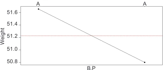
Figure 10 shows the factors that affect the response. The graph shows that backpressure has a negative slope, which means that when the level changes from high to low, the output response will increase steadily. Interaction exists when the level of some other factor influences the nature of the relationship between the response variable and certain factor. If two lines are shown with sharply different slopes, it is considered that interactions exist between the two factors.

Figure 10 Main effect for analysis A

Weight

Figure 11 Interaction plot for analysis A

Figure 11 shows that interaction exists between C and D, which are holding pressure transfer and spear temperature.

(2) Analysis B

The Pareto chart in Figure 12 graphically shows that the most significant factors and interacting are E, AB, BC, and AC. It further assists the user in finding the real effects. The effects are ranked in order from largest to smallest. Manifold temperature E is the largest and backpressure × holding pressure transfer is the smallest at a = 0.1.

51.6

50.8 51.0 51.2 51.4

B.P

51.5 51.0 50.5

A A A A A A

(12)

Figure 12 also shows that factor E that is manifold temperature, have the steep negative slope.

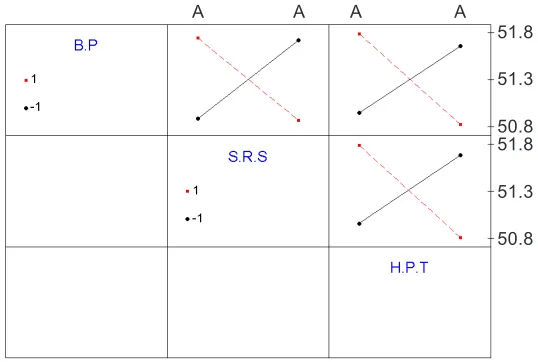
Interaction exists when the level of some other factor influences the nature of the relationship between the response variable and certain factor. Figure 13 shows the interaction plots, namely pressure transfer (C) × screw rotation speed (B), back pressures (A) × holding pressure transfer (C), and screw rotation speed (B) × holding pressure transfer (C) interactions.

Figure 12 Pareto chart of standardized effect

Figure 13 Interaction plot for analysis B

A A A A

51.8

51.3 51.8 50.8 51.3

(13)

The next step is to identify the optimal setting for analysis A and B. Optimal setting was selected based on low (–) or high (+) settings. The factors have been situated in the main effect and interaction graph. From analysis A and B, the optimal setting is shown in Tables 5 and 6. Table 7 shows the final optimal setting obtained from the combination of analysis A and B.

Table 5 Optimal setting for analysis A

Factors Description Value Optimal setting

B.P Back pressure 40 Pa Low (–)

H.P.T Holding pressure transfer 11 sec. Low (–)

S.T Spear temperature 370°C High (+)

M.T Manifold temperature 310°C Low (–)

S.R.S Screw rotation speed 55 sec. Low (–)

Table 6 Optimal setting for analysis B

S.T Spear temperature 330°C Low (–)

S.R.S Screw rotation speed 75 sec. High (+)

Table 7 Final optimal setting

S.T Spear temperature 370°C High (+)

S.R.S Screw rotation speed 75 sec. High (+)

Regression analysis

(14)

(+ve) symbol were identified from the main effect and interactions graph. The postulated model for predicted weight of blade (output response) based on regression analysis:

Weight predicted value (g) for analysis A = Constant - BP + BP × HPT + BP × MT

– HPT × ST

= 51.2266 – 0.4266 (-) + 0.3609 (-) (-) + 0.3578 (-) (-) – 0.3828 (-) (+)

= 52.8 gram

Table 8 Estimated effects and coefficients for weight analysis A (coded units)

T e r m E f f e c t Coef SE Coef T P

Constant 51.2266 0 . 2 1 2 9 2 4 0 . 6 4 0.000 B . P - 0 . 8 5 3 1 - 0 . 4 2 6 6 0 . 2 1 2 9 -2.00 0.051 S.R.S - 0 . 1 5 3 1 - 0 . 0 7 6 6 0 . 2 1 2 9 -0.36 0.721 H.P.T 0 . 5 2 8 1 0 . 2 6 4 1 0 . 2 1 2 9 1.24 0.221 S . T 0 . 4 0 9 4 0 . 2 0 4 7 0 . 2 1 2 9 0.96 0.341 M . T 0 . 5 9 6 9 0 . 2 9 8 4 0 . 2 1 2 9 1.40 0.167 B.P*S.R.S 0 . 0 1 5 6 0 . 0 0 7 8 0 . 2 1 2 9 0.04 0.971 B.P*H.P.T 0 . 7 2 1 9 0 . 3 6 0 9 0 . 2 1 2 9 1.70 0.096 B . P * S . T 0 . 6 4 0 6 0 . 3 2 0 3 0 . 2 1 2 9 1.50 0.139 B . P * M . T 0 . 7 1 5 6 0 . 3 5 7 8 0 . 2 1 2 9 1.68 0.099 S.R.S*H.P.T 0 . 2 3 4 4 0 . 1 1 7 2 0 . 2 1 2 9 0.55 0.585 S.R.S*S.T -0.0469 - 0 . 0 2 3 4 0 . 2 1 2 9 -0.11 0.913 S.R.S*M.T -0.0219 - 0 . 0 1 0 9 0 . 2 1 2 9 -0.05 0.959 H.P.T*S.T -0.7656 - 0 . 3 8 2 8 0 . 2 1 2 9 -1.80 0.078 H.P.T*M.T -0.4031 - 0 . 2 0 1 6 0 . 2 1 2 9 -0.95 0.348 S . T * M . T - 0 . 3 3 4 4 - 0 . 1 6 7 2 0 . 2 1 2 9 -0.79 0.436

Table 9 Estimated effects and coefficients for weight analysis B (coded units)

Term Effect Coef SE Coef T P

(15)

Weight predicted value (g) for analysis B = Constant - MT - BP × SRS - BP × HPT

– SRS × HPT

= 51.3078 – 0.4359 () 0.4297 (+) () -0.4203 (+) (-) – 0.4266 (+) (-) = 53.0 gram

2.1.9 Step 9: Verification And Validation

Based on the “optimum setting” as shown in Table 7, the team ran some verification test shot to compare between the actual and predicted results based on regression analysis. Confirmation runs were carried out to check the reproducibility and predictability of result. This ensures that the “optimum setting” is able to predict the output response.

To do this verification run, five experimental shots were carried out based on the settings in Table 7. The results of the confirmation runs are shown in Figure 14.

Figure 14 shows the comparison between the actual and predicted value of blade weight for three different settings. It seems that for the three different settings, there are not much difference between the predicted and actual value. The results are acceptable as they are still within the customer specification limits of between 51 and 53 gram, and no short-shot defects were found for all verification run.

Figure 15 shows the standard deviation and percentage error that occurred for three different settings. All settings showed an experimental error of less than 2%, less than the requirements of reproducibility, which should be less than 10% [1].

Figure 14 Difference between actual and predicted value for respected setting

52.8

53 53

52.34

52.05

51.955

51.4 51.6 51.8 52 52.2 52.4 52.6 52.8 53 53.2

Setting A Setting B Setting C

Predicted Actual

Predicted

Blade weight

Actual

Setting B

Setting A Setting C

(16)

3.0 CONCLUSION

The classical full factorial of DOE approach has been applied to the injection molding process to reduce the short-shot defect in blade. Five controllable factors chosen for the experiment are backpressure, holding pressure transfer, spear temperature, manifold temperature, and screw rotation speed. The significant factors for analysis A have been identified, and they were backpressure, backpressure × holding pressure transfer,

holding pressure transfer × spear temperature, and backpressure × manifold

temperature. Meanwhile for analysis B, the significant factors were manifold

temperature, backpressure × screw rotation speed, screw rotation speed × holding

pressure transfer, and backpressure × holding pressure transfer. The verification

experiments were conducted and the errors between the actual and predicted value of blade weight were less than 2% and no short-shot defect was found.

REFERENCES

[1] Antony, J. 2001. Improving the Manufacturing Process Using Design of Experiments, a Case Study.

International Journal of Operations and Production Management. 21 (5).

[2] Antony, J., S. Warwood, K. Fernandes, and H. Rowlands. 2001. Process Optimization Using Taguchi Methods of Experimental Design. Work Study. 50 (2).

[3] Kumar, A., J. Motwani, and L. Otero. 1996. An Application of Taguchi’s Robust Experimental Design Technique to Improve Service Performance. International Journal of Quality and Reliability Management. 13 (4).

[4] Shaik Mohamed Mohamed Yusof. 2002. Final Year B. Eng. Project. Universiti Teknologi Malaysia.

0.14 0.186 0.165

0.87

1.79

1.97

0 0.5 1 1.5 2 2.5

Setting A Setting B Setting C

Std. Deviation % Error

Figure 15 Differential std. deviation and percentage error between each setting

Std. dev & % error

Setting B

Setting A Setting C