COMPARATIVE EVALUATION OF TURBULENCE MODEL FOR
BUOYANCY DOMINATED FLOW
B.Gera, P.K.Sharma, R.K.Singh, K.K.Vaze
Reactor Safety Division, Bhabha Atomic Research Centre, Mumbai, INDIA-400085 E-mail of corresponding author: [email protected]
ABSTRACT
The effect of buoyancy on turbulence is important for buoyancy-driven flows for the calculation of the buoyancy generation of turbulent kinetic energy. This effect concerns an increase of the turbulence level in unstably stratified situations and suppression of turbulence production in stably stratified flow regions. Most of the reactor safety related problems i.e. hydrogen distribution, fire propagation, moderator flow distribution, passive decay heat removal, thermal discharge in large water body involves buoyancy dominated turbulence. The standard k-ε model does not include the effect of buoyancy. In order to understand the various turbulence modeling approaches for buoyancy related aspects an in-house CFD code has been developed and various turbulence models has been incorporated. The most commonly used assumption is simple gradient diffusion hypothesis (SGDH) to model the buoyancy source term. However, with this approach the effect of buoyancy on turbulence is substantially underestimated. In order to overcome this problem, buoyancy terms based on the generalized gradient diffusion hypothesis (GGDH) have also been incorporated in the k-ε turbulence model. A hybrid models called partially-averaged Navier-Stokes (PANS) method was also used with the above hypothesis (SGDH, GGDH). All above turbulence models have been used to simulate a 2D axisymmetric buoyant turbulent thermal plume problem under steady state and their performances against each other were compared.
INTRODUCTION
Most of the engineering flows are turbulent. The mathematical modeling of turbulent flows is important in a large number of industrial applications. Currently Reynolds-averaged Navier Stokes (RANS) approach is widely used for the solution of turbulent flows, although approaches based on large-eddy simulation (LES) are increasingly used as significant computing resources become more readily available. In the RANS approach the time averaged transport equation is used, the averaging process creates additional terms, which need to be model for closure problem. Based on RANS approach various models have been developed based on Boussinesq assumption, which relates the Reynolds stresses to the mean velocity gradient via a turbulent viscosity. Additional transport equations are solved and based on their numbers these models are broadly classified as zero-, one-, and two-equation models. Models are available which solves the transport equations for Reynolds stress directly and gives second-moment closure. These models are computationally more expensive and less robust and have consequently found less widespread application. The Boussinesq-based two-equation models have demonstrated a good balance between accuracy and efficiency. In particular, the k-ε turbulence model of Launder and Spalding [1] has been widely adopted, where transport equations are solved for the turbulent kinetic energy (k) and the rate of dissipation of the turbulent kinetic energy (ε). The standard k-ε model [1] is widely used but is not capable of properly capturing the generation of buoyancy induced turbulence and its dissipation and suitable modifications have been proposed.
GGDH gave significantly improved results. Yan and Holmstedt [5] investigated these terms and found optimized values for the empirical constants when applied to a thermal plume.
The thermal plume represents an important benchmark simulation for any buoyant flow code as well as being a relevant flow in its own right, for example, in atmospheric simulations and fire simulations. Considerable experimental work has been carried out in this area, against which it is possible to validate turbulence models. The experimental results before 1980 have extensively been compiled by [3]. Various other experimental results have been compiled [8-10] give excellent database for code validation. This article investigates the performance of various turbulence models for prediction of velocity along the plume centerline.
EXPERIMENTAL RESULTS SELECTED FOR COMPARISON
The standard k-ε model without considering buoyancy over predicts the velocity along the plume centerline since the turbulent kinetic energy generated by buoyancy is not modeled that leads to underestimation of the width of the plume. Corrections are required by tuning the turbulent viscosity coefficient and the effective Prandtl number; the two parameters contained in the k-ε model, thereby reported agreement is improved [11]. CFD simulation is conducted by way of the k-ε models in both incompressible and simplified compressible forms to examine the prediction accuracy for practical applications by comparing numerical results with experimental data [12-13]. It was found that both computed velocity and buoyancy forces overshoot experimental results in the center of a plume. Further, by developing a modified k-ε model incorporating buoyancy-induced anisotropy effects of turbulence validate the model was validated against several flow situations. With the modified model, buoyancy flows can be computed with a sufficient accuracy.
So far, concerning the way corrections are applied against experimental data of thermal plumes, [11] propose tuning the empirical coefficients in the standard k-ε model, while [12-13] propose modified k-ε models. The accuracy of the standard k-ε model, when applied to free plumes under situations found in the fire smoke movement, is examined by comparing results with experimental data (correlations of Yokoi available from [13]). Yokoi determined velocity at any arbitrary location in a rising current as follows:
) 4617 . 1 exp( * ) 1077 . 0 3990 . 0 9174 . 0 1 ( ] [ * 833 .
0 1/3 4/9 1/3 ζ3/2 ζ3 ζ9/2 ζ3/2
ρ + + + − = − − Z C T C gQ w p
(1)
where ζ =r/(ZC2/3)
,
wis velocity in the vertical (z) direction (m/s), is heat release rate (J/s),heat capacity at constant pressure (J/kg-K),
Q Cp
ρ fluid density (kg/m3), Tfluid temperature (K), C constant, Zis z -coordinate (m) and ris radial-coordinate (m). In Yokoi’s experiments, agreement was attained at = 0.062 for a
point heat source and =0.1 for a circular heat source for a circular heat source with a finite radius. For a circular heat source, the above equation is valid along the height in the range of 4 to 10 times radius of the heat source. The Yokoi formula is thought to possess a high reproducibility. Since basis equations—derived through dimensional analysis of the governing equations for axisymmetric plumes embedding the turbulent diffusion coefficient based on the mixing length of turbulence—have fitted firmly to experimental data [13].
3 / 2 C 3 / 2 C TURBULENCE MODEL
The geometry used for computation is shown in Fig. 1. The governing equations for 2D axisymmetric flow are as written below. The general transport equation for variableφ
is
ρφ div ρφu div φgrad φ Sφ
t + = Γ +
∂ ∂ )) ( ( ) ( ) ( r
(2) This can be written as follows for 2D axisymmetric flow
ρφ ρ φ ρ φ φ φ φ φ Sφ r r r r z z r v r r z u
t ∂ +
∂ Γ ∂ ∂ + ∂ ∂ Γ ∂ ∂ = ∂ ∂ + ∂ ∂ + ∂ ∂ ) ( 1 ) ( ) ( 1 ) ( ) ( (3)
where ρ is density of mixture (kg/m3),
t is time (s), , are axial and radial component of velocity
(m/s),
u v
z, r are axial and radial coordinate direction, Γφ is diffusion coefficient for variable φ and is source term for variable
φ S
φ.
For Z-momentum φ=u and Γφ =μeff =μ+μt and
ref g z
v eff r r r z u eff z z p
Sφ (μ ) 1 (μ )−(ρ−ρ )
∂ ∂ ∂
∂ + ∂ ∂ ∂
∂ + ∂ ∂ −
= (4)
Where μ is dynamic viscosity (Ns/m2)
t
μ is turbulent viscosity, is effective viscosity, is dynamic pressure and
eff
μ p
g is acceleration due to gravity (9.81 m/s2).
For R-momentum φ=v and Γφ =μeff =μ+μtand
22 ( ) 1 ( ) r v eff r r r r u eff z v eff r r p S
∂ ∂ ∂
∂ + ∂ ∂ ∂
∂ + ⎟ ⎠ ⎞ ⎜ ⎝ ⎛ − ∂ ∂ −
= μ μ μ
φ (5)
For Energy φ=T and Γφ =k/Cp +μt /Prt and Sφ =0
Fig. 1: Computational domain along with boundary conditions
Different turbulence models based on the Reynolds stresses modeling; turbulent heat flux and turbulent diffusion flux are proposed to close the set of equations. Since the turbulent transport processes depend on the geometry, fluid properties and flow pattern, empirical parameters are used. However, the values are valid only for certain flow, or at some range of the flows. In fact, universal turbulence models for buoyancy dominant flow simulations are absent and the range of validity is problem dependent. Isotropic turbulence models are derived by assuming that the turbulent viscosity is isotropic. The ratio between Reynolds stress and mean rate of deformation is the same in all directions. Analogy between the action of viscous stresses and Reynolds stresses on the mean flow is applied. Transport of heat, mass and other scalar properties can be modeled in a similar manner in terms of the turbulent diffusivity. Two turbulence models were tested in this paper with predicted results on air flow compared with the experimental results on buoyant plume:
• Standard k-ε model with buoyancy modification with SGDH and GGDH
• Partially Averaged Navier-Stokes (PANS) with buoyancy modification with SGDH and GGDH
Standard k-ε model with buoyancy modification with SGDH and GGDH
The standard k-ε model is most widely used turbulence model in most CFD programs for studying industrial flow. This model is applicable for wide ranges of fluid flows and does not require extensive computer resources. Two additional transport equations are solved one for turbulent kinetic energy k and its dissipation rate ε. For modeling buoyancy induced turbulence additional term is added to these equations. There are two arguments on how buoyancy would affect the source terms in the k and the ε equations:
• Buoyancy gives additional sources in both the k and the ε equations.
• Buoyancy affects the source items in k equation only, it is not important or there are insufficient reasons for including the buoyancy in the source terms of the ε equation.
ε μ ρ
μt = C k2 (6)
Where is turbulent kinetic energy (mk 2/s2) and ε is turbulent dissipation rate (m2/s3 and is an empirical constant
.
μ C
For turbulent kinetic energy φ=k and Γφ =μ+μt/Prk
Sφ =Gk+GB−ρε (7) Where is turbulent Prandtl number for kinetic energy, is generation term for turbulent kinetic energy due to the mean velocity gradients and is generation term for turbulent kinetic energy due to buoyancy.
k
Pr Gk
B
G
For turbulent dissipation rate φ =ε and Γφ =μ+μt/Prε
k C f R C B G k G k C S 2 2 ) 3 1 )( )( / ( 1 ε ρ ε
φ = + − − (8)
Where Prt , Prk , Prε , C1 , C2and C3 are empirical coefficients whose standard values were taken and
{2[( )2 ( )2 ( )2] ( )2}
z v r u r v r v z u t k G ∂ ∂ + ∂ ∂ + + ∂ ∂ + ∂ ∂
=μ (9)
And the term GB has been modeled by two hypotheses SGDH and GGDH as described later.
Partially Averaged Navier-Stokes (PANS) with buoyancy modification with SGDH and GGDH
The PANS model [14-15] resolves the large unsteady fluctuations through a partial averaging concept, whose extent is determined by fk and unresolved dissipation rate fε. The model equations used for and k ε are given by
For turbulent kinetic energy φ=k and Γφ =μ+μt/Prk
(10) k L c B G k G
Sφ= + −ρ(ε+ε )+
For turbulent dissipation rate φ=ε and Γφ =μ+μt/Prε
) 2 2 ( 2 2 2 * 2 ) 3 1 )( )( / ( 1 1 j x i u t k f C f R C B G k G k f C S ∂ ∂ + − − + = ρ μμ ε ρ ε
φ (11)
The coefficient * differentiates the PANS model from the baseline RANS model.
2 C
1 ( 2 1)
*
2 C C
f f C
C = + k −
ε
(12)
The value of fε is taken as 1.0 and the coefficientsC1, C2, Prk, Prε are same as the parent RANS model. C1=1.44, C2=1.92, Prk=1.0, Prε=1.30 (13) And the term GB has been modeled by two hypotheses SGDH and GGDH as described in next subsections.
Simple Gradient Diffusion Hypothesis (SGDH)
( ) 2
1
Pr z g
p z t t B
G + ∞
∂ ∂ ∂ ∂ − = ρ ρ ρ μ (14)
Generalized Gradient Diffusion Hypothesis (GGDH)
( ' ' )( ) 2 Pr 2 3 g j x p k x k u j u k t t B
G + ∞
GENERAL DESCRIPTION OF THE PROBLEM AND NUMERICAL DETAILS
The computations were carried out for a reported experiment. In the experiment the heated plume was generated from a circular source of radius ( ) =0.1875 m by providing a heat flux of 8637.8 kW. A large computational domain was used with radius 40 in radial direction and 100 in axial direction. The axisymmetric, incompressible, steady momentum, energy, turbulence and continuity equations were solved using the in-house computational fluid dynamics (CFD) code based on the well-established pressure-based finite-volume methodology using Patankar’s SIMPLE algorithm [16]. Interpolation to the cell faces for the convective terms was performed using a second-order power law scheme. Second-order central differencing was used for the diffusive terms. Staggered scheme of solution was used in which fluid velocities were calculated at cell face and scalars such as pressure, temperature and turbulent quantities were evaluated at cell centre. The equations were iteratively solved using Gauss-Seidel method. Under-relaxation was set as 0.1 for momentum and 0.3 for other equations. The convergence criterion was set 10-5 based on overall mass residual. Each simulation required approximately 2 hrs run time on a P-IV machine with 4GB RAM. A non-uniform grid system was employed for mesh generation. The computational domain was divided in 100X50 grids. In axial direction grid was made fine near heat source and coarser away from the heat source. In radial direction uniform grid was employed up-to heat source region after that grid was made non-uniform coarser towards outer radius.
0 r
0
r r0
RESULTS AND DISCUSSIONS
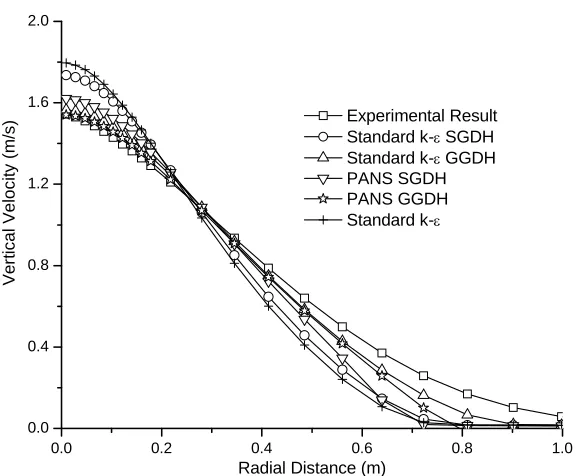
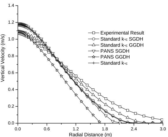
The model was used to predict the performance behaviour of the two turbulence model with two type of buoyancy modification for simulation of buoyant plume. The radial profile of vertical velocity was computed at height 10 , 20 , 40 and 60 . The results of present computation are shown from Fig. 2-5. The computation was also carried out with standard k-ε model without buoyancy modification and result of this is also plotted along with other results. All these figures show that the SGDH model shows no or little improvement on the standard k-ε
model. This is because the value of the term modeled by SGDH is small. This is contrary to results given by [2-3], which show the SGDH to be a great improvement on the standard k-ε model. This could be due to the method of evaluation of spread rates. If the spread rates are measured from the source, then there is the appearance of good improvement. The effect of the SGDH model is for the plume to widen rapidly at the source before settling into the self-similar region, where the spread rate is not altered by the SGDH model as compared to the standard k-ε model. It is clear from the results shown in Fig. 2-5 that the GGDH models gave the most significant increases in spread rates. Conversely, the SGDH, showed little increase on standard k-ε (the unmodified k-ε model), indicating the significance of the GGDH model assumption.
0
r r0 r0 r0
B
G
The spreading rate of a vertical thermal plume is of critical importance. The results of present computation are promising and agree well with experimental data. Computation was also performed using the standard k-ε model and the velocity profiles at various heights were predicted are also shown in Fig. 2-5. One can clearly see that the standard k-ε model seriously under predicts the spreading rates of the thermal plume. In the k-ε model the turbulent transport is closely related to the turbulent transport coefficient which is proportional to and inversely proportional to the turbulent Prandtl number. One may be able to fit specific experimental data by simply adjusting the constants and turbulent Prandtl number as Nam and Bill [11] have done. However it is not reasonable to adjust the standard constants arbitrarily without any fundamental basis otherwise the generality of the turbulence model will be lost.
μ
C
μ C
The performance of PANS with buoyancy modification was also compared with buoyancy modified standard k-ε models. PANS model with SGDH performed well compared to standard k-ε model with SGDH. However PANS with GGDH performed equally as standard k-ε model with GGDH. In the SGDH models the density gradient in direction of gravity is considered while in GGDH the turbulent flux due to density gradient in all the direction are considered. The magnitude of is higher in case of GGDH that make accurate prediction of turbulent kinetic energy and consequently spread rate of plume is accurately predicted.
B
0.0 0.1 0.2 0.3 0.4 0.5 0.6 0.0
0.5 1.0 1.5 2.0 2.5
Ver
ti
c
a
l Ve
lo
c
ity
(
m
/s
)
Radial Distance (m)
Experimental Result Standard k-ε SGDH Standard k-ε GGDH PANS SGDH PANS GGDH Standard k-ε
Fig. 2: Horizontal distribution of velocity at Z= 10 r0
0.0 0.2 0.4 0.6 0.8 1.0
0.0 0.4 0.8 1.2 1.6 2.0
Ver
ti
c
a
l Ve
lo
c
ity
(
m
/s
)
Radial Distance (m)
Experimental Result Standard k-ε SGDH Standard k-ε GGDH PANS SGDH PANS GGDH Standard k-ε
0.0 0.4 0.8 1.2 1.6 2.0 0.0
0.4 0.8 1.2 1.6
Ver
ti
c
a
l Ve
lo
c
ity
(
m
/s
)
Radial Distance (m)
Experimental Result Standard k-ε SGDH Standard k-ε GGDH PANS SGDH PANS GGDH Standard k-ε
Fig. 4: Horizontal distribution of velocity at Z= 40 r0
0.0 0.6 1.2 1.8 2.4 3.0
0.0 0.2 0.4 0.6 0.8 1.0 1.2 1.4
Ver
ti
c
a
l Ve
lo
c
ity
(
m
/s
)
Radial Distance (m)
Experimental Result Standard k-ε SGDH Standard k-ε GGDH PANS SGDH PANS GGDH Standard k-ε
CONCLUSION
k-ε based turbulence models were assessed in applying field model for simulating air flow induced by circular heat source like pool fires. The standard k-ε model is still a good choice and convergence can be achieved. Using other more complicated forms of k-ε model do not give better agreements. Instead, tuning the parameters in a standard k-ε model might be a solution. However, the physical principles behind the turbulence models have to be reviewed so that parameters can be determined analytically. The results from the present work have confirmed that for a 2D axisymmetric plume the SGDH model makes very little difference to the spread rates in comparison to the standard k-ε model. The primary positive conclusion drawn from this work is that the GGDH models give significantly improved results over the standard k-ε and also the SGDH model.
REFERENCES
[1] Launder, B.E., Spalding, D.B., “The numerical computation of turbulent flows”, Comput. Meth. Appl. Mech.
Eng., Vol. 3, 1974, pp. 269-289.
[2] Rodi, W., “Turbulence models and their applications in hydraulics; a state of the arts review”, University of Karlsruhe, Germany, 1984.
[3] Chen, J.C., Rodi, W., “Turbulent buoyant jets: a review of experimental data, HMT, Vol. 4, Pergamon,
1980.
[4] Markatos, N.C., Malin, M.R., Cox, G., “Mathematical modeling of buoyancy-induced smoke flow in enclosures”, Int. J. Heat Mass Transfer, Vol. 25, 1982, pp. 63-75.
[5] Yan, Z., Holmstedt, G., “A two-equation model and its application to a buoyant diffusion flame”, Int. J.
Heat Mass Transfer, Vol. 42, 1998, pp. 1305-1315.
[6] Daly, B.J., Harlow, F.H., “Transport equations of turbulence”, Phys. Fluids, Vol. 13, 1970, pp. 2634-2649.
[7] Shabbir, A., Taulbee, D.B., “Evaluation of turbulence models for predicting buoyant flows”, J. Heat
Transfer, Vol. 112, 1990, pp. 945-951.
[8] Papanicolaou, P.N., List, E.J., “Investigation of round vertical turbulent buoyant jets”, J. Fluid Mech., Vol.
209, 1988, pp. 151-190.
[9] Ramaprian, B.R., and Chandrasekhara, M.S., “Measurements in vertical plane turbulent plumes, J. Fluids Eng., Vol. 111, 1989, pp. 69-77.
[10] Sangras, R., Dai, Z., Faeth, G.M. “Mixing structure of plane self-preserving buoyant turbulent plumes, J.
Heat Transfer, Vol. 120, 1998, pp. 1033-1041.
[11] Nam, S., Bill Jr., R.G. “Numerical simulation of thermal plumes”, Fire Safety Journal, Vol. 21, 1993, pp.
231–256.
[12] Ohira, N., Kato, S., Murakami, S., “Study on modified k-ε model applicable to stable and unstable flows due to buoyancy”, J Archit Plann Environ Eng, Vol. 503, 1998, pp. 33–38.
[13] Hara, T., Kato, S., “Numerical simulation of thermal plumes in free space using the standard k-ε model”,
Fire Safety Journal, Vol. 39, 2004, pp. 105–129.
[14] Girimaji, S.S., “Partially-averaged Navier–Stokes model for turbulence: a Reynolds-averaged Navier– Stokes to direct numerical simulation bridging method”, Journal of Applied Mechanics, Vol. 73, 2006, pp.
413–421.
[15] Girimaji, S.S., Jeong, E., Srinvisan, R., “Partially averaged Navier-Stokes method for turbulence: fixed point analysis and comparison with unsteady partially averaged Navier-Stokes”, Journal of Applied
Mechanics, Vol. 73, 2006, pp. 422-429.