Wavelet analysis of the turbulent flow over the very rough surface

Wavelet analysis of the turbulent flow over the very rough surface

1 _{Institute of Thermomechanics Academy of Sciences of the Czech Republic, v.v.i, Dolejˇskova 1402/5, Prague 182 00,}

Czech Republic

2 _{Charles University in Prague, Faculty of Mathematics and Physics, The Department of Meteorology and Environment}

Protection, Czech Republic

Abstract. Wavelet analysis is applied to data from PIV measurement in order to recognize a specific structure in the flow. The PIV snaphots achieved on the model of the street canyon was used as a test case. Four flow characteristics that are at disposal from one-point simultaneous two-components measurement (e.g. from 2D

LDA) were analyzed by Wavelet method: longitudinal and vertical velocity, momentum flux u’w’ andδS - the

difference between momentum fluxes associated with a sweep and an ejection. Each of characteristic is useful

for detection of certain type of event. We have focused on the sweep and the ejection that seem to be the most convenient for investigation of a significant inflow or an outflow from the street canyon.

1 Introduction

The detection of the structures in the turbulent flow is dif-ficult. The structures are hidden in the chaotic manner of turbulence and a geometry of patterns inside the turbulence is incredibly complex.

It is generally accepted that structures evolves within the transition from a laminar to a turbulent flow due to a presence of an instability ([1]). The structures are created thanks to a tiny three-dimensional turbulent motion, they enlarge and start to interacting with each other generat-ing a complicated turbulent flow. The interaction between the structures and between the structures and circumfluent fluid results backwardly in essential damage on the struc-tures. It can be concluded that the higher turbulence inten-sity of the flow, the more broken and disturbed the bodies of the structures are. The high intensity Reynolds number of the atmospheric flow is determined by both the high ve-locity and the size of roughness on the surface.

The research of turbulence always struggled with lack of data. With a progressive development of the measuring techniques, we nowadays deal with a large amount of data with high temporal and spatial resolution. Unfortunately, the majority of them is redundant in terms of dynamics. One can assume that the solution would be to pick up only the relevant information. In reality, to recognize in priori what is redundant and what is worthy to analyze, or in other words, to clarify the threshold of redundancy, is extremely difficult.

When using the multi-point measurement, the core of the coherent structures are often detected by one of few techniques appertaining to the group calledVortex core de-tection methods. The methods usually works with tensor of the velocity derivatives -Jacobian matrix. Group includes among others methods called Lambda-2, Swirling strength or Q-criterion. There are several slightly different methods,

a _e-mail:

[email protected]

mostly inferred from these famous ones, used by individual researchers as better alternative for particular studies. By the visualization of iso-surface of the method coefficients, the shape of the structure unveils.

Several authors from numerical ([1], [2], [3]) or exper-imental field ([4], [5]) confirmed that the organized struc-tures (like hairpin, omega-shaped or mushroom shaped pat-terns, streaks) creates within the turbulent flow. When the terrain is flat and Reynolds number low, the structures re-main its general shape and gradually evolves during the travel over the surface. Their life-time scale is much longer than the characteristic time-scale of ambient turbulent flow what agrees with the definition of the coherent structures suggested by [6].

However, in the strong turbulence, the detection by these vortex core methods substantially fails. The bodies of the hairpins or omega-worms are severely distorted and asym-metrical, often one leg is missing. When applying the de-tection method with a low threshold value, many vortical-like feature fulfil the criterion and the plenty of small struc-tures emerge from the flow. The final picture of the bodies becomes a mess. These worm-like structures occupy large regions and are intensively mutually intertangled, so any general picture of the dynamics is obscured.

With considering such an enormous complexity of the three-dimensional turbulence, the one-point measurement (although recorded with very high sampling frequency) seems to be completely and desperately insufficient for the detec-tion of an organized pattern.

Yet, in this paper we have tried to estimate a type of a dynamical pattern in simplified manner from one-point time series of the velocities. The main idea is very sim-ple, we use the TR-PIV recording from turbulent flow. We extract time-series from several spatial points and analyze them. Results are then compared with PIV records of ve-locity vector field.

DOI: 10.1051/

C

Owned by the authors, published by EDP Sciences, 2014 , 0 20 51 (2014)

/2 01 67 epjconf EPJ Web of Conferences

Since we have PIV system measuring two velocity com-ponents within 2-dimensional plane (laser sheet), we get two-dimensional insight into the flow. Each structure that crossed the laser sheet plane imprints its dynamics into the plane. If the structure only touches the plane, this imprint is very weak or almost vanishing. But from time to time, the center of the structure directly hits the plane and the imprint of a certain dynamical pattern is well pronounced. Of course, only these structures will be possible to detect.

The information from two components in 2-dimensional field is in-sufficient in a fully turbulent inheritably 3-dimensional flow. It is hard to estimate the true shape of the structure from 2-dimensional information. Thus, the range of possi-bly identifiable patterns is limited mostly to two-dimensional features like vortices, waves and so on. But it is consider-ably harder to evaluate any structure from one-point mea-surement only.

Since the 2-component LDA, X-crossed HWA or 5-holes pitot tubes belong to elementary equipments in ev-ery aerodynamical laboratory, it is worthy to find at least some kind of a clue how to interpret the one-point data. These measuring techniques have often a high sampling frequency reaching up to tens of kilo Hertz. Thus, the achieved time-series are suitable for frequency analyzes like Fourier transformation and Wavelet transformation.

Inspired by [7], the goal of the paper is to draft a possi-ble interpretation of Wavelet analysis applied to time-series from one-point measurements, where only two velocity com-ponents were achieved.

2 Experimental set-up

The set-up of the experiment is the same as in [8], where is it described in detail. The turbulent layer is generated in the wind-channel using a very rough surface (Figure 1a). The channel has the dimension of 0.25 m x 0.25 m in cross-section and 3 m in longitudinal direction. The longitudinal, streamwise direction (i.e. the parallel direction with the ap-proach flow is labeled X, the horizontal (spanwise) direc-tion Y a and the vertical one is Z.

Reference wind speed in the axis of the channel is 5 m/s. Reynolds building number, based on double height of the building and velocity at the level of double height, is

Re2H=

U2H.2H

ν =40000,

.

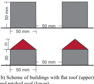
The surface is covered by series of identical and paral-lel street canyons (Figure 1b). The area of the interest lies as far as possible from the channel entrance to provide a long fetch for development of a fully turbulent boundary layer ([9]) and at the same time it far enough from the end-ing part of the wind-channel. Two geometries of roof are tested - triangle and flat. The model streets have 50 mm in dimension when using scale 1:400.

The ratio of the frontal area of model with respect to the cross-section of channel is 20%. This causes an unde-sirable aerodynamical blocking of the approach flow due to developing of an internal boundary layer. Therefore, the results of measurement can be hardly applicable on the real

250 mm

Z

X

Measuring area Y

50

50

////

50

2 000 mm

3000 mm

////

Laser

(a) Scheme of model of street canyons inside the channel. Flow is coming from the left side. Green area denotes the sheet light of laser for PIV.

20

50 mm

50

mm

50 mm

30 _{50 mm}

50 mm

(b) Scheme of buildings with flat roof (upper) and pitched roof (lower)

Fig. 1: Scheme of the experimental set-up.

conditions. Nevertheless, dynamics of lower layer up to ap-proximately Z/H=1.5 match well with a boundary layer in a wind-tunnel, where the layer is modeled properly ([8]). Above this level, the higher is the elevation, the more devi-ation from the correct boundary layer appears.

Particle Image Velocimetry (PIV) with a relatively high repetition rate (500 Hz) is used to measure instantaneous velocity values in the vertical plane. Flow is filled by oily tracer particle with mean radius of approximately 1 μm. One run of PIV measurement consists of 1600 snapshots, each of them with 4800 velocity vectors. The spatial reso-lution result to 1.2 mm x 1.2 mm thanks to the overlapping of 50%. The acquisition time is 3.2 s. In the table 1, the parameters of PIV set-up are published.

Table 1: Diode pumped Nd:YLF laser.

Repetition rate 500 Hz

Repetition rate 1280×1024 pxs

Interrogation area 32×32 pxs

Overlapping 50% (80×64 vectors)

Energy 10 mJ

Area 100×100 mm

Acquisition time 3.2 s

2.1 Wavelet analysis

temperature or a concentration (for example [10], [11]. The basic principle of Wavelet transformation is to convolute a signal and a so-calledmother waveletfunction. The mother wavelet might be an arbitrary function as well as far it ful-fills the criterion of admissibility. Admissibility condition means that the function quickly falls to zero with f → ±∞ and it has a zero mean value. Thedaughterfunction is in-ferred from the mother one by a dilation (i.e. change of the frequency and change of the length of a support of the function) and by a translation over the time.

We have applied two often used mother functions, ”Mex-ican hat” and ”Morlet function”. Mathematical definitions of these functions are written in the table 2.

Table 2: Wavelet mother function

Mexican hat ψ(t)=(1−t2_)et2/2

Morlet ψ(t)=π−1/4_ei2πf0t_e−t2/2

The Mexican hat is popular for its good sensitivity to ’see’ the ramp-like or saw-tooth pattern, so-called isolated sharp step change of the signal ([12], [13]). These patterns were detected in velocity or scalar time-series measured in-situ above a plant canopy like a forrest, an orchard or a cereal field.

Morlet function is more suitable for detection of a sinu-soidal pattern in the signal. It has also a simpler image in the Fourier space what results in better localization of the frequency. The angular velocity in this paper is chosen to beω0=6 and frequencyf0=0.9549.

The convolution between the signal and daughter func-tion is namedwavelet coefficient. When the spectrum al-gorithm employs the velocity fluctuations, the square of the modulus of the wavelet coefficient represents turbulent kinetic energy. In this study, themodulusand the power, the square of the modulus, both divided by the acquisition time, were evaluated.

For calculation itself, we basically adopted Matlab code developed by [14]. Small modification according the rec-ommendation of [15] was made and then, we applied a proper normalization. Some preliminary results from the Wavelet analysis applied to data from the street canyon are published in [16].

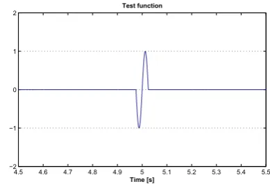
We have tested both mother functions and compared their results. In Figure 2 is seen the original signal, a sim-ple one wave with frequency of 20 Hz. Figure 3a depicts transformation into local power spectra by Morlet func-tion, whereas Figure 3b displays the Wavelet transforma-tion with Mexican hat functransforma-tion. The graph of the local power spectra is calledscalogram. On the abscissa is plot-ted time in seconds, on the ordinate axis is plotplot-ted fre-quency in Herz and the color of wavelet coefficient follows the turbulent kinetic energy.

The Morlet power pattern is apparently compact, better defined in frequency than the one derived from the Mexi-can hat function. MexiMexi-can hat shows separated spots with gap in between. The time-location of the gap precisely cor-responds to the time when test wave crosses the zero level. The temporal resolution of Mexican hat is therefore better than in the Morlet case. Notwithstanding, the magnitudes

4.5 4.6 4.7 4.8 4.9 5 5.1 5.2 5.3 5.4 5.5

−2 −1 0 1 2

Time [s] Test function

Fig. 2: Test function - simple wave with frequency of 20 Hz.

Time [s]

Frequency [Hz]

Morlet wavelet transform of sinusoidal wave

4.5 4.6 4.7 4.8 4.9 5 5.1 5.2 5.3 5.4 5.5 64

32 16 8 4 2

0 0.05 0.1 0.15 0.2 0.25 0.3 0.35 0.4 0.45 0.5

(a) Wavelet analysis with Morlet fucntion as a mother wavelet.

Mexican hat wavelet transform of sinusoidal wave

Time [s]

Frequency [Hz]

4.5 4.6 4.7 4.8 4.9 5 5.1 5.2 5.3 5.4 5.5

64 32 16 8 4 2

(b) Wavelet analysis with Mexican hat as a mother wavelet.

Fig. 3: Wavelet analysis of the test function.

of power reach the same values for both functions. Further-more, the total spectral characteristics collapse into each other (not shown).

Regarding the physical interpretation of the scalograms, we usually obtain frequency and time information of a highly energetic event, therefore one could get an understanding about particularly important frequencies appearing in the flow and the time of their emergence and cessation - and the duration of the events.

interpret the physical meaning of the scalograms spots through coupling of the certain spots with clear physical dynamics in the velocity field.

3 Results

3.1 Detection of the events

When applying Wavelet analysis on the longitudinal and the vertical velocity component in the region of the inten-sive turbulence, the results are strikingly similar to each other (see Figure 4a and Figure 4b). In both the longitudi-nal and vertical case, the strongest patterns collapse into the same times and the frequencies. It witnesses about a high correlation between longitudinal u’ and vertical w’ ve-locity fluctuation. This is not surprising since it is known that the momentum flux<−uw>is enhanced in the tur-bulent boundary layer (BL).

Within a street canyon, the flux reaches the maximum value approximately at the roof-top level ([17], [18]). When decomposing the momentum fluxes according to the Quad-rant analysis, the major contributor to the< uw > mo-mentum flux becomes a sweep and an ejection, especially inside the shear layer generated by the roof ([19]). Further, according to [19], the very dominant events in terms of instantaneous momentum flux distributed spatially in the street canyon are again the sweep and the ejection. They both supply a large portion of momentum flux occurring at given times. It was revealed the sweep and the ejection can represent up to 80%-90% of total momentum flux in the canyon cross-section (plane XZ).

The sweep and the ejection also accompany many of the organized structures in the turbulent flow. If we subtract a convective velocity of the vortex core from the whole flow ([4]), the vortex then reveals its natural circular shape. On the downstream part of the vortex lies sweep area, on the rear part, ejection area appears. The same can be draft for wavy patterns passing in the flow. The downward part of the wave is represented very often by the sweep and the upward part by the ejection. Very rarely is the downward part represented by the inward interaction and upward part by the outward interaction, however this can occur in the flow as well.

To get a certain insight into the interesting flow events, we studied the 3.2 s lasting video from PIV. The video is recorded with 500 Hz sampling frequency, so 1600 snap-shots of velocity vectors with temporal steps of 0.002 s shows the dynamics in the street canyon. The video shows several propagations of the air into the canyon (sweep) and escape of the air from the canyon (ejection), many small vortical structures generated on the roof-top level, waves going above the roof-top level with acceleration and decel-eration.

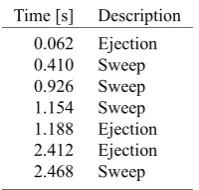
We will focus on activities when the flow regime in the canyon is influenced the most. These are strong sweep and ejection event. The overview of some them are listed in the table 3.

We picked up two significant occasions, which should be captured by whatever analysis, since they were appar-ently the most dominant processes in the whole period. The first is the strong sweep event at T=0.410 s and second

is the extreme outflow-ejection events at T=2.412 s. Then, we tested various Wavelet analytical approaches whether they are capable to detect these two events precisely and unambiguously.

Table 3: Significant sweep-ejection in the flow.

Time [s] Description

0.062 Ejection

0.410 Sweep

0.926 Sweep

1.154 Sweep

1.188 Ejection

2.412 Ejection

2.468 Sweep

3.2 Wavelet analysis of the longitudinal and the vertical velocity

Firstly, we conducted analysis on the longitudinal veloc-ity U. We picked up a representative spatial point in the middle of the canyon at the roof top level. The point has coordinates X/H=0 and Z/H=1, where H is height of the building. This is the point that would probably be chosen by many researchers, since it is simply well-defined point in any street canyon.

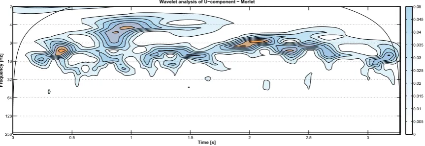
Morlet wavelet function convoluted with velocity U carries out the scalogram in Figure 4a. The square of modu-lus of complex wavelet coefficient brings number of highly energetic spots between 8 and 16 Hz, and some of around 4 Hz. Only a very few events, or events with low energy hap-pen with frequencies higher than 16 Hz. The tested sweep and ejection events are apparently visible but one big prob-lem arouse. The sweep and ejection are not distinguishable from each other. They also are not discernible from all the other events occurring during 3.2 s of recording. This is inconvenient and it yields the necessity to find another ap-proach that can identify the events better.

When implementing Mexican hat, the square of mod-ulus is rather confusing, since it carries out an enormous number of the spots. The energy, frequency and timing of the spots are in agreement with spots in Morlet case. Notwithstanding, the number of patches is so high that the whole picture becomes almost unreadable.

Time [s]

Frequency [Hz]

Wavelet analysis of U−component − Morlet

0 0.5 1 1.5 2 2.5 3

256 128 64 32 16 8 4 2

0 0.005 0.01 0.015 0.02 0.025 0.03 0.035 0.04 0.045 0.05

(a) Square of modulus of wavelet coefficient of the longitudinal velocity U.

Time [s]

Frequency [Hz]

Wavelet analysis of W−component − Morlet

0 0.5 1 1.5 2 2.5 3

256 128 64 32 16 8 4 2

0 0.005 0.01 0.015 0.02 0.025 0.03 0.035 0.04 0.045 0.05

(b) Square of modulus of wavelet coefficient of the vertical velocity W.

Fig. 4: Wavelet analysis with Morlet as a mother wavelet function applied to velocity time-series from point X/H=0, Z/H=1.

Two big events are visible at time T=0.410 s and T=0.926 s. The first one matches to the searched special event. The second one is one of the events from the table 3.

Unfortunately, the ejection event in the later part of sig-nal T=2.412 s is not visible enough, the method did not see this strong ejection properly. The scalogram in Figure 5b of the vertical component exhibits apparently the ejection (orange color) but on contrary, it detected the sweep event very mildly.

3.3 Wavelet analysis of the momentum flux

The information about acceleration and deceleration of the flow in the horizontal and the vertical direction is interest-ing but insufficient for reliable detection of the organized motion. Thus we attempted to analyze momentum flux it-self. Figure 6a depicts the time-series of momentum flux in the before-mentioned point (X/H=0, Z/H=1). We also chose a certain threshold (red solid line). The threshold can be arbitrary number suitable for the intensity of the event we are looking for. The lower intensity, the lower threshold has to be chosen and the more events (even undesired) can be detected. In our case the threshold equals to value of -4 what results in 19 detected events. After inspection of the

PIV video, most of the strong events belongs to the sweep group.

We applied Mexican hat function solely to this time-series, since the shape of enhanced momentum flux fits well with the shape of Mexican hat (Figure 6b). The strong sweep activity occurring at time T=0.410 s is detected well. Some of the other events are detected too, however the ejec-tion almost vanished from the scalogram. There is only a large spot with very low energy in low frequencies. Since the ejection lasts for long time (i.e. it has long period), the low frequency would be correct. This ejection contains low momentum flux, so it can hide itself the natural variance of the momentum flux. The ejection even does not exceeds the threshold and it does not convolute with Mexican hat function so the final wavelet coefficient is weak.

3.4 Wavelet analysis of theδ−S

Since the previous approaches provided only limited re-sults or were not able to detect both of the significant events, we have changed the approach. We posed two questions:

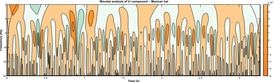
Wavelet analysis of U−component − Mexican hat

Time [s]

Frequency [Hz]

0 0.5 1 1.5 2 2.5 3

64 32 16 8 4 2

−5 −4 −3 −2 −1 0 1 2 3 4 5 x 10−3

(a) Modulus of wavelet coefficient of the longitudinal velocity U.

Wavelet analysis of W−component − Mexican hat

Time [s]

F

requency

[H

z

]

0 0.5 1 1.5 2 2.5 3

64 32 16 8 4 2

−5 −4 −3 −2 −1 0 1 2 3 4 5 x 10

(b) Modulus of wavelet coefficient of the vertical velocity W.

Fig. 5: Wavelet analysis with Mexican hat as a mother wavelet function applied to velocity time-series from point X/H=0, Z/H=1.

2 Where in the street canyon is the spatial point which is the most representative for processes happening in the whole street canyon?

To answer the first question, we have focused more on momentum flux contained only in the sweep and the ejec-tion itself. Each time-series of the momentum flux can be decomposed by Quadrant analysis into four quadrants ([8, 20]). The time-series of either the sweep or the ejection can be extracted. We could combine this time-series together by inserting this selected data into empty data-series. It is convenient to preserve the sign of the sweep (naturally neg-ative) and inverse the sign of the ejection momentum flux (changed from naturally negative to positive) and both in-sert into one time-series.

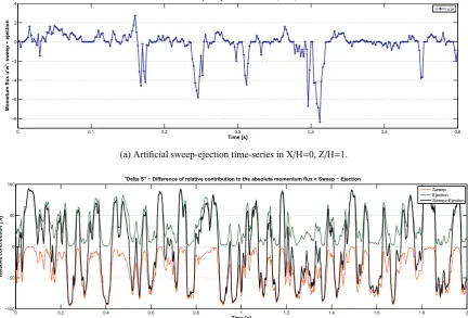
At each instant of time, momentum flux can belong only to one of four quadrants. If we insert sweep and ejec-tion, the rest of the time is not covered by these two quad-rants and it is filled by zeroes. As was shown in [19], the sweep and the ejection together occupy almost 80% of the acquisition time period, so only 20% of signal is empty. The example of the artificial time series from point X/H=0, Z/H=1 is in Figure 7a. It is clear that large majority of the signal is covered. It can be also deduced that the momen-tum flux in absolute sense contained in the ejections (posi-tive values) is lower than in the sweeps (nega(posi-tive values).

Second question needs a further preparation. As we mentioned in the section 3.1, from the spatial point of view, the relative contribution of the sweep momentum flux

cap-tured in frozen picture of the street canyon might be 80%. The same stays for the ejection. This maximum relative contributions are attained from time to time. Also, they pass the canyon in alternative fashion, so the sweep peaks are almost regularly altered by the ejection peaks and so on. There are also time intervals, when sweep contribution decreases in favor of the ejection and vice versa. At the mo-ments when relative contribution from one event becomes lower than relative contribution from second event, these relative contribution usually gains typical value of 40%. In other words, if we determine a threshold of 40%, momen-tum flux in street canyon is exclusively absorbed in either the sweep or the ejection. This is process happening inte-grally in the whole XZ cross-section of the canyon, thus we need to find an one-point location that is perfectly (or as much as possible) representative for processes inside the whole area.

The idea is to compare data-series from many locations with one time-series that suitably represents the overall pro-cesses in the canyon. The relative contribution of the sweep and the ejection seems to be suitable such date-series. Only problem is how to create a proper time-series similar to one in Figure 7a, since at given time instants, there is momen-tum flux coming from both the sweep and the ejection.

0 0.5 1 1.5 2 2.5 3 −12

−10 −8 −6 −4 −2 0 2

Time [s]

u’w’

u’w’ (X/H=0, Z/H=1)

u’w’

Ejection

Sweep

(a) Time-series of u’w’ with threshold.

Wavelet analysis of u’w’ − Mexican hat

Time [s]

Frequency [Hz]

0 0.5 1 1.5 2 2.5 3

256 128 64 32 16 8 4 2

0 0.005 0.01 0.015 0.02 0.025 0.03 0.035 0.04 0.045 0.05

(b) Wavelet analysis of time-series u’w’.

Fig. 6: Time-series of ’u’w’ at point X/H=0, Z/H=1 (a) and its Wavelet analysis using Mexican hat (b).

error into the time-series of sweep and ejection notwith-standing due to a certain exclusivity above threshold, the data were only slightly modified. The time-series with the sweep (red thin line) and the ejection (green thin line) rel-ative contribution and final data-series (black thick line) is depicted in Figure 7b.

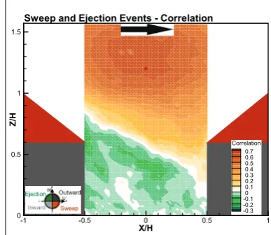
Comparison between one-point data and representative data-series is made by the correlation. Figure 8 shows, how much correlated are various spatial locations to the repre-sentative series. We can see that high correlations (C=0.7) occur in a large elliptic region above the roof-top level. The region extends vertically from Z/H=1.15 up to Z/H=1.5 and horizontally from X/H=-0.3 to X/H=0.2.

We could say that all above roof area is highly corre-lated with sweep-ejection processes. This is in agreement with the conclusion in [19], the majority (almost 90%) of the sweep and ejection happens above the roof.

The level of the correlation decreases downward. Cor-relations even attain small negative values (C=-0.3) at the bottom of the street. This anti-correlation is weak, however it can suggest that while the sweep is coming into upper part of canyon, the ejection occurs at the bottom and vice versa.

We pinpointed the dot in the highly correlated area a red dot (coordinates X/H=0, Z/H=1.2) and executed here Wavelet analyzes. The position can be taken wherever in-side the elliptical area and there will no be significant diff er-ence in precision. The final scalogram with modulus based on Mexican hat convolution with the sweep-ejection time-series is in Figure 9.

X/H

Z/H

-1 -0.5 0 0.5 1

0 0.5 1 1.5

Correlation 0.7 0.6 0.5 0.4 0.3 0.2 0.1 0 -0.1 -0.2 -0.3

Sweep and Ejection Events - Correlation

Fig. 8: Correlation between time-series created by insert-ing sweep (with true negative sign) and ejection (with pos-itive sign) in all points in the canyon and from time-series Figure 7b.

0 0.1 0.2 0.3 0.4 0.5 0.6 −8

−6 −4 −2 0 2 4

Time [s]

Mometum flux u’w’: sweep − ejection

Extracted sweep and ejection momentum flux, X/H=0, Z/H=1

u’w’

(a) Artificial sweep-ejection time-series in X/H=0, Z/H=1.

0 0.2 0.4 0.6 0.8 1 1.2 1.4 1.6 1.8 2

−100 −50 0 50

100 "Delta S" − Difference of relative contribution to the absolute momentum flux = Sweep − Ejection

Time [s]

Relative contribution [%]

Sweep Ejection Sweep−Ejection

(b) Artificial sweep-ejection relative contribution to the total momentum flux in the canyon. Sweep is negative, ejection is positive.

Fig. 7: Artificial time-series created by inserting sweep with true negative sign and ejection with inverse sign (now positive).

Wavelet analysis of Delta S − Mexican Hat

Time [s]

Frequency [Hz]

0 0.5 1 1.5 2 2.5 3

64 32 16 8 4 2

−5 −4 −3 −2 −1 0 1 2 3 4 5 x 10−3

(a) Modulus of wavelet coefficient applied to artificial sweep-ejection time-series.

Fig. 9: Wavelet analysis with Mexican hat as a mother wavelet function applied to artificial sweep-ejection time-series in point X/H=0, Z/H=1.2.

numerically modeled) longitudinal and vertical component of velocity.

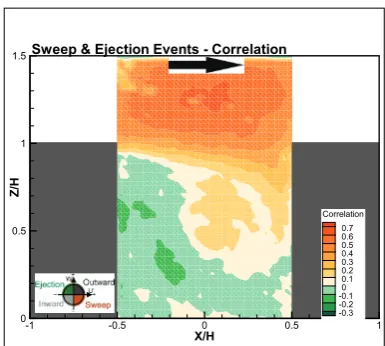
The very similar results were gotten from the flat roof case. The correlation between one-point time-series and ar-tificial sweep-ejection carries out the same highly-correlated area above the roof-top of the canyon building (see Fig-ure 10). This is actually very advantageous locality to an-alyze since the middle of the canyon and region between

X/H

Z/H

-1 -0.5 0 0.5 1

0 0.5 1 1.5

Correlation 0.7 0.6 0.5 0.4 0.3 0.2 0.1 0 -0.1 -0.2 -0.3

Sweep & Ejection Events - Correlation

Fig. 10: Correlation between time-series created by insert-ing sweep (with true sign) and ejection (with inverse sign) in all points in the canyon from and time-series Figure 7b.

4 Conclusions

The paper describes the way how to detect a certain orga-nized structures in the flow inside the street canyon. The main intention was to search sweep and ejection events. The Wavelet analysis is used for detection of highly en-ergetic sweep-ejection process. Two mother wavelet func-tions were implemented, each turned out to be suitable for identification of different structures.

The best results were obtained with modulus of Mexi-can hat. Modulus brings the benefits of information about the sign (or direction of change) of the physical quantity. The best quantity for analysis turns out to be the sweep-ejection artificial time-series that can be easily calculated from every 2-component velocity measurement. There is a location where one-point data-series are highly correlated with behavior of the whole canyon. Such time-series, taken in these recommended points, reliably describes the inte-gral behavior of the flow inside the canyon and can be suc-cessfully used for Wavelet analysis.

Acknowledgement

The authors kindly thank the Czech Science Foundation (project

GAP101/12/1554) for financing this project.

References

1. J. Zhou, R.J. Adrian, S. Balachandar, T. Kendall, J. Fluid

Mech.387, 353 (1998)

2. S. Leonardi, P. Orlandi, L. Djenidi, R. Antonia, International

Journal of Heat and Fluid Flow25, 384 (2004)

3. O. Coceal, A. Dobre, T.G. Thomas, S.E. Belcher, J. Fluid

Mechanics589, Cambridge University Press (2007)

4. R.J. Adrian, C.D. Meinhart, C.D. Tomkins, Journal of Fluid

Mechanics422, Cambridge University Press (2000)

5. C.D. Tomkins, R.J. Adrian, J. Fluid Mech.490, Cambridge

University Press (2003)

6. S.K. Robinson, Annual Review of Fluid Mechanics23, 601

(1991)

7. Z.C. Huang, H.H. Hwung, K.A. Chang, Coastal Engineering

57, 795 (2010)

8. R. Kellnerova, L. Kukacka, K. Jurcakova, V. Uruba,

Z. Janour, Journal of Wind Engineering and Industrial

Aero-dynamics104-106, 302 (2012)

9. H. Cheng, I.P. Castro, Boundary-Layer Meteorol.105, 411

(2002)

10. W. Gao, R.H. Shaw, K.T. Paw U, Boundary Layer

Meteorol-ogy47, 349 (1989)

11. R.H. Shaw, J.J. Finnigan,Eddy Structure Near Plant Canopy

Interface, in17th Symposium on Boundary Layers and

Tur-bulence, Conference proceeding(San Diego, Canada, 2006),

p. p. J2.1

12. W. Gao, B.L. Li, J. Appl. Meteor.32, 1717 (1993)

13. J. Qiu, K. Paw U, R. Shaw, Boundary-Layer Meteorology72,

177 (1995)

14. C. Torrence, G.P. Compo, Bull. Am. Meteorol. Soc.79, 61

(1998)

15. Z. Ge, Annales Geophysicae25, 2259 (2007)

16. R. Kellnerova, L. Kukacka, J. Odin, V. Uruba, P.

An-tos, Z. Janour,Comparison of Wavelet analyses applied to

very rough boundary layer data, inProceedings of

Czech-Japanese Seminar in Applied Mathematics, edited by S.Y.

Michal Benes, Masato Kimura (Institute of Mathematics for

Industry, Kyushu University, 2010), Vol. 36 ofCOE Lecture

Note, pp. 36–45

17. P. Kastner-Klein, M.W. Rotach, Boundary-Layer Meteorol.

111, 55 (2004)

18. R. Kellnerova, L. Kukacka, Z. Janour, Acta Technica CSAV

54, 401 (2009)

19. R. Kellnerova, V. Fuka, L. Kukacka, V. Uruba, Z. Janour,On

the quadrant analysis of the flow in the street canyon, inEPJ

Web of Conferences(2013), Vol. 45,www.scopus.com

20. L. Kukacka, S. Nosek, R. Kellnerova, K. Jurcakova,