A Bayesian Monte-Carlo Uncertainty Model for Assessment of Shear Stress Entropy

(1)

A Bayesian Monte-Carlo Uncertainty Model for Assessment of Shear Stress

Entropy

Amin Kazemian-Kale-Kale a, Azadeh Gholami a, Mohammad Rezaie-Balf b, Amir Mosavi c,d*, Ahmed A Sattar e, Bahram Gharabaghi f, Hossein Bonakdari g**

a _{Environmental Research Centre, Razi University, Kermanshah, Iran}

b _{Department of Water Engineering, Graduate University of Advanced Technology, Kerman,}

Iran

c _{Kalman Kando Faculty of Electrical Engineering, Obuda University, Budapest, Hungary;} [email protected]

d _{Institute of Structural Mechanics, Bauhaus University Weimar, D-99423 Weimar, Germany;}

[email protected]

e _{Department of Irrigation & Hydraulics, Faculty of Engineering, Cairo University, Giza,}

German University in Cairo, Egypt

f _{School of Engineering, University of Guelph, Guelph, Ontario, NIG 2W1, Canada}

g _{Department of Soils and Agri‐Food Engineering, Laval University, Québec, Canada, G1V0A6;}

[email protected]

(2)

Abstract: The entropy models have been recently adopted in many studies to evaluate the

distribution of the shear stress in circular channels. However, the uncertainty in their predictions and their reliability remains an open question. We present a novel method to evaluate the

uncertainty of four popular entropy models, including Shannon, Shannon-Power Low (PL), Tsallis, and Renyi, in shear stress estimation in circular channels. The Bayesian Monte-Carlo (BMC) uncertainty method is simplified considering a 95% Confidence Bound (CB). We developed a new statistic index called as FREEopt-based OCB (FOCB) using the statistical

indices Forecasting Range of Error Estimation (FREE) and the percentage of observed data in the CB (Nin), which integrates their combined effect. The Shannon and Shannon PL entropies

had close values of the FOCB equal to 8.781 and 9.808, respectively, had the highest certainty in the calculation of shear stress values in circular channels followed by traditional uniform flow shear stress and Tsallis models with close values of 14.491 and 14.895, respectively. However, Renyi entropy with much higher values of FOCB equal to 57.726 has less certainty in the

estimation of shear stress than other models. Using the presented results in this study, the amount of confidence in entropy methods in the calculation of shear stress to design and implement different types of open channels and their stability is determined.

Keywords: Shear stress distribution, entropy, uncertainty, Shannon, Shannon PL, Tsallis, Renyi

1. Introduction

(3)

many places within urban sanitary or storm sewer networks, the flow tends to slow down, allowing carried sediment to be deposited on channel bed. With time and continuous deposition of sediment, the circular bed shape tends to build up in the form of irregular or flatbeds. This leads to the change in the channel shape, which alters the hydraulic characteristics of flow and shear distribution in the channel. This process is often encountered in practice, and many circular channels exhibit flatbeds. In circular open channels, the shear stress distribution has been

experimentally analyzed by many researchers [ 31 ]. Others have developed models to predict the -distribution of shear stress along a channel using numerical and analytical methods [4-6].

Numerical models depending on soft computing (SC) techniques have been recently presented for the prediction of shear stress distribution [7,8].

The entropy concept has been used by researchers to predict different flow variables such as velocity distribution [9-11], transverse slope of stable channels banks [12-14], and shear stress distribution [15]. Chiu [16], for the first time, introduced models for calcualting the shear stress in open channels using the Shannon entropy concept. Sterling and Knight [17] developed equations based on Shannon entropy for estimating boundary shear stress in open channels. Although, their results showed this approach could estimate the distribution of the shear stress reasonably well, however, they indicated some practical limitations in application of the Shannon entropy for practical cases. Sheikh and Bonakdari [18] employed the entropy concept and

(4)

Other entropies such as Tsallis and Renyi concepts can be applied to measure the probability of variables [14,19]. Tsallis [20] proposed Tsallis entropy as a generalization of the Shannon

entropy comprising a supplementary parameter. Renyi and Tsallis entropies with non-additive parameters can be utilized to perform it less susceptible to the form of the probability distribution [14, 21-23]. Bonakdari et al. [24] showed that the Tsallis method could calculate the shear stress distribution along the wetted perimeter with reasonable accuracy. Khozani and Bonakdari [25] employed the Renyi entropy and presented a relationship for estimation of the shear stress

distribution in circular channels. They concluded that their presented model showed the ability to calculate the shear stress distribution and compared well to measured results. Although many studies carried out on entropy models for prediction of shear stress distribution, wide

implementation of entropy models has not taken place due to the absence of enough confidence in these models compared to previous conventional models in estimation of flow variables. Thus, it is beneficial to analyze the uncertainty of entropy models and compare the performance of them with previous conventional models.

The uncertainty analysis of many hydraulic and hydrological models has been tackled by many researchers using various uncertainty methods [26-40]. Lamb et al. [41] used measured water depth in a Bayesian procedure as Generalized Likelihood Uncertainty Estimation (GLUE) to measure uncertainties for a simple model of the rainfall-runoff distribution. Misirli et al. [36] used the Bayesian Recursive Estimation (BaRE) to evaluate the watershed model’s uncertainty. They introduced the FREE statistic index for evaluating models’ uncertainty. FREE is equal to the absolute sum of the measured data within the confidence bound (FP) and the absolute sum of

the measured data outside the confidence bound (FN). Thus, the FREE index represents the width

(5)

analyzed the uncertainty of the Shannon entropy model in estimating the velocity distribution proposed by Moramarco et al. [43]. The proposed model for estimating velocity in their study was satisfactory for calculating the average velocity in multiple segments with 95% CB, but they did not present any results for the model's ability to calculate the velocity distribution at the channel cross-section. Rincon [44] provided a comprehensive overview of uncertainty methods that are widely used in hydrodynamics. Rincon [44] concluded that BMC is a powerful method for evaluating sources of uncertainty in hydrodynamic modeling. He stated that despite the BMC calculations required, this method could be easily applied in most cases.

In the fields of measuring the uncertainty of entropy models in the estimation of shear stress distributions in open channels, based on the knowledge of authors, no study is seen except the recent studies related to authors. Kazemian-Kale-Kale et al. [45], analyzed the Tsallis entropy uncertainty in the prediction of shear stress distribution in circular channels for the first time. Their proposed uncertainty method was based on models with Gaussian (normal) error distributions. Therefore, firstly, they studied the error distribution of shear stress predicted by Tsallis entropy and they emphasized on the necessity to normalize the shear stress data for the uncertainty analyses. Then, they calibrated the model to select the best sample size (shear stress data considered under different hydraulic conditions) and finally analyzed the uncertainty of the Tsallis entropy model using this Sample Size (SS). Although their results were well capable of evaluating the uncertainty of the Tsallis model, the calibration method was difficult, and in addition, they did not discuss the performance of the different transfer functions to normalization in the uncertainty results. Kazemian-Kale-Kale et al. [46] also analyzed the uncertainty of

(6)

Shannon entropy uncertainty. Kazemian-Kale-Kale et al. [45, 46] studied the uncertainty of the Tsallis and Shannon entropy models in calculating of shear stress distribution. However, because these statistics need to be examined simultaneously to determine each model’s uncertainty, they were not able to compare the uncertainty of different entropy models. Therefore, they did not discuss the reliability of the Shannon and Tsallis entropy models in calculating shear stress compared to other models.

Based on these gaps, this paper aims at providing a novel uncertainty model for quantifying and evaluating the uncertainty of four different entropy models; Shannon, Shannon PL, Tsallis, and Renyi, in calculating shear stress in the circular channels. The obtained results are compared to those calculated by the established analytical equation for shear stress in uniform flow. The uncertainty method introduced by Kazemian-Kale-Kale et al. [46] based on the BMC method is briefly presented as the Hybrid Bayesian and Monte-Carlo Estimation System (HBMES-1) then further improved, and the uncertainty method is presented in this study as HBMES-2. Using the improved model, the uncertainty of several different entropy models and the optimized/minimum CB that covers all measured data (OCB) are defined. The improved model is based on the

optimized OCB (width of the confidence bound) and the absolute sum of measured data FREEopt.

Given the value of OCB and FREEopt, the FOCB statistic is introduced that can show the effect

of all uncertainty statistics. FOCB shows the degree of qualitative and quantitative uncertainty of shear stress models. Since the main purpose of current study is to assess and compare the

(7)

2. Material and methods

2.1. Entropy models 2.1.1. Shannon model

Sterling and Knight [17] employed Shannon entropy to present a model to predict shear stress distribution in circular channels as follow:

        − + = 2 ) 1 ( 1 ln

1 ₀_max

0 P

y e



 (1)

where τ is the local shear stress distribution, τmax is the maximum shear stress, P is the wetted

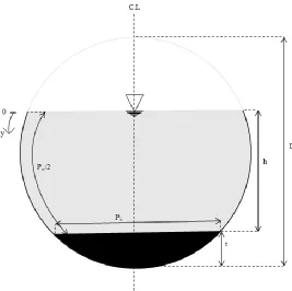
perimeter of the circular channel, and y is the specific point in wetted perimeter, which we want to obtain the shear stress on it; value changes between 0 to P/2. Figure 1 shows the circular cross-section with related notations used in models. The shear stress values are only computed for half the wetted perimeter due to section symmetry and, consequently, hydraulic

characteristics. In Equation (1) λ0 is the Lagrange multiplier that can be determined as:

1 max 0 1 1 m ax 0 m ax 0 −       − − = gRs e e _      (2)

where ρ is the fluid density, g is the gravity coefficient, R is the hydraulic radius, and s is the channel slope. In a circular channel with a flatbed, Equation (1) can be written as follows:

( )

(

)

(

)

2 2 1 1

1 0 m a x

0 w w w w w w P y y P y y

e w w  

      ₊ ₋ − =     (3) ( )

(

)

(

)

w b w b w b b y P y P P y y

e b b   +

      ₊ ₋ − = 2 2 2 1 1

1 0 m a x

0

 



(8)

where_max_{( )}_w and _max_{( )}_b , are the maximum shear stress at the wall and bed of channel respectively, Pw and Pb are the wetted perimeter corresponding to the wall and bed of the

channel, and yw is an offset and taken as 5 mm in their analysis.

The equations presented by Knight et al. [47] were used to predict the mean and maximum shear stress for wall and bed of circular with the flatbed channel as:

(

b w

)

w

w _SF _P _P

gRS =0.01% 1+

 

(5)

(

w

)(

b w

)

b _SF _P _P

gRS= 1−0.01% 1+

 

(6)

( )



₍ ₎0.7108



max 0372 . 2 % 01 .

0 _w _b _w

w P P SF gRS =   (7)

( ) ₍ ₎



₍ ₎0.3287



max 1697 . 2 % 01 . 0

1− −

= _w _b _w

b P P SF gRS   (8)

where w and b are the mean wall, and bed shear stress, respectively, and %SF is the wall

shear force percentage determined by the following equation:

(

)

(

3.23log 1 4.6052

)

exp

%SF_w =C_sf − P_b C₂P_w+ + (9)

where C2 =1.38 and Csf =1.0 for 4.374

w b

P P

, otherwise ( )0.28125

6603 .

0 _b _w

sf P P

C = .

Figure 1. Cross-section of the circular with the flatbed channel and its notation.

2.1.2. Shannon PL model

(9)

n P y 1 max ) 2 ( 

 = (10)

where n is a non-dimensional parameter computed as:

   − = max n (11)

where  is the mean shear stress value. It should be noted that these equations are used to predict the wall and bed sear stress of circular with flatbeds channel separately. The mean and maximum shear stress values are given in Equation (11) are obtained from Equations (5)-(8). In the entropy models presented below, the Equations (5)-(8) are also used.

2.1.3. Tsallis entropy model

Bonakdari et al. [24] employed the concept of Tsallis entropy to present the following relationship for estimating shear stress in a circular channel:

1 2 1 1 2 1 ) (     

 = _ k+ _ k−

P y k k (12) where q q

k= −1, q is a real value, λ1and λ2 are Lagrange multipliers that can be determined

from the two following equations:



  

k k k

k

1 2 max 1

2   

 + − = (13)

        

 _k k _k 2_kk

1 max 1 2 max 1 2 1

max( +1) [ + ] −[ + ]=( +1) (14)

2.1.4. Renyi entropy model

(10)

                            −    −  − −  −  =    k k k P y 1 max 2 ) 1 ( ) ( 1         (15) where 1 −   =   

k and αʹ is a real number between zero and one. λ′and λ″ are Lagrange

multipliers that can be calculated with two following equations [25]:

(

) ( )

       −  =   − −  −  −    1 k k k (16)

(

)



(

)

( )



₍

₎

        

 ( 1) 1 ˆ

1

1 1 1

2 ' ₋  =  − −  −  − +   −  −  − −  +  + 

 k k k

k

k (17)

where

max

ˆ  

 = is the dimensionless mean shear stress.

2.2. Global shear stress (ρgRs)

The shear stress in open channels in case of uniform flow is considered as a basic model for comparison with entropy models as follows:

gRs



 = (18)

2.3. Data Collection

(11)

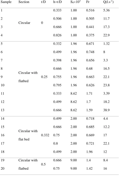
channel (t/D ≠ 0) with different bed-sediment thickness. These measured values shall be considered in the uncertainty analyses of the four entropy models.

Table 1. Summary of the hydraulic parameters in the circular channel with and without sediment.

2.4. Uncertainty analysis

The uncertainty method presented in Kazemian-Kale-Kale et al. [46] is develpoed to analyze the uncertainty of four entropy models of shear stress predictor. This method is named HBMES-1 (Hybrid Bayesian and Monte-Carlo Estimation System in the first stage). The HBMES-HBMES-1 uncertainty is improved and will be used to analyze the four entropy models in shear stress prediction. This method of uncertainty will be described further in this study as HBMES-2.

2.4.1. HBMES-1 uncertainty method

The basis of the uncertainty method presented by Kazemian-Kale-Kale et al. [45,46] was that the error distributions of the understudy models were assumed to follow a Gaussian (normal) distribution. Due to the importance of normalizing the data for the uncertainty analysis in the study of Kazemian-Kale-Kale et al. [46], two common transfer functions of Box-Cox and Johnson were compared to evaluate the shear stress estimations models’ uncertainty. Kazemian-Kale-Kale et al. [45] considered the 95% CB and performed 15 tests for uncertainty calibration based on the same CB, considering shear stress data under different hydraulic conditions.

(12)

variation of the Nin mean and the Box-Cox function transfer factor. Due to the combination of

these two statistics, the best SS based on the method of Kazemian-Kale-Kale et al. [45] will be difficult, especially when the uncertainty of several models is considered.

In this study, the best SS is selected based on the mean value of Nin. According to Corato et al.

[42], the closer Nin is to 95% CB, the assumption of the Gaussian error distribution is more

satisfying. Considering Nin’s changes, satisfy the initial condition of the Gaussian error

distribution. After selecting the best SS, the best transfer factor value is used for the final evaluation of the uncertainty. The results of this evaluation are in multiple statistics of Nin, FP,

FN, and FREE. Using these statistics, it is determined whether each of the entropy models is

sufficiently certainty to predict shear stress.

2.4.2. HBMES-2 uncertainty method

As the HBMES-1 method requires multiple statistics to be evaluated concurrently, comparing the certainty of several models using this method is very difficult and in some cases are

impossible. In this study, the HBMES-1 uncertainty method has been improved, and the result of uncertainty for each model is presented as a single statistic.

(13)

Step1. Determining initial borders of the OCB (OCBi)

First, the shear stress data are normalized using the Box-Cox transfer function and transfer factor obtained in the best SS, and then the Gaussian error distribution is calculated as follows:

) / ( ) / ( ) /

(y P =Zm y P −Zp y P

 (19)

where  (y/P) is the error of data normalization, Ze, and Zp are the normalized values of

measured and predicted shear stress (τmand τp), respectively.

Then with considering a given value for OCBi,the following relation is applied:



  

 _i

p i Z y P

P y

Z( / )|) ( / ) ( /2)

(  = +  (20)

where I = 0, 1, 2, ..., n. This value, (Z|±)i, indicates the effects of the considered OCBi and the

Gaussian error distribution (Equation 19) on the shear stress data predicted by the model. (/2)i

is the standard normal curve variable, which is related to the percentage of considered OCBi.

By performing this dividing operation;

i i OBC  = 2 100 ) ( (21)

where ψi is the area below one side of the probability distribution diagram. Using ψi from the

standard normal curve table, the value of the corresponding standard coefficient (α/2)i is

obtained. The first assumption for OCBi (OCB)0= 95%, which will be ψ0 = 0.4750 by the above

standard deviation from the table of the corresponding standard coefficient (α/2)0 =1.96. In the

Equation (20), ε and ε are the mean and standard deviation of the Gaussian error distribution of

the normalized shear stress data, respectively. Then the OCBi borders are obtained by the

Box-Cox transfer function through the following relation:

   =  + =  _  0 ] ) | ) / ( exp[( 0 ] 1 ) | ) / ( [( ) | ) / ( ( / 1      if P y Z if P y Z P y i i

(14)

where (|±)i are the borders of OCBi and λ isthe Box-Cox transfer factor.

After determining OCBi borders, the distance of the measured data from the borders (distx) and

the sum of the distances (FREE) using the equations of Kazemian-Kale-Kale et al. [46] can be calculated. If the distx value is positive, then the data is inside OCBi and if the distx is negative,

then the data is outside OCBi. As a result, the value of Nin (the percentage of measured data

within the OCBi) using distx values is obtained.

Step 2. Assessment of the final OCB (OCBn)

Given that in the OCBn, all points are within the CB, Nin should always be equal to 100%. If Nin

is equal to 100, the OCBi value is considered lower, and the three steps a-c are done. However, if

Nin is less than 100, the OCBi values considered higher, and the three steps a-c is performed. This

should continue until Nin is equal to100% and the FREE values are at their lowest value. This

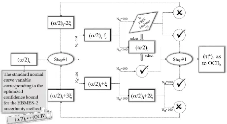
FREE value is called FREEopt. How to determine OCBn is shown in Figure 2. In this figure, ξ is

the accuracy of the standard normal table and equal to 10-2_.

Figure 2. Process of assessment of the OCBn(minimum confidence bound that covers all

measured data) in HBMES -2 uncertainty method.

Step 3. Introducing uncertainty index of FOCB

After determining OCBn, the final borders of ( n|±)n are obtained from Equation (22). In OCBn

the distx value presented in the study by Kazemian-Kale-Kale et al. [46] is optimized and derived

(15)

     − −  − − = ₋ + 0 | | ) | ( | 0 | | | ) | ( ) ( p m n m p m m n opt x if if dist         (23)

where τm and τpare the values of measured and predicted shear stress, respectively. ( |±)n

assesses the borders of OCBn, which is obtained by inserting the variable of standard normal

curve that relates to OCBn as (/2)n (Equation 22). With considering OCBn, the values of FREE

[46] are always positive, and in this paper is called FREEopt that written as follows:



 = = 0 x dist x P

opt F dist

FREE (24)

FREEopt index equals to the sum of the intervals of measured values inside the OCBn. The

OCBn and FREEopt statistics are quantitative and qualitative criterion, respectively that shall be

used to examine the uncertainty of the four shear stress predictor models. To consider the combined effect of these two statistics, the FOCB statistic is introduced such as that:

100 * _opt

n FREE

OCB

FOCB= (25)

Given that OCBn is used as a result, the present research uses the term OCB for convenience.

3. Result and discussion

Since the calibration of both the uncertainty analysis methods presented in Sections 2.4.1 and 2.4.2 are performed the same, the results of the uncertainty calibration of the four entropy models are shown first. Then, the results of the HBMES-1 uncertainty performed at the CB = 95% and the HBMES-2 results obtained with OCB are presented.

(16)

As mentioned, the calibration was done based on Nin changes to select the best SS. 15 tests

were performed for calibration, and the difference in each test varied in the number of data considered under hydraulic conditions. To select the best SS in each model, Nin values of each

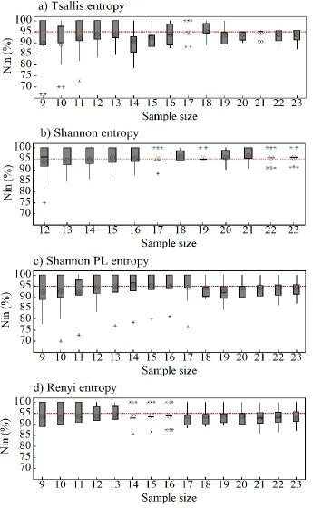
test (SS = 9 to SS = 23) were obtained at the calibration step with a default CB of 95%. Figure 3 illustrates the changes in Nin values as a box plot for all four entropy models. As stated before,

each SS that has an average Nin value is closer to 95%, is selected as the best SS. As seen in the

figure, for the Shannon, Shannon PL, Tsallis, and Renyi entropies, the closest Nin values to the

dotted line (95%) are 94.85%, 95%, 94.79%, and 94.23%, respectively. These values occur in SS amounts of 17, 15, 18, and 13, respectively. Therefore, the obtained SS values for each entropy model based on Ninvalues can be introduced as the best SS values in the calibration phase. After

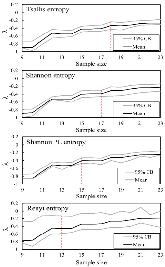
selecting the best SS, the value of Box-Cox transfer factor (λ) in this SS is considered for the final evaluation of the uncertainty of each model. So, the values of transfer factor (λ) are calculated for all models in different values of SS. These values of the λ include the average, upper, and lower limits for each SS (according to Figure 4). As seen in Figure 4, CB changes in all models are not more significant than the mean values of the λ. Thus, the mean amount of the λ

in the best SS (which is chosen based on Nin values) is selected as the best λ. According to this

figure, all model trends are similar and ascending. Changes of CB and also λ values in the initial values of SS are high, and with increasing SS value, the λ values decrease. The value of the λ in the optimized SS in the previous section (Figure 3) is determined as the best transfer factor (λ).

Figure 3. The changes in the percentage of measured values within the confidence bound (Nin)

(17)

According to Figure 4, for all entropy models, after reaching the best SS value, the variation in the λ is very low and tends to become constant. The constant changes of thefactor λ (zero

change) after the best SS indicates that in order to achieve a Gaussian error distribution in the shear stress data series, the minimum test for each model is in the best SS value. Moreover, the notable point is the similar trend in λ graphs and its change in three entropies of Tsallis,

Shannon, and Shannon PL model, unlike the Renyi entropy model. Unlike others, in Renyi entropy, the CB variations are so significant in all SS values. Therefore, the less reliability of Renyi entropy is evidence and clear in here.

Figure 4. Changes of transfer factor (λ) values in different sample sizes for all entropy models.

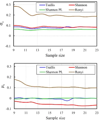
The validity of the uncertainty analysis results depends on the normality of the error distribution of each entropy model. The mean and standard deviation of the Gaussian error distribution ( and ) are also examined in the calibration stage along with the selection of the best SS. Hence, the changes of λ were obtained for various SS values  and  were calculated for different SS (sample size) values. Using the statistic, the degree of compliance of the shear stress error distribution obtained from each entropy is determined from the Gaussian distribution. The closer the error distribution is to the Gaussian distribution, leads to the greater the validity of the uncertainty results.

(18)

error distribution of the transferred data will follow Gaussian distribution. Therefore, due to the small values of for the error distribution of the shear stress obtained from the Shannon,

Shannon PL, and Tsallis, compared to the Renyi entropy, it can be said that the error distribution of these three models compared to the Renyi model are closer to the Gaussian distribution. Also, the Renyi entropy with the ε value of three times larger than those of others did not have a

favorable outcome.

The variation of the value is derived from all four entropy models, as illustrated in Figure 6. As shown in this figure, the changes of  for the Renyi entropy model is higher than those of the Shannon, Shannon PL, and Tsallis models. The values for all four models in the different SS have an almost constant value, but because the range of  variations for Renyi entropy is much higher than other models so that this value of  is less reliable in this model. The absolute values of average  for Shannon PL, Tsallis, Shannon, and Renyi models are 0.001, 0.003, 0.055, and 0.114, respectively. Therefore, the two entropies of Shannon PL and Tsallis contain less error than the Shannon entropy, and these three entropies perform better than Renyi entropy.

Figure 5. The mean and standard deviation of the Gaussian error distribution;  and , respectively; versus sample size in all entropy models.

3.2. Assessment of uncertainty of four entropy models using the HBMES-1 method

(19)

predictor model is highly reliable if 80-100% of the values are in the desired CB and the model was not able to predict if less than 50% of the values are within the CB [30,32,49,50].

Because of these studies, given the percentages of measured shear stress data within the CB equal to 95% (Nin), it can generally be said whether the entropy models are sufficiently accurate

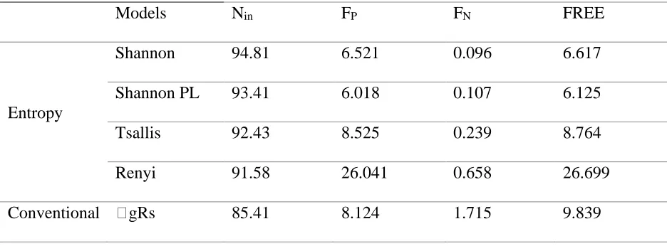
in estimating shear stress or not?. The values of Nin in column 2 of Table 2 represent the required

certainty for all models in estimating shear stress since the Nin value for all models is greater than

85%. Nin values in all entropy models are very close together and higher than Nin values for the

conventional ρgRs model.

Although Nin values can be used for certainty, to compare each model with another, FP, FN, and

FREE values should be considered in addition to Nin values. The FP values given in the third

column of Table 2 represent the absolute sum of the internal data from the borders of CB. The FN

values given in the fourth column of Table 2 represent the absolute sum of the outer data from the borders of CB. The FREE values, which are equal to the sum of FP and FN, represent the

Width of Confidence Bound (WCB) in the last column of Table 2.

The lower these FREE, FP, and FN values, means the higher model’s certainty. These three

values are close for the two Shannon and Shannon PL entropies as well as for the two Tsallis and

ρgRs models, but these values are much higher for the Renyi entropy than the other four models. As can be seen, the Nin values with the values of the three FP, FN, and FREE statistics give

different results in providing the uncertainty, and it is difficult to give a precise view to compare the accuracy of the models. For example, although the Nin value for the Renyi entropy is more

than ρgRs, the FP, FN and FREE values are much better (lower) for the ρgRs model.

Therefore, the general conclusion from the values in this table is that given the high values of

(20)

comparison of this uncertainty with respect to other statistics to be considered concurrently is complicated. In this study, HBMES-2 method is presented to solve this problem. In the next section, the results are provided and discussed in details.

Table 2. Statistical indexes based on HBMES-1 uncertainty method in shear stress prediction by different entropy models and conventional ρgRs model.

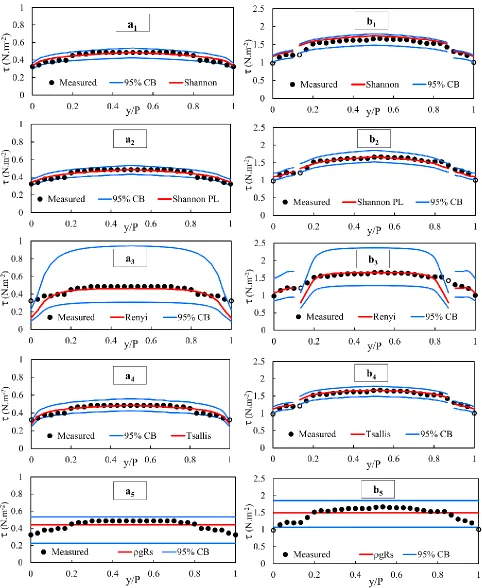
To clarify the results presented in Table 2, the shear stress distribution and 95% CB using the HBMES-1 method for a height ratio of the circular channel (t/D=0, h+t/D=0.333) and the height ratio of the circular channel with flatbed (t/D=0.25, h+t/D=0.333) is shown in Figure 6. It is seen in the figure that the trend of shear stress distribution in all four entropy models is in line with the trend of measured values for the bed area and the channel walls, whereas the conventional

ρgRs model has both a constant amount in the bed and the walls of the channel.

In the circular channel (Figure 6a), the entropy models of Shannon, Shannon PL, and Tsallis have predicted the shear stress distribution quite in accordance with the measured data. The Renyi entropy is also in good agreement with measured data except for channel sides (0<y/P<0.1 and 0.9<y/P<1). However, the performance of the Renyi entropy is much better than the ρgRs. The ρgRs model at the walls of the circular channel predicts the shear stress value much lower than the measured values, and at the bed area (0.1<y/P<0.9), it predicts the shear stress value slightly below the corresponding measured values.

(21)

However, the Shannon PL entropy, which is in accordance with the measured trend, predicts the shear stress values more than the two Shannon and Tsallis entropies.

To check the uncertainty of the models, the WCB and the percentage of measured data within the CB (Nin) in Figures 6 should be considered. The Nin value and the WCB at these height ratios

were calculated according to the overall ability of the entropy models and considering all the 23 different hydraulic conditions in Table 1. Given that the Nin in both height ratios for all models is

more than 93%, all models are capable of estimating shear stress with high certainty. Figure 6a shows that the CB for the Shannon and Shannon PL models with all data covered is very small and almost uniform.

In the Tsallis and Renyi models, two shear stress data in free surface (y/P=0) fall outside the CB (hollow points in Figure 6), indicating that the certainty of these models in predicting shear stress at the free surface of the circular channel is less than the other wet areas. This issue is more seen by Renyi entropy model. On the other hand, the WCB of the Tsallis model is much less than the WCB of the Renyi model, which demonstrates the more reliability in addition to the accuracy of Tsallis model especially in areas near the water surface.

The WCB of the ρgRs, Shannon, and Shannon PL, covered all data, but the WCB in the ρgRs is larger than the other two models. Furthermore, the ρgRs model is not capable of estimating shear stress values; so that there is no consistency with observed values.When comparing the certainty of the ρgRs and Tsallis model, it should be noted that although the Tsallis entropy has two data at the free surface outside the CB, the WCB is much lower in the Tsallis model than the

ρgRs model.

(22)

stress at this height ratio with the highest WCB and the least amount of Nin. It is also observed in

Figure 6b that the WCB for the three Shannon, Shannon PL, and Tsallis models are

approximately the same, with free surface data (y/P = 0) and a data between the wall and the bed of the channel (y/P = 0.1) which are in outside of the CB.

This indicates that the accuracy of these three models is lower in estimating shear stress at the free surface and the boundary of the wall and bed than other wet points. Although the Renyi entropy model has more data within the CB, its WCB is much larger than the three Shannon, Shannon PL, and Tsallis models. Comparing the uncertainty of the Renyi and ρgRs, it can be said that the two models have approximately the same WCB and Nin, but the certainty of the

Renyi model at the intersection of the wall and bed and the certainty of the ρgRs at the free surface are lower than other wet points.

Figure 6. 95%CB for uncertainty analyzing presented models in shear stress prediction by HBMES-1 method in height ratios (a) t/D = 0, h+t/D = 0.333; and (b) t/D = 0.25; h+t/D = 0.333).

3.3. Comparison of the uncertainty of four entropy models using HBMES-2 method

Through drawing 95% CB, it was found that all models had sufficient certainty in predicting shear stress in circular and circular with flatbed channels, and the strengths and weaknesses of each model were determined. However, it is challenging and almost impossible to provide a classification and opinion on the final degree of uncertainty of each model.

(23)

check the uncertainty. Also, the FREE value introduced in previous studies [36,42,45,46] is optimized (FREEopt) and according to Equations (22) and (23) are obtained. The transfer factor

of Box-Cox function derived from the best SS was used to evaluate the uncertainty of shear stress predictor models.

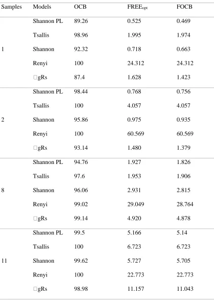
The introduced statistics with HBMES-2 were obtained for 23 of sample for all entropy models, some of which are presented in Table 2. In the first column of this table, the OCB

statistic shows the minimum CB that represents all measured data. The lower the OCB value, the higher the model’s certainty in the shear stress prediction. The FREEopt statistic, which is the

total distance of the measured data of the OCB, represents the width of OCB. If this value is lower for a model, the certainty of this model is higher.

As mentioned before, the OCB criterion can be considered as a quantitative criterion for determining the certainty of a model. Also, FREEopt is a qualitative criterion to evaluate the

uncertainty of models. The third column of Table 2 is the value that shows the combined effect of OCB and FREEopt, which is considered as the main criterion in this study as (FOCB) (FREEopt

and OCB).

Therefore, it is sufficient to find only the FOCB statistic for evaluating the uncertainty of shear stress predictor models. As can be seen in the last column of Table 2, the overall uncertainties of all models decrease with an increasing amount of water and sediment in the channel bed (h+t). In all samples, the FOCB statistic has the lowest value for the Shannon PL entropy and the highest value for the Renyi entropy, as a result, among the proposed models, Shannon PL models showed the highest certainty, and the Renyi has the lowest certainty.

(24)

the three samples 1, 2, and 11, the entropies of Shannon, ρgRs, and Tsallis have the lowest amount of the FOCB and the highest certainty, respectively. In samples 8 and 11, the values of the FOCB for the three entropies Shannon, ρgRs, and Tsallis are also close together, indicating an almost identical degree of certainty for these models.

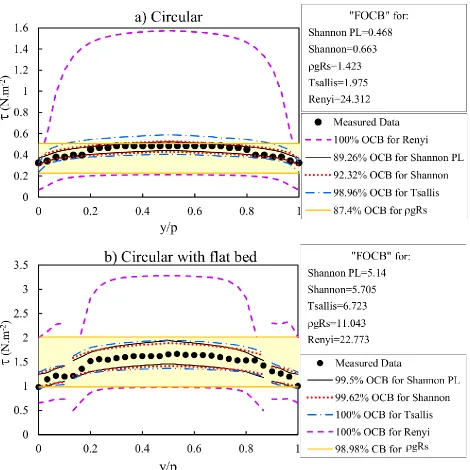
To illustrate the uncertainty statistics presented in Table 3, the OCB for two samples 1 and 11 is shown in Figure 7. Figure 7 shows the minimum confidence bound that covers all measured shear stress, OCB, for four entropy models and ρgRs model. The Figure 7a corresponds to Sample 1 for a circular channel (t/D = 0, h+t/D = 0.333) and the Figure 7b also relates to sample 11 for a circular with flatbed channel (t/D = 0.25, h+t/D = 0.333).

Each model, which has a higher OCB width, shows higher uncertainty in the prediction of shear stress. The width of OCB of the three entropy models of Tsallis, Shannon PL, and Shannon is very close and contains a very small region, while the Renyi entropy model has larger OCB

region compared with other three models.

Table 3. Statistical indexes based on HBMES-2 uncertainty method for four entropy models

for shear stress prediction.

(25)

In Table 3, sample 1 (t/D = 0), the OCB values for three Shannon PL, Shannon, and ρgRs models are close to each other and are less than the OCB values of two Tsallis and Renyi models. Despite the proximity of the OCB values for the two Tsallis and Renyi models, the width of OCB

for the Renyi model is much higher than Tsallis model; the FREEopt value of the Renyi model is

much larger than the other four models, which is shown in Table 3. In Figure 7b, although the

OCB values are very close to each other for all models, the width of OCB, in bed and wall of channel, for the Renyi entropy model is much larger than the four models. This issue is very clear in the (FOCB) statistics in Table 3 for all samples.

Figure 7. OCB for analyzing presented models in shear stress prediction by HBMES-2 uncertainty method in height ratios (a) t/D=0, h+t/D=0.333; and (b) t/D=0.25; h+t/D=0.333).

In Table 4, the values of this statistic are given for all models for the studied cases. These values show that the certainty of all models to calculating shear stress in a circular channel is much higher than in circular with flatbed channel. Except for the Renyi entropy with identical almost values for FOCB, it indicates the same uncertainty in the prediction of shear stress values. In Table 4, the values of FOCB for the Renyi entropy in both circular and circular with flatbed channels are much higher than in the other models. Given that the ρgRs model has been

(26)

The models are more certain for Shannon, Shannon PL, ρgRs, and Tsallis models to predicting shear stress in circular with flatbed channel, respectively. Finally, considering the number of samples presented in Table 1, the average values in Table 4 are given for the entire circular channel. The average values indicate that Shannon, Shannon PL, ρgRs and Tsallis models have the most certainty to estimating shear stress in the circular channels, respectively.

Table 4. The values of FOCB in circular and circular with flatbed channels for all entropy models to predicting shear stress distribution.

4. Conclusion

In this study, we present the uncertainty of four popular entropy models, including Shannon, Shannon PL, Tsallis, and Renyi have been analyzed for calculating shear stress in circular channels. The uncertainty analysis method of Kazemian-Kale-Kale et al. [46] based on the Bayesian Monte-Carlo technique was employed and named in this study as HBMES-1. However, using the HBMES-1 method along with the Nin statistic required three additional statistics (FP,

FN, and FREE) to compare the uncertainty of the model, it was not feasible to rank the

uncertainty of several models. For this reason, in the proposed new HBMES-2 method, the minimum CB that covers all measured data and the OCB were obtained, and a new statistic called FOCB was introduced to evaluate the uncertainty. The FOCB indicates the degree of uncertainty as both a qualitative and a quantitative index. Calibrations for both HBMES-1 and HBMES-2 methods were performed in different sample sizes and under different hydraulic conditions. Based on the percentage of measured data within the confidence bound (Nin), the best

(27)

standard deviation changes of the error distribution of normalized shear stress data ( and ) of all four entropy models in different SS were investigated. The lower values, the distribution of the error is approaching to the Gaussian distribution, and the validity of the obtained uncertainty results is more reliable. The values for the entropies of Shannon, Shannon PL, Tsallis, and Renyi, were 0.09, 0.06, 0.08, and 0.21, respectively. The absolute values of for the entropies of Shannon PL, Tsallis, Shannon, and Renyi, were 0.001, 0.003, 0.055, and 0.114, respectively. Applying the Box-Cox function transfer factor in the best SS selected from the model

calibration, the final evaluation was performed using two uncertainty methods. In the HBMES-1 method, it was found that all four entropy models with a percentage of measured data within 95% CB higher than 93% along with the ρgRs conventional model have high certainty in predicting shear stress in circular channels. According to the results of HBMES-2 method in a circular channel, the entropies of Shannon PL, ρgRs, Shannon, Tsallis, and Renyi with the FOCB

values were 1.339, 2.026, 2.432, 2.961, and 58.457, respectively. In the circular flatbed channel, the entropies of Shannon PL, Shannon, ρgRs, Tsallis, and Renyi, the FOCB values were 10.118, 11.591, 17.115, 17.407, and 57.565, respectively. According to the mean results of FOCB in different hydraulic conditions, it was generally found that the Shannon PL, Shannon, ρgRs, Tsallis, and Renyi models have the highest certainty in shear stress of circular channels with

(28)

References

[1] Kleijwegt, R.A. On sediment transport in circular sewers with non-cohesive deposits. Ph.D. Thesis, Delft University of Technology, Delft, Netherlands, 1992.

[2] Knight, D.W.; Sterling, M. Boundary shear in circular pipes running partially full. Journal of Hydraulic Engineering 2000, 126 (4), 263–275.

[3] Perrusquia, G. Bedload Transport in Storm Sewers. Stream Traction in Pipe Channels. Ph.D. Thesis, Chalmers University of Technology, Gothenburg, Sweden, 1991.

[4] Berlamont, J.E.; Trouw, K.; Luyckx, G. Shear stress distribution in partially filled pipes. Journal of Hydraulic Engineering 2003, 129 (9), 697–705.

[5] Bares, V.; Jirak, J.; Pollert, J. Bottom shear stress in unsteady sewer flow. Water Science & Technology 2006, 54 (6–7), 93–100.

[6] Yu, G.; Tan, S.K. Estimation of boundary shear stress distribution in open channels using flownet. Journal of Hydraulic Research 2007, 45, 486–496.

[7] Khozani, Z.S.; Bonakdari, H.; Zaji, A.H. Estimating the shear stress distribution in circular channels based on the randomized neural networks technique. Applied Soft Computing 2017, 58, 441–448.

[8] Khozani, Z.S.; Bonakdari, H.; Ebtehaj, I. An analysis of shear stress distribution in circular channels with sediment deposition based on Gene Expression

(29)

[9] Farina, G.; Alvisi, S.; Franchini, M.; Moramarco, T. Three methods for estimating the entropy parameter M based on a decreasing number of velocity measurements in a river cross-section. Entropy 2014, 16(5), 2512-2529.

[10] Kumbhakar, M.; Kundu, S.; Ghoshal, K. Hindered settling velocity in particle-fluid mixture: a theoretical study using the entropy concept. Journal of Hydraulic Engineering 2017, 143(11), 06017019.

[11] James, R.D.; Nota, A.; Velázquez, J.J. Self-similar profiles for homoenergetic solutions of the Boltzmann equation: particle velocity distribution and entropy. Archive for Rational Mechanics and Analysis 2019, 231(2), 787-843.

[12] Gholami, A.; Bonakdari, H.; Mohammadian, M.; Zaji, A.H.; Gharabaghi, B. Assessment of geomorphological bank evolution of the alluvial threshold rivers based on entropy concept parameters. Hydrological Sciences Journal 2019a, 64(7), 856-872. [13] Gholami, A.; Bonakdari, H.; Mohammadian, M. Enhanced formulation of the

probability principle based on maximum entropy to design the bank profile of channels in geomorphic threshold. Stochastic Environmental Research and Risk Assessment. 2019b, 1-22.

[14] Gholami, A.; Bonakdari, H.; Mohammadian, A. A method based on the Tsallis entropy for characterizing threshold channel bank profiles. Physica A: Statistical Mechanics and its Applications 2019c, 526, 121089.

[15] Bonakdari, H.; Tooshmalani, M.; Sheikh, Z. Predicting shear stress distribution in rectangular channels using entropy concept. International Journal of Engineering 2015,

(30)

[16] Chiu, C.L. Entropy and probability concepts in hydraulics. Journal of Hydraulic Engineering 1987, 113, 583–599.

[17] Sterling, M.; Knight, D.W. An attempt at using the entropy approach to predict the transverse distribution of boundary shear stress in open channel flow. Stochastic Environmental Research and Risk Assessment 2002, 16(2), 127–142.

[18] Sheikh, Z.; Bonakdari, H. Prediction of boundary shear stress in circular and trapezoidal channels with entropy concept. Urban Water Journal 2015, 13(6), 629–636. [19] Ghoshal, K.; Kumbhakar, M.; Singh, V.P. Distribution of sediment concentration

in debris flow using Rényi entropy. Physica A: Statistical Mechanics and its Applications 2019, 521, 267-281.

[20] Tsallis, C. Possible generalization of Boltzmann–Gibbs statistics. Journal of Statistical Physics 1988, 52(1–2), 479–487.

[21] Rényi, A. On measures of entropy and information. Proc. Fourth Berkeley Symp. on Math. Statist. and Prob., Vol. 1 (Univ. of Calif. Press, 1961), 547-561, 1961.

[22] Tsallis, C.; Brigatti, E. Nonextensive statistical mechanics: A brief introduction. Continuum Mechanics and Thermodynamics 2004, 16(3), 223-235. [23] Tsallis, C. Introduction to nonextensive statistical mechanics: approaching a

complex world. Springer-Verlag, New York, USA, 2009.

(31)

[25] Khozani, Z.S.; Bonakdari, H. Formulating the shear stress distribution in circular open channels based on the Renyi entropy. Physica A: Statistical Mechanics and its Applications 2018, 490, 114–126.

[26] Arnaud, P., Cantet, P.; Odry, J. Uncertainties of flood frequency estimation approaches based on continuous simulation using data resampling. Journal of Hydrology 2017, 554, 360-369.

[27] Baldassarre, G.D.; Montanari, A. Uncertainty in river discharge observations: a quantitative analysis. Hydrology and Earth System Sciences 2009, 13(6), 913-921. [28] Beven, K.; Lamb. R. The uncertainty cascade in model fusion. Geological

Society, London, Special Publications 2017, 408(1), 255-266.

[29] Gabellani, S.; Boni, G.; Ferraris, L.; Hardenberg, J.V.; Provenzale, A.

Propagation of uncertainty from rainfall to runoff: A case study with a stochastic rainfall generator. Advances in Water Resources 2007, 30(10), 2061-2071.

[30] Gholami, A.; Bonakdari, H.; Ebtehaj, I.; Mohammadian, M.; Gharabaghi, B.; Khodashenas, S.R. Uncertainty analysis of intelligent model of hybrid genetic algorithm and particle swarm optimization with ANFIS to predict threshold bank profile shape based on digital laser approach sensing. Measurement 2018a, 121, 294–303.

[31] Gholami, A.; Bonakdari, H.; Zaji, A.H.; Akhtari, A.A. A comparison of artificial intelligence-based classification techniques in predicting flow variables in sharp curved channels. Engineering with Computers 2019d, 1-30.

(32)

[33] Hamilton, A.S.; Moore, R.D. Quantifying uncertainty in streamflow records. Canadian Water Resources Journal 2012, 37(1), 3-21.

[34] Iskra, I.; Droste, R. Parameter uncertainty of a watershed model. Canadian Water Resources Journal 2008, 33(1), 5-22.

[35] Iyer, V.A.; Woodmansee, M.A. Uncertainty analysis of laser-doppler-velocimetry measurements fin a swirling flowfield. The American institute of Aeronautics and

Astronautics 2005, 43(3), 512-519.

[36] Misirli, F.; Gupta, H.V.; Sorooshian, S.; Thiemann, M. Bayesian recursive estimation of parameter and output uncertainty for watershed models. Calibration of Watershed Models 2003, 113–124.

[37] Montanari, A.; Brath, A. A stochastic approach for assessing the uncertainty of rainfall‐runoff simulations. Water Resources Research 2004, 40(1).

[38] Sattar, A.M.; Gharabaghi, B; McBean, E. Prediction of Timing of Watermain Failure Using Gene Expression Models. Water Resources Management 2016, 30(5), 1635-1651.

[39] Thompson, J.; Sattar, A.M.; Gharabaghi, B.; Richard, W. Event based total suspended sediment particle size distribution model. Journal of Hydrology 2016, 536, 236-246.

[40] Watt, W.E.; Paine, J.D. Flood risk mapping in Canada: 1. Uncertainty considerations. Canadian Water Resources Journal 1992, 17(2), 129-138. [41] Lamb, R.; Beven, K.; Myrabø, S. Use of spatially distributed water table

(33)

[42] Corato, G.; Melone, F.; Moramarco, T.; Singh, V.P. Uncertainty analysis of flow velocity estimation by a simplified entropy model. Hydrology Processes 2014, 28(3), 581–590.

[43] Moramarco, T.; Saltalippi, C.; Singh, V.P. Velocity profiles assessment in natural channels during high floods. Hydrology Research 2011, 42(2-3), 162-170.

[44] Rincon, R.A.C. Evaluation of uncertainty in hydrodynamic modeling. PhD. Thesis, Mississippi State University, USA, 2013.

[45] Kazemian-Kale-Kale, A.; Bonakdari, H.; Gholami, A.; Khozani, Z.S.; Akhtari, A.A.; Gharabaghi, B. Uncertainty analysis of shear stress estimation in circular channels by Tsallis entropy. Physica A: Statistical Mechanics and its Applications 2018, 510, 558-576.

[46] Kazemian-Kale-Kale, A.; Bonakdari, H.; Gholami, A.; Gharabaghi, B. The uncertainty of the Shannon entropy model for shear stress distribution in circular channels. International Journal of Sediment Research 2020, 35(1), 57-68.

[47] Knight, D.W.; Yuen, K.W.H.; Alhamid, A.A.I. Boundary shear stress

distributions in open channel flow. Physical Mechanisms of mixing and Transport in the Environment, John Wiley, New York, USA, 1993.

[48] Sterling, M. A Study of Boundary Shear Stress, Flow Resistance and the Free Overfall in Open Channels with a Circular Cross-Section. Ph.D. dissertation, University of Birmingham, Birmingham, UK, 1998.

(34)

(35)

(36)

Figure 2. Process of assessment of the OCBn(minimum confidence bound that covers all

(37)

(38)

(39)

(40)

(41)

(42)

Table 1. Summary of the main hydraulic parameters in the circular channel with and without sediment

Q(l.s-1) Fr