Inventory Management Models with Return Flows
Adwait Singhai
Department of Production and Industrial Engineering, Mechanical Department, IIT DELHI
Abstract
Inventory management has become essential to manufacturing companies as the volume of production has been surging at great pace. With the concept of “reuse” and “recycle” being adopted by most manufacturing circles to address the environmental concerns as well as reduce the cost of production, traditional inventory models have been rendered ineffective. Inventory Models with return flows are being researched and adopted. This paper reviews schematically all the inventory models dealing with return flows into the supply chain.
Keywords: Return Flows, Reverse Logistics, Recovery Process, Remanufacturable Inventory Modes25T .
1. Introduction
In recent years there has been increased attention in integrating return flows in traditional production processes. The return flows have gained significant attention because of two main reasons: Environmental concern and modern technology making recovery of used products economically more attractive. While the reuse of products and materials is not new to industries; metal scrap reuse, waste paper recycling, P.E.T bottle recycling have been around a long time; the increase in re-manufacturable inventory as a percentage of serviceable inventory in recent times has made the need for traditional models to adapt to these changes. Various academicians have grasped this stark change in inventory models cutting across all sectors of industries and developed new models with various underlying mathematical assumptions. These assumptions have been dealt with in different research papers.
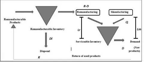
A general framework for this situation has been depicted in the Figure1: The products are manufactured in order to meet the demands, while the used products are returned to the producers after prescribed life cycle or damage or if they are rendered useless. To fill the serviceable inventory which is exhausted (partially) in meeting the demands, there are two alternatives. Either the required raw material is ordered and new products fabricated or old products overhauledand brought to ‘as new’ conditions. The objective of the inventory management is to control external demand orders and the internal inventory levels; internal component recovery process and/or new material
procurement and storage process; to guarantee a required service level and to minimise the fixed and variable costs.
Figure 1: A hybrid system with manufacturing and remanufacturing operations and stocking points for remanufacturables and serviceable
The return of the used products has different types: repair, refurbishing, remanufacturing and recycling. [1]. Repair returns a used item to working order. Refurbishing brings an item up to a specified quality. Remanufacturing brings an item to ‘as new’ quality. Recycling is using the waste product as a raw material for another process. In case of direct reuse the recovery process may vanish completely, with returned products directly entering serviceable inventory. In case of recycling, if there is no alternative raw material source, traditional models apply well. This paper focuses on recovery processes, therefore repair, refurbishing and remanufacturing. Recovery process as already stated is an alternative to manufacturing processes.
The producer typically has little control on the return flow in terms of quantity, quality and timing. The effects of return flow in this situation are twofold. On one hand it may be cheaper to overhaul an old product than to produce a new one. On the other hand reliable planning becomes more difficult due to increased uncertainty which may lead to higher safety stock levels. To avoid excess inventory of used products disposal may be an additional option.
demands have to be satisfied by manufactured (new) products.
Let us elucidate on the random variables involved in the model as shown in figure 2:
Figure 2: Random variables in Inventory model for hybrid systems
R: Real time stochastic variable i.e the time varying return of items
Di: Real time varying process of Disposal
Lr: Lead time for remanufacturing, stochastic variable Lm: Lead time for manufacturing, stochastic model Q: Real time varying process of Manufacturing D: Demand variable
Several authors have considered different types of models, treating the Random Variables differently. The easiest types of model have zero lead times and continuous and deterministic demand and return rates without any disposal. Some complex models consider the demand and return rates to be stochastic processes without considering the disposal. The effect of lead times under simple PUSH and PULL control strategies has also been considered extensively.[2]. In the sequel we discuss the proposed models which mainly differ with respect to assumptions on demand and return processes and on recovery process.
2.
Inventory Models
A first major classification can be made into deterministic versus stochastic inventory models.
2.1 Deterministic Models
In deterministic inventory models information on all the components of the framework presentedin Figure 2 is assumed to be known with certainty. In particular, demands and returns are knownin advance for every point in time. The objective is to strike an optimal trade–off between fixedsetup costs and variable inventory holding costs. This corresponds to the mind-set of the basicEOQ formula in classical inventory theory. Several authors have
proposed modifications to thisformula taking return flows into account.
The main advantage of EOQ (Economic Order Quantity) model is that, due to their simplicity, they lead to closed-form expressions for the optimal batch sizes. Of course, the strong underlying assumptions are not realistic. But, as is usual in traditional inventory systems with manufacturing only, the EOQs can be used as approximation in more realistic models.
Schardy[3]was the first who analysed an EOQ model with recovery. The model is based on the assumption that the manufacturing and recovery rate are infinite. Policies with fixed batch sizes 𝑄𝑚 for manufacturing and 𝑄𝑟 for recovery are considered, where one manufacturing batch is always succeeded by R recovery batches. Disposal is not allowed, i.e. all returned items are recovered. Simple square root formulas for 𝑄𝑚and 𝑄𝑟 are derived working on the model with before mentioned assumptions.
Mabini, Pinteln, and Gelders[4] discuss the formulations of the EOQ type for controlling inventories of repairable items. They subsequently consider two problem situations. Assuming infinite repair capacity and a fixed disposal rate (scrapping rate), they deal with the single item case. The model is subsequently modified to account for multiple items that share a common and limited repair capacity. This is the major development over Schardy’s [2] model.
Richter [5][6]considers and EOQ model with the stationary demand being satisfied by the manufactured products and the recovered items. The model is based on the assumption that the returned products are collected in a “second shop” and repaired later, after a collection period, at some fixed rate. Disposal of other products is also included according to some constant waste disposal rate. This model essentially extends previous studies to the case of variable setup numbers ‘N’ and ‘M’ for production and repair within variable collection time interval. This collection interval coincides with a production cycle and leads to extra holding costs, since recovery is postponed. Richter determines the cost optimal setup numbers and minimum cost for a fixed disposal rate.
Teunter[7] generalizes Schardy’s result. A policy with ‘M’ manufacturing batches and ‘R’ recovery batches is considered. The model also includes a variable disposal rate. The holding costs for manufactures and recovered items are distinguished in the model. One of the major assumption of his model, to derive an expression, is to set either M=1 or R=1. He then determines the optimal policy for fixed batch sizes 𝑄𝑚 for manufacturing and 𝑄𝑟 for recovery and ‘λu’ rate of reuse.
2.2 Stochastic Models
In this section inventory models that treat demand, return, disposal and rate of return as stochastic processes are discussed. The Product Recover systems have been studied in this paper, omitting the Repair systems. Repair systems have demand and returnprocesses perfectly correlated and therefore there is no increase in totally inventory on hand.
2.2.1 Product Recovery Systems
In hybrid systems coordination between the remanufacturing and manufacturing activities and thus the two inventory levels are central to policy making. The demand and return are independent stochastic processes due to large population and large variability in population. To present a proper structure of review we have distinguished the models into periodic review models, the status of system is reviewed after discrete intervals, and continuous review models, in which as the name suggests the system is reviewed continuously. The two control strategies, namely the PUSH and PULL control strategies will be further discussed.
Periodic review model
The earliest work was done by Simpson [8]. His proposed model assumes mutually dependant demand and return stochastic processes. The research paper considers the reuse of returned items and the associated material savings versus the inventory holding costs of manufactural raw material. This model however has following limitations: the lead times for remanufacturing and procurement of fabricated material from outside are assumed to be zero. Also, the costs of procuring fabricated material from outside and fixed manufacturing are taken to be zero.
Inderfurth[9] has continued the work of Simpson by incorporating non-zero lead times for order and recovery processes. He compares the lead times for the two processes and concludes that the difference between the two lead times determines the complexity of the system. His model is a general case of Simpson’s where identical lead times result into a model to similar while for different
lead times the growing dimensionality of the underlying Markov model prohibits simple optimal control rules.
Kelle and Silver [10] formulated a different model with independent demand and return processes, zero disposal rates i.e. all returned items being remanufactured and PUSH-strategy in remanufacturing. Based on net demand per period they formulate a chance constrained integer program. They approximate the problem into classical dynamic lot sizing problem. Their model includes service level constraints and fixed ordering costs.
We have discussed single item inventory systems until now. Multi item hybrid systems have also been studied. Brayman[11] and Flapper[12] have put forth MRP policies discussing the complexities in multi item hybrid systems.
Continuous Review Models
Heyman[13] was among the firsts to propose continuous review model. The model assumes the demand and return processes to be stochastic variables and uncorrelated. Returned items are either recovered or remanufactured with zero lead time or disposed of with zero disposal lead times. He essentially analyses the trade-off between savings of production costs and additional costs of holding inventory. He considers recovery process and outside procurement to be instantaneous and therefore a perfect service system with single inventory. He omits the fixed cost. The system is controlled by a single-parameter (𝑠𝑑) PUSH strategy. Parameter ′𝑠𝑑′ is the level of serviceable inventory exceeding which incoming remanufacturablesare disposed of.Heyman argues the equivalence of this model to M/M/1/∞ or a single server queueing model. Assuming the return and demand processes to be Poisson distributed, he derives an expression for optimal disposal level (𝑠𝑑) . He approximates a model for generally distributed demands and returns and proves the optimality of one parameter policy.
serviceable inventory level 𝑠𝑝 at which an order of manufacturing lot size 𝑄𝑝 is placed.
Van der Lan et al.[15][16][17]present an alternate approximation for Muckstadt and Issacs’s single echelon model based on the net demand during the manufacturing lead times and a numerical comparison showing the accuracy of this approach. The number of remanufacturables in the inventory is kept to a maximum level of N thus providing for disposal. Van der Laan et al also presents a numerical comparison of various disposal strategies and show disposal decisions based on both serviceable and remanufacturable inventory levels is more advantageous. PUSH and PULL strategies are also defined and effects of lead time variability of remanufacturing and manufacturing on expected costs are numerically compared.
Kismuller[18]discusses the PULL control policy to integrate the manufacturing and remanufacturing inventory with optimal results. The system is classified based on lead times. In larger remanufacturing lead time systems, manufacturing quantity is determined first followed by quantity of recycled products to be ordered by considering net serviceable and all outstanding production and remanufacturing order. Whereas, larger manufacturing lead time systems need to consider recoverable on hand inventory also.
[19] A more detailed model for hybrid system inventory has been described by Van der Laan, Fleischmann, & Dekker.
The model is based on conditions such as correlation between return and demand processes and stochastic lead times. The description of the model can be explained taking into consideration the stochastic demand and return flows, which is modelled by Markovian arrival process. In case of product disposal, there are two scenarios, first, if disposal of product is not allowed than an assumption of return intensity (the average number of returns per unit of time) is less than demand intensity and vice versa. Also, the framework enables to investigate the influence of other system parameter, such as the holding cost structure. It was also figured out that characterization of manufacturing and remanufacturing lead time plays a significant role in controlling policy.
Inderfurth[20] proposes the hybrid inventory model to be slightly different from previous versions. The returned product is accumulated in used product inventory (UP Inv.) until remanufacturing process start. Returned product that meets all the standards are allowed to move to remanufacturing process, while others are collected in
disposal. The result of remanufacturing process is collected in Remanufacturing Inventory (RP Inv). If the RP cannot fulfil all the market demand, company manufactures new product and it is collected in Manufacturing Inventory (MP inv)which is then combined with RP inventory to satisfy market demand.
Other researcher, Aras, Verter and Boyaci[21]modelledthe hybrid system with uncertain quality of returns.They integrate the manufacturing facility, including a new component /raw material inventory stocking point. They model manufacturing with constant unit processing costs, and constant procurement and manufacturing lead times, in order to highlight the impact of remanufacturing uncertainties. A simulation-based optimization framework is used to show the basic setting, the two prioritization strategies priority-to-manufacturing (PTM) strategy and priority-to-remanufacturing (PTR) strategy are compared. If priority is given to manufacturing, a replenishment order is placed first with the manufacturing facility and remanufacturing is used only when manufacturing is not possible due to insufficient inventory of new components. They refer to this strategy as priority-to-manufacturing (PTM) strategy in the sequel. The alternative strategy is the priority-to-remanufacturing (PTR) strategy, which (as in existing models) places a replenishment order to remanufacturing and resorts to manufacturing only if the remanufacturable inventory is empty.
3.
Conclusions
Determination of optimal control policy in a hybrid system with integrated remanufacturing and manufacturing processes has been the main objective of the above models. Different assumptions have been applied in different models according to the case scenario. The different models have scope to develop different combinations of PUSH and PULL system and continuous or periodic review. A model with continuous review system and PUSH control policy in remanufacturing and periodic review system and PULL control policy in manufacturing still needs to defined in detail. Various proposed models need to be analysed and evaluated using simulations based on optimisation. Using simulations, control policies of hybrid inventory systems can be analysed for continuous improvement.
References
[1] R.H. Teunter, “Economic Ordering Quantities for Recoverable Item Inventory Systems,” 2001.
[3] D. A. Schardy, “A deterministic inventory model for repairable items,” Nav Res Logistics Quart 14, 1967, pp. 391-398,
[4] M.C. Mabini, L. M. Pintelon and L. F. Gelders, “EOQ type formulations for controlling repairable inventories,” International Journal of Production Economics, 1998. [5] K. Richter, “The extended EOQ repair and waste disposal
model,” International Journal of Production Economics, 1996, pp. 443-448.
[6] K. Richter, “The EOQ and waste disposal model with variable setup numbers,” European Journal of Operational Research, 1996, pp. 313-324.
[7] R. H. Teunter, “Economic Ordering Quantities for Recoverable Item Inventory Systems,” Naval Research Logistics, 2001, pp. 484-495.
[8] V. P. Simpson, “Optimum solution structure for repairable inventory problem,” Operations Research, 1978, pp. 270-281.
[9] K. Inderfurth, “Simple optimal Replenishment and disposal policies for a product recovery system with leadtimes,” OR Spektrum, 1997, pp. 111-122.
[10] P. Kelle and E. A. Silver, “Purchasing policy of new containers considering the,” IIE Transactions, 1989, pp. 349-354.
[11] R. D. Brayman, “How to implement MRP IIsuccessfully the second time: getting people involved int the remanufacturing environment,” in APICS Remnaufacturing Seminar Proceedings, 1992.
[12] S. D. Flapper, “Matching material requirements and availabilities in the context of recycling: an MRP-I based heuristics,” in Proceedings of the Eight International Working Seminar on Production Economics, Iglis/Innsburck, 1994.
[13] D. P. Heyman, “Optimal disposal policies for a single-item inventory system with returns,” Naval Research Logistics Quarterly, 1977, pp. 385-405.
[14] J. Muckstadt and M. H. Issac, “An analysis of single item inventory systems with returns,” Naval Research Logistics Quarterly, 1981 pp. 237-254.
[15] E. Van der Laan, On inventory control models where items are remanufactured or disposed, Master's thesis, Erasmus University Rotterdam, The Netherlands, 1993.
[16] E. Van der Laan, R. Dekker and M. Salomon, “n (s,Q) inventory model with remanufacturing and disposal,” International Journal of Production Economics,, 1996a. [17] E. Van der Laan, R. Dekker and M. Salomon, “Product
remanufacturing and disposal: A numerical comparison of alternative control strategies,” International Journal of Production Economics, 1996b, pp. 489-498.
[18] G. P. Kiesmuller, “Kiesmuller, A new approach for controlling a hybrid stochastic manufacturing/remanufacturing system with inventories and
different lead times,” European Journal of Operational Research, 2003, pp. 62-71.
[19] E. Van der Laan, M. Fleischmann and R. Dekker, “Inventory control for joint manufacturing and remanufacturing, in Quantitative models for supply chain management,” Kluwer Academic Publisher, Massachusetts, 2003.
[20] K. Inderfurth, “Optimal policies in hybrid manufacturing/remanufacturing systems with product
substitution,” International Journal Production Economics,2004, pp. 325-343.
[21]N. Aras, V. Verter and T. Boyaci, “‘Coordination and priority decisions in hybrid manufacturing/remanufacturing systems,” Production and Operations Management, 2006, pp. 528-543.
First AuthorAdwait Singhai is a senior undergraduate in Production and Industrial engineering in Indian Institute of Technology, Delhi. He has been a recipient of prestigious scholarships, National Talent Search Examination and the Kishore VyagnikProsthahanYojna conducted by