www.ijiset.com
120
Modeling and experiment of the Wave
Generated by an Oscillating Wedge-shaped
Ha PhuongP*
P
, Quoc Thanh TruongP
*
PR, RDoan Son TranP
*
P
*
P
Ho Chi Minh University of Technology, Vietnam National University HCM 268 Ly Thuong Kiet, District 10, Ho Chi Minh City, Vietnam
ABSTRACT: This paper describes modeling and fabrication of a wave flume and that associate with the equipment. Wave flume is equipped with a triangle wedge that locates at the one of the end a channel and the passive wave absorber is located at the other end for absorbing waves generating from the wave maker. The wedge is controlled by a desktop computer, it can move up and down at a prescribed speed and oscillation amplitude corresponding to the desired wave height and frequency. At the middle flume is equipped micro laser distance sensor which provides data-logging capability. Wave flume can generate the largest waves are about 0.2 meter high, have a period about 1 second, and have a wavelength about 1.5 meters. The waves generated by a oscillating wedge and modeling have been measured, analyzed to consider the generated wave energy.
Index Term - Wave Energy, Wave Flume, Wave Generation, Wave Maker
1. INTRODUCTION
Ocean wave energy is the natural resource to be exploited as a renewable source of energy, while also coinciding with the aim of reducing our reliance on fossil fuel sources. The concept of harnessing ocean wave energy is by no means a new idea. Modern research into harnessing energy from waves was stimulated by the emerging oil crisis of the 1970s [1]. With global attention now being drawn to climate change and the rising level of COR2R, the focus on generating electricity from renewable sources is once again an important area of research. At present, many countries in the world use wave energy as a source of clean and renewable energy [2] [3] (fig.1)
Fig.1. Some of typical wave energy converter on over the world
121
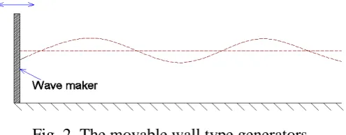
motion with specified amplitude and frequency [4]. Three main classes of mechanical type wavemakers are utilized in laboratory: The first is the movable wall type generators [5], including piston and paddle-type wavemaker, which generates waves by a simple oscillatory motion in the direction of wave propagation (fig 2). The movable wall type generators are used where the water is shallow compared to the wavelength of the waves. Here the orbital particle motion is compressed into an ellipse and there is significant horizontal motion on floor of the tank. This type of paddle is used to generate waves for modelling coastal structures, harbours and shore mounted wave energy devices.
Fig. 2. The movable wall type generators
The second is the plunger-type wavemakers [5], which generates waves by oscillating vertically in the surface of water (fig 3). The plunger-type wavemakers are commonly used in wave flumes because they can be fabricated as fairly long wave machines and they easily relocated within the the flumes. The machine is very compact, furthermore, as the shape is wedge, the flume can be designed to work with water behind the wave maker with almost no generation of back waves [4]
Fig. 3. The plunger-type wavemakers
The third is the flap-type wave-maker, which is located at one end of the tank [6], and hinged on a sill (fig 4), waves are generated by oscillation of the flap about the sill, flap-type wave-maker is used to produce deep water waves where the orbital particle motion decays with depth and there is negligible motion at the bottom.
Fig. 4. Flap-type wave-maker
www.ijiset.com
122 2. NUMBERICAL METHOD
19T
2.1 Numerical model description
The main software used in this work is Ansys which has an extensive range of features to solve technical issues, i.g solid dynamics, electromagnetic problems, fluid mechanics,.. The governing equations used in this software are the continuity equation, energy equation, energy conservation equation and momentum equation. The Navier-Stokes equation is the combination of those equation. The Navier-Stokes equation used for incompressible and a Newtonian fluid:
(1)
In which ρ is the density of the fluid (kg/mP
3
P
, u is the velocity of the fluid (m/s), p is the pressure (N/mP
2
P
), g is the acceleration of gravity (m/sP
2
P
), µ is the dynamic viscosity, t is the time (s), ∇P
2
P
is Laplacian vector.
In this modeling used the k-ε model which quite popular. This is a model of two equations to describe turbulent flows. The first equation is the turbulent kinetic equation k to determine the turbulent energy, the second equation is the turbulence dissipation equation ε to determine the turbulence scale [7]. This model is suitable for small pressure gradient, so it is suitable for waveforming channel with little pressure change (about 3.9 Kpa). The k-ε model [8]:
𝜕𝑡𝜕 (𝜌𝑘) +𝜕𝑥𝜕
𝑖(𝜌𝑘𝑢𝑖) =
𝜕 𝜕𝑥𝑗��
𝜇𝑡
𝜎𝑘�
𝜕𝑘
𝜕𝑥𝑗�+ 2𝜇𝑡𝐸𝑖𝑗𝐸𝑖𝑗− 𝜌ε (2)
𝜕𝑡𝜕 (𝜌𝜀) +𝜕𝑥𝜕
𝑖(𝜌𝜀𝑢𝑖) =
𝜕 𝜕𝑥𝑗��
𝜇𝑡
𝜎𝜀�
𝜕𝜀
𝜕𝑥𝑗�+𝐶1𝜀
𝜀
𝑘2𝜇𝑡𝐸𝑖𝑗𝐸𝑖𝑗 − 𝐶2𝜀𝜌 𝜀2
𝑘 (3)
In which K is turbulent kinetic, ε turbulence dissipation, the deformation ratio and is eddy viscosity:
(4)
These are the correction factors.
19T
The Volume Of Fluid (VOF) method is used to19T 19Ttrack the free surface elevation. This method determines the fraction of each fluid that exists in each19T19Tcell. The equation for the volume fraction is:
∂α
∂t +∇. (αU) = 0 (5)
19T
where 19T21TU 19T21Tis the velocity field, 19T22Ta19T22Tis the volume fraction of water in the cell and varies from 0 to 1, full19T19Tof air to full of water, respectively
19T
2.2. Numerical model setup
19T
123
Fig. 5. Cheme of the wave tank.
19T
Step 2: We divided the model into many small elements, because of the limited conditions of the computer, so the mesh is divided into a square grid and the size of each grid cell is 2cm, after the division is complete, we get 50250 mesh elements.
19T
Step 3: Set the initial condition, the simulation of the two phase case, phase 1 is the air phase, we assigned the physical properties of air to this phase, the air phase at temperature 25P
o
P
C, with a density of 1,185kg / mP
3
P
Phase 2 is the water phase (water liquid) at a temperature of 25P
o
P
C, with a density of 997 kg / mP
3
P
. We assigned the physical properties to this phase.
19T
Step 4: Set boundary conditions for simulation: with wedges defined as a wall boundary set to vertical movement in 1s cycles and 0.1m amplitude and velocity is 0.2m / s in the expression language CEL (Expression Language) in CFX. (Figure 6). The two sides of the channel are two symmetrical boundaries to minimize the friction between the tank and water. The others boundary conditions are fixed walls. Above the open surface exposed to the air, the height of the water level is 0.9 meters from the bottom to the openning of the tank.
19T
Step 5: Set the motion equation for the simulation:
19T
During the simulation process we used the CEL expression language to determine the ratio of water to air. Below the average water level is set to 1, which means that the elements are filled with water, and vice versa above the average water level is set to 0. Which means that the elements are full of air. Thus the free surface will be determined with every time step.
19T
Syntax for determining water and air volume ratio:
19T
+ For water: water if (y <900 [mm], 1,0) where y is the water depth (mm)
19T
+ For air: air 1-water
19T
+ The wave generator is set for the linear motion in a vertical direction with the equation of motion being:
yRdisR= Asin(n.t) (6)
19T
Where yRdis Ris the amount of change in the y direction, A is the wedge-shaped amplitude, n is the angular velocity n = 2.π.t; in which t is the simulation time step. The initial parameters: set the velocity in 3 directions X, Y, Z are all zero, the surface is open to air.
www.ijiset.com
124
19T
- Step 5: Proceed to the computer running simulation, this process may take several hours to several months depending on the size of the original problem and the strength of the computer (the computer running the simulation is I7, 16 Gb of ram)
19T
- Step 6: Analyze and process the results after calculation, here we will draw the necessary results for our studies (velocity, pressure, water level in each location, ...)
19T
2.3. Simulation results
19T
The wedge oscillation amplitude is set to 0.1 m with a wedge oscillation frequency is 1 Hertz. We obtained the simulation results with a wave height of 0.144m, a wave period of 0.97s and a wavelength of 1.83m as shown in Figure 7 and table 1 below.
Fig. 7. Simulation results
19T
From Figure 7, we can access the simulation results as shown in Table 1 below.
19T
Table 1. Simulation results data
3. DESIGN AND FABRICATION
19T
3.1. Wave Flume
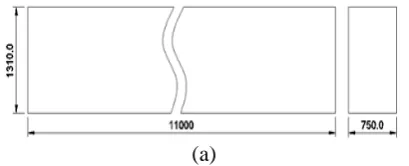
Experiments were performed in a concrete wave flume which is 0.75-meter-wide, 1.3-meter-tall and 11 meters long (Fig. 8a). The water depth was maintained at 0.97 meters. The one side of the flume is made of 1-cm-thick clear mica sheets for observe the water waveform, mica sheets are supported by steel structural frames, the other side is the concrete wall (Fig. 8b).
(a) (b)
Fig. 8. (a) Scheme of the wave flume (b) Panoramic view of the wave flume
Coordinates of points (Metric units)
Point 1 Point 2 Point 3 Point 4
X Y Z X Y Z X Y Z X Y Z
125
19T
3.2. Wave Gauges and Data Acquisition
A Micro Laser Distance Sensor (HG-C1400-Panasonic) is used for measuring the wave height. This sensor is located at the middle of the tank and it isn't contacted with water so not affect parameters of the wave. This is also the advantage of this design Additionally an Eccentricity Sensor is used to measure the wedge position (Fig. 10a).
19T
3.3. Wave-Maker
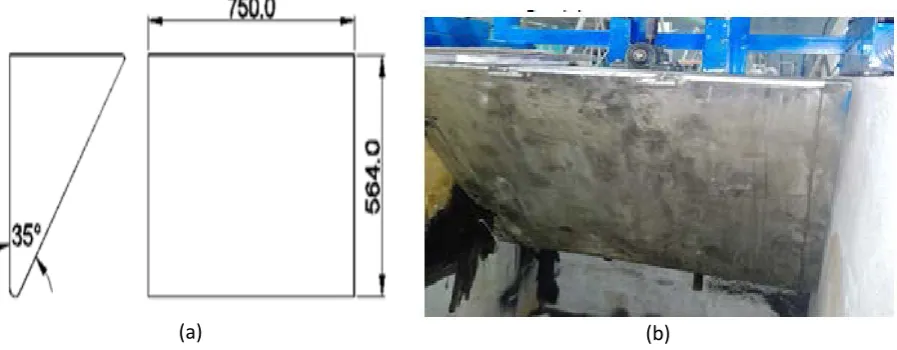
Waves were generated using a wedge shaped plunger device, the 35 degree wedge has been chosen for the wave-maker because 35 degree wedge is so good for wave-maker performace [9]. It is set at one end of the tank (Fig 10b) and is made of 1-mm-thick Inox sheets, it can generate regular waves. The wedge has a 0.418 m base and 0.566 m height, with a mean submergence height of 0.375 m (Fig 9a). The wedge is operated by 1 kW electric linear servo motor, which is controlled by computer. The installed wave-maker is capable of generating regular waves from 0.7s up to 3s period and 0.7m up to 14m wave length (case by case) . The servo motor is programmed to provide sinusoidal input motion to the Wave-Maker [10].
(a) (b)
Fig. 9. (a) Scheme of the Wave-Marker (b) Panoramic view of the Wave-Marker
www.ijiset.com
126
19T
3.4. Wave Absorber
Wave absorber is the most important part in a wave flume. A great variety of designs and materials have been used throughout the world for the construction of wave absorbers. Wave absorbers could be classified into two main categories: active and passive absorbers. Active absorbers owning to its high cost is still very limited, except in a few cases where the wave board itself is programmed to absorb the reflected wave. In this design uses passive absorbers, the wave absorber has 1:4 slopes [11]. It is located at the end of the tank opposite to the wave-maker (Fig 6c). The waves generated are absorbed using a honey comb which is set at the other one end of the tank (Fig 8).
(a)
(b)
Fig. 11. (a) Scheme of the Wave-Absorber (b) Panoramic view of the Wave-Absorber
4. THEORETICAL APPROACH
Many models can be used to try to describe the evolution of the surface elevation in time and space. One of the most used, because of the simplicity that results of assuming linearity of the potential flow function, is the one related to the linear wave theory [12].
𝜂(𝑥;𝑡) =𝐴cos (𝜔𝑡 − 𝑘𝑥) (1)
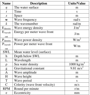
The main parameters that define a wave are amplitude (A), period (T) and wavelength (L), represented in Fig 9. The amplitude corresponds to half of the wave height (H), the vertical distance between the highest and the lowest surface elevation in a wave. The time interval between the start and the end of the wave is what is known as the period of a wave. Finally, the wavelength is the distance between two successive peaks or two consecutive troughs. Table 1 and Fig 9 summarize a commonly used wave energy nomenclature.
(b) (c)
127
Fig. 9. Sine wave pattern and associated parameters in waves.
Table 1. Wave Nomenclature
Name Description Units/Value
η The water surface m
t Time s
x Space m
w Wave frequency rad/s
k The wavenumber rad/m
ERdensity Wave energy density J/mP
2
ERwavefr
ont
Energy per meter wave front
J/m
PRdensity Wave power density W/mP
2
PRwavefr
ont
Power per meter wave front
W/m
SWL Mean water level (surface)
h Depth below SWL m
L Wavelength m
ρ Sea water density 1000 kg/mP
3
g Gravitational constant 9.81 m/sP
2
A Wave amplitude m
H Wave height m
T Wave period s
C Celerity (wave front velocity) m/s
RPM Round per minute r/m
e Eccentricity mm
Energy and power density: The energy density of a wave is the mean energy flux crossing a vertical plane parallel to a wave’s crest. The energy per wave period is the wave’s power density and can be found by dividing the energy density by the wave period.
Edensity =ρgH 2
8 =
ρgA2
2 (7)
Pdensity =Edensity𝑇 =ρgH 2
8𝑇 =
ρgA2
2𝑇 (8)
Power per meter of wave front: A wave resource is typically described in terms of power per meter of wave front (wave crest). This can be calculated by multiplying the energy density by the wave front velocity.
Pwavefront = C. Edensity=LρgH 2
8T (9)
www.ijiset.com
128 5. RESEACH METHOD, RESULT AND DISCUSSION
The research method is used in this paper is experiment method. We experiment with many diferrence parameters of system to consider the gernerated wave energy.
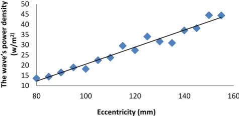
The list of experimental tests are presented in Table 2. These tests were chosen to show the wave height range of 12 mm to 200mm, wavelength range of 0.7m to 14m. The water depth was maintained at 0.97 meters.
Table 2. List of experimental tests (RPM=50 r/m)
From Table 2, we draw Fig13. According to Fig 13, we find that the wave's power density is related to eccentricity, which can be predicted linearly. May be, the experimental system is not good, So, there are many places that do not follow the linear relationship.
Fig. 12. Eccentricity efficiency
Table 3, we draw Fig 14. According to Fig 14, we see that the wave's power density is related to the RPM, which can predict as a second order. When RPM is greater than 68r/m; the waves are interrupted.
Table 3. List of experimental tests (e=80mm)
10 15 20 25 30 35 40 45 50
80 100 120 140 160
Th e w av e’ s p ow er d en si ty (w/ m 2) Eccentricity (mm) 0 5 10 15 20 25 30 35 40 45 20 30 Th e wa ve ’s p owe r d en si ty (w/ m 2)
e (mm) T (s) H (mm) L(m) PRdensity R(w/mP 2
P
)
80 0.895 99.656 1.250 13.606
85 0.895 102.661 1.251 14.434
… … … … …
145 0.896 167.101 1.254 38.197
150 0.896 180.486 1.254 44.562
155 0.894 180.023 1.249 44.430
RP M
T (s) H (mm) L (m) PRdensity R(w/mP 2
P
)
20 2.221 35.669 7.704 0.702
22 2.069 88.884 6.686 4.681
… … … … …
64 0.697 137.94 0.758 33.473
66 0.681 141.10 0.725 35.827
129
Fig. 13. RPM efficiency and Eccentricity efficiency
Table 4. List of experimental tests (e=100mm)
Fig. 14. RPM efficiency and Eccentricity efficiency
Table 4, we draw Fig 15, according to Fig 15, when increasing eccentricity (e = 100mm); the wave's power density increases. When RPM is greater than 66 r/m; the waves are interrupted.
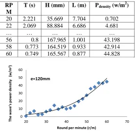
Table 5. List of experimental tests (e=120mm)
RP M
T (s) H (mm) L (m) PRdensity R(w/mP 2
P
)
20 2.221 35.669 7.704 0.702
22 2.069 88.884 6.686 4.681
… … … … …
56 0.8 167.965 1.001 43.198
58 0.773 164.519 0.933 42.914
60 0.749 165.567 0.877 44.828
Fig. 15. RPM efficiency and Eccentricity efficiency
Table 5, we draw Fig 16. In Fig 16, when e= 120, the graph has more fluctuation, due to the influence of reflectivity. When RPM is greater than 60r/m; the waves are interrupted
0 10 20 30 40 50 60 2 Th e wa ve ’s p owe r d en si ty (w/ m 2) 0 10 20 30 40 50 60
20 30 40 50 60 70
Th e wa ve ’s p owe r d en si ty (w/ m 2)
Round per minute (r/m)
e=120mm
RPM T (s) H (mm) L (m) PRdensity R(w/mP 2
P
)
20 2.217 28.202 7.673 0.439
22 2.069 74.062 6.684 3.250
… … … … …
62 0.723 161.510 0.816 44.224
64 0.698 165.402 0.761 48.034
www.ijiset.com
130
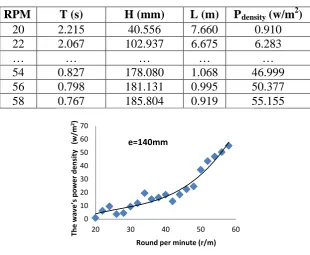
Table 6. List of experimental tests (e=140mm)
RPM T (s) H (mm) L (m) PRdensity R(w/mP
2
P
)
20 2.215 40.556 7.660 0.910
22 2.067 102.937 6.675 6.283
… … … … …
54 0.827 178.080 1.068 46.999
56 0.798 181.131 0.995 50.377
58 0.767 185.804 0.919 55.155
Fig. 16. RPM efficiency and Eccentricity efficiency
Table 6, we draw Fig 17. In Fig 17, when increasing eccentricity longer; fluctuation as much, due to the influence of reflectivity so much. When RPM is greater than 58r/m; the waves are interrupted.
Fig. 17. The influence of RPM and Eccentricity
Fig 18 Illustrate how RPM and eccentricity affect the wave’s power density. The wave’s power density is significantly affected by RPM and Eccentricity.
0 10 20 30 40 50 60 70
20 30 40 50 60
Th
e wa
ve
’s
p
owe
r d
en
si
ty
(w/
m
2)
Round per minute (r/m)
131 6. COMPARE AND EVALUATE SIMULATION RESULTS WITH EXPERIMENTAL RESULTS
19T
6.1. Experimental results
The wedge oscillation amplitude is set to 0.1 m with a wedge oscillation frequency of 1 Hertz. Based on the obtained data, we can calculate the experimental results of the wave height of 0.149m, 0.75s wave period and 1.7m wavelength.
Fig. 18 Wave height is collected
19T
6.2. Evaluation between simulation and experiment
To evaluate the results of the simulation compared to the real experimental model, we used two values: Nash – Sutcliffe model efficiency coefficient (NSE) and Xtb average error. Nash coefficient is the coefficient that shows the correlation between real measured value and simulated calculation value. The simulation gave good results when Nash was in the range of 0: 1 and the average error was less than 10%. The calculation formula:
𝑁𝑆𝐸= 1−∑𝑛𝑖=1(𝑋𝑜𝑏𝑠,𝑖−𝑋𝑠𝑖𝑚,𝑖)2
∑𝑛𝑖=1(𝑋𝑜𝑏𝑠,𝑖−𝑋�������𝑜𝑏𝑠)2 (11) 𝑋𝑡𝑏=1𝑛∑𝑛𝑖=1�𝑋𝑜𝑏𝑠𝑋,𝑖𝑜𝑏𝑠−𝑋,𝑖𝑠𝑖𝑚,𝑖�∗100 (12)
In which 𝑋𝑜𝑏𝑠,𝑖 is the measurement value on the real model, 𝑋������ is the measurement value on 𝑜𝑏𝑠 the real average model, 𝑋𝑠𝑖𝑚,𝑖, is the simulation value, n is the number of calculated values.
19T
6.2.1. Assess the wave height
To evaluate the results of the simulation compared to the real experimental model, we measure the wave height of any two points on the real model, and the wave height of any two points on the simulation (the position of the simulation and the real model is the same) we get the following evaluation table:
Table 4. Table of wave height evaluation
POINT 𝑋𝑜𝑏𝑠,𝑖(m) 𝑋������𝑜𝑏𝑠(m) 𝑋𝑠𝑖𝑚,𝑖(m) NASH
1 0.143 0.146 0.14
0.44
2 0.149 0.148
-80 -60 -40 -20 0 20 40 60 80
60 60.5 61 61.5 62 62.5 63 63.5 64 64.5 65
W
av
e h
ei
g
h
t
(mm
)
www.ijiset.com
132
The Nash value of 0.44 proves that the simulation value is quite compatible with the experimental value.
19T
6.2.2. Evaluation of wavelength
Because the wavelength is stable, we use the formula for calculating the average error. The average error calculated is 7.64, showing that the experiment and simulation are quite well correlated.
Table 5. Wavelength evaluation table
Measurement wavelength (m) Calculated wavelength (m) Average error %
1.7 1.83 7.64
19T
6.2.3. Assess the wave cycle
Because the wave period stabilizes a value, we use the formula for calculating the average error. The average error calculated is 29.33, which shows that the experiment and simulation are not correlated well.
Table 6. Table of wave cycle evaluation
Measurement cycle (s) Calculation period (s) Average error%
0.75 0.97 29.33
7. CONCLUSION
In this paper, the system wave flume is described and fabrication for a study and built with a limited budget, however, it is well-suited to educational and research studies about wave energy. The performance of the physical wave maker and wave absorber was evaluated over a range of frequencies and eccentricity. The results also show that the wave’s power density significantly affected by RPM and Eccentricity. The affected of reflectivity is so much, further work, we will improve the performance of the wave absorber in the wave flume to minimize the reflected waves.
Comparing experimental and simulation results, we find that the wave height between the two simulation and experimental cases is quite similar (Nash number 0.44), the average error for the wavelength also gives good results (7.64% ), but the error for the wave period is quite large (29.33%) due to the following reasons:
Experiment:
- Because the experimental model was not optimized.
- The channel is not long enough to stabilize the fluid flow, making the fluid flow tend to reflect back, affecting the wave cycle.
- The effect of water leakage along the canal wall.
- The absorption of wave energy is not good.
- Effect of channel roughness.
Modeling:
- The machine is not strong enough to make meshing more smooth.
133
The above defects will be overcome by us in the near future.
ACKNOWLEDGEMENTS
This research is funded by Ho Chi Minh City University of Technology-VNU-HCM under grant number T-KTXD-2019-40
REFERENCES
[1] S. H. Salter, "Wave power," Nature, vol. 249, pp. 720-724, 1974.
[2] F. d. O. Antonio, "Wave energy utilization: A review of the technologies," Renewable and sustainable energy reviews, vol. 14, pp. 899-918, 2010.
[3] E. Enferad and D. Nazarpour, Ocean's Renewable Power and Review of Technologies: Case Study Waves: INTECH Open Access Publisher, 2013.
[4] B. GUILLOUZOUIC, "D2. 12 Collation of Wave Simulation Methods," Energy Research Centre of the Netherlands (ECN), Institute for Technological Research (IPT), Plymouth University, Queen's University Belfast, The French Research Institute for Exploitation of the Sea (IFREMER), University College Cork, and University of Edinburgh, p. 85, 2014.
[5] Y.-C. Wu, "Plunger-type wavemaker theory," Journal of Hydraulic Research, vol. 26, pp. 483-491, 1988.
[6] A. Lal and M. Elangovan, "CFD simulation and validation of flap type wave-maker," World Academy of Science, Engineering and Technology, vol. 46, pp. 76-82, 2008.
[7] H. K. Versteeg and W. Malalasekera, An introduction to computational fluid dynamics: the finite volume method: Pearson education, 2007.
[8] X.-z. Zhao, C.-h. Hu, and Z.-c. Sun, "Numerical simulation of extreme wave generation using VOF method," Journal of hydrodynamics, ser. B, vol. 22, pp. 466-477, 2010.
[9] T. Mikkola, "Simulation of plunger-type wave makers," Journal of Structural Mechanics, vol. 40, pp. 19-39, 2007.
[10] J. Gadelho, A. Lavrov, C. G. Soares, R. Urbina, M. Cameron, and K. Thiagarajan, "CFD modelling of the waves generated by a wedge-shaped wave maker," 2015.