Overview of Particle Swarm Optimization
1
T.Saravanan, 2 V.Srinivasan, 3G.Saritha 1
Professor, Dept of ETC, Bharath University, Chennai, India
2
Assistant Professor, Dept of ETC, Bharath University, Chennai, India
3
Assistant Professor, Sairam Institute of Technology. Chennai, India
ABSTRACT: This paper proposes the application of Particle Swarm Optimization (PSO) technique tosolve Optimal
Power Flow with inequality constraints on Line Flow. To ensure secured operation of power system, it is necessary to keep the line flow within the prescribed MVA limit so that the system operates in normal state. The problem involves non-linear objective function and constraints. Therefore, the population based method like PSO is more suitable than the conventional Linear Programming methods. This approach is applied to a six bus three unit system and the results are compared with results of Linear Programming method for different test cases. The obtained solution proves that the proposed technique is efficient and accurate.
KEYWORDS: Security Constrained Economic Dispatch, Optimal Power Flow, Particle SwarmOptimization
I. INTRODUCTION
Optimal Power Flow is a very large and very difficult mathematical problem which calculates the optimum generation schedule and other control variables to achieve the minimum cost or minimum loss together with meeting engineering and power balance constraints. In the operation of power system, at any time, if any of the transmission line is overloaded, that line has to be brought out of service. Therefore, to operate the system in a secured manner, the limits on line flows should also be included in the Optimal Power Flow problem.
OPF problem with engineering constraints, power balance equality constraints and line flow inequality constraints is a complicated nonlinear optimization problem. Various optimization techniques like, (i) Gradient Method (ii) Newton Method (iii) Linear Programming (iv) Recursive Quadratic Programming (v) Continuation Methods have been proposed to solve this kind of Security Constrained Economic Dispatch (SCED) problem in the past years.
The Gradient and Newton methods of solving OPF suffer from the difficulty in handling inequality constraints. In Linear Programming approach, the convex cost curve is approximated as a series of straight line segments and the set of power balance constraints are formulated by DC power flow assuming that the change in voltage angle is not significant during normal operating conditions. The papers [1] to [4] deal with Linear Programming technique and its various formulations such as Interior Point method, Primal Dual method,Predictor Corrector Approach. The non-linear decomposition method is applied in [5] which utilize AC or DC power flow. Recently, the OPF with security constraints is modeled for deregulated environment [6].
Now days, the advancements in computing and parallel processing enables the population based search procedures like Genetic Algorithm, Evolutionary Programming and Particle Swarm Optimization [7] to apply in the real time applications [8,9] like OPF. In this paper, the Particle Swarm Optimization method is applied to solve Optimal Power Flow. The effectiveness of the proposed method is proved by applying it for a six-bus three-unit system.
II. OVERVIEW OF PARTICLE SWARM OPTIMIZATION
time. While flying in a multidimensional search space, each particle adjusts its position with the new velocity which depends on its own experience (pbest), and the experience of neighboring particles (gbest), i.e making use of the best position encountered by itself and its neighbors [1].
Let x and v denote a particle coordinates (position) and its corresponding flight speed (velocity) in a search space, respectively.
The ith particle is represented by, xi = (xi1, xi2, …..x id)
in the d-dimensional space.
The best previous position of the ith particle is pbesti= (pbesti1, pbesti2,…..,pbestid)
The index of the best particle among all particles in the group is represented by the gbest. The rate of the velocity for particle ‘i’ is represented as
vi = (vi1, vi2, ……., vid).
The modified velocity and position of each particle can be calculated using the current velocity and the distance from pbestij and gbesti as shown in the following formulae:
v ij (t+1) = w(t)* vij(t) + c1* rand ( )*(pbest ij-x ij(t))+c2*Rand ( )*(gbest j - xij(t)) (1)
x ij(t+1) = x ij (t)+vij(t+1) (2)
i = 1, 2, …….., n ; j = 1, 2, ……., d
Where,
n - Number of particles in a population (Population size) d - Number of variables in a particle
t- Iteration count w -Inertia weight factor c1, c2 - Acceleration constants
rand ( ), Rand() -Uniform random value in the range [0, 1]; vi( t) - Current
velocity of i th particle at t th iteration, vj min vij (t) vj max
xi(t) - Current position of ith particle at tth iteration.
In the above procedure, if the parameter vmax is too high, particles might fly past good solution. If vmax is too small,
particles may not explore sufficiently beyond local solutions.
The constants c1 and c2 represent the weighting of the stochastic acceleration terms that pull each particle toward the
pbest and gbest positions [2-7]. Suitable selection of inertia weight w in (3) provides a balance between global and local explorations, thus requiring less iteration on average to find a sufficiently optimal solution, the inertia weight w is set according to the
following equation:
w(t)= wmax -{ (wmax - wmin)/ t max }*t (3)
Where tmax is the maximum number of iterations (generations), and ‘t’ is the current number of iterations.
III.PROBLEM FORMULATION
Min f(x,u) (4) subject to
g(x) = 0 (5)
Pgmin(i) Pg(i) Pgmax(i) (6)
Umin(i) U(i) Umax(i) (7)
S(i,j) Smax (i,j) (8)
The equations (5) to (8) represents the constraints on the power balance, maximum generation limit, system voltage limits and line flow limits respectively.
IV. ALGORITHM
Step 1: In OPF problem, each ithparticle is represented by xi= (xi1,xi2, …..xid)
where 'x' consists of set of control variables ‘u’, Real power generation or voltage or both of all the units.
Initialize randomly the individuals (particles) of initial population (the size of population matrix is nXd ) and velocities according to limits of each variable.
Step 2:To each individual xiof the population, run the load flow program to find the systemvoltages of dependent and
controlled buses, real and reactive power generation of slack bus and controlled buses, MVA flows of transmission lines and total real power loss. The execution of load flow ensures to satisfy the constraint (5). Here, in this paper, full Newton method is used for its accuracy.
Step3: For all the individuals, calculate the objective function value 'f' that may be the totalcost of generation or the total real power loss. For any individual, if any of the constraints specified by (6) to (8) is violated, add penalty to its objective function.
Step 4:Each initial searching point is assigned as pbest of the individual and the bestevaluated value among pbest’s is set as gbest.
Step 5:Modify the velocity of each individual xiaccording to (1). If any new velocity exceedsits limit set it at the limit.
Step 6:Modify the position of each individual according to (2). The modified values mustsatisfy the constraints on their limits.
Step 7:Find the objective function for the new position in the same way as initial positions(Steps 2& 3).
Step 8:Compare each individual’s objective function value with its pbest and if the objective function of the new position is less than previous pbest, assign the present position as pbest. The best evaluated value among pbest’s is denoted as gbest .
Step 9:Repeat the step numbers 5 to 8 until the number of iterations reaches the maximum. Step 10:The latest value of gbest is the optimum solution that minimizes the objectivefunction.
V. RESULTS
TABLE I LINE DATA FOR TEST SYSTEM
From To R X Shunt Line bus Bus (pu) (pu) Admittance Flow (pu) limits
(MVA)
1 2 0.10 0.20 0.02 40 1 4 0.05 0.20 0.02 60 1 5 0.08 0.30 0.03 40 2 3 0.05 0.25 0.03 40 2 4 0.05 0.10 0.01 60 2 5 0.1 0.30 0.02 30 2 6 0.07 0.20 0.025 90 3 5 0.12 0.26 0.025 70 3 6 0.02 0.10 0.01 80 4 5 0.20 0.40 0.04 20 5 6 0.10 0.30 0.03 40
TABLE II BUS DATA
Bus Voltage Pgen Pload Qload (pu Number (pu) (pu (pu MVAR) MW) MW) 1 1.05 - - -
2 1.05 0.50 0.0 0.0 3 1.07 0.60 0.0 0.0 4 0.7 0.7 5 0.7 0.7 6 0.7 0.7
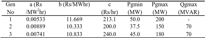
TABLE III GENERATOR DATA
Gen a (Rs b (Rs/MWhr) c Pgmin Pgmax Qgmax No /MW2hr) (Rs/hr) (MW) (MW) (MVAR)
1 0.00533 11.669 213.1 50.0 200 - 2 0.00889 10.333 200.0 37.5 150 70 3 0.00741 10.833 240.0 45.0 180 70
5.1 Case (I) :
In this case the power outputs of three generators are considered as the control variable and OPF is executed to minimize the operating cost given by
n
f(u) = ai Pgi2+bi Pgi +ci (9) i=1
operating cost. Here, the reactive generation of bus 3 is at its maximum both in LP method as well as in the proposed method. The dependent bus voltages are constrained to vary within ±5%.
TABLE IV SOLUTION OF TEST SYSTEM UNDER CASE(I)
Method Pg1 Pg2 Pg3 |v1|sched |v2|sched |v3|sched Loss Cost
(MW) (MW) (MW) (MW) (Rs/hr) Base case 107.9 50 60 1.5 1.0499 1.0429 7.87 3189.4 LP 86.9 59.3 71.0 1.05 1.05 1.0458 7.14 3157.9 PSO 78.98 65.92 72.0 1.05 1.05 1.0644 6.909 3146.2
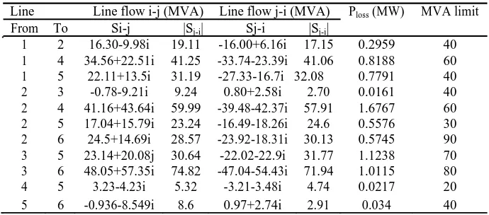
Table -V shows the line flow on the various lines in both the directions obtained from PSO method and their MVA limits. It is observed that line2-4 is at its maximum MVA limit and the losses incurred are also high in the line. While solving using LP method the same line is found to impose binding constraint. From the table it is clear that line flow in all other lines lie well below the limit.
TABLE V LINE FLOWS OF SYSTEM USING PSO UNDER CASE(I)
Line Line flow i-j (MVA) Line flow j-i (MVA) Ploss (MW) MVA limit
From To Si-j |Sj-i| Sj-i |Sj-i|
1 2 16.30-9.98i 19.11 -16.00+6.16i 17.15 0.2959 40 1 4 34.56+22.51i 41.25 -33.74-23.39i 41.06 0.8188 60 1 5 22.11+13.5i 31.19 -27.33-16.7i 32.08 0.7791 40 2 3 -0.78-9.21i 9.24 0.80+2.58i 2.70 0.0161 40 2 4 41.16+43.64i 59.99 -39.48-42.37i 57.91 1.6767 60 2 5 17.04+15.79i 23.24 -16.49-18.26i 24.6 0.5576 30 2 6 24.5+14.69i 28.57 -23.92-18.31i 30.13 0.5745 90 3 5 23.14+20.08j 30.64 -22.02-22.9i 31.77 1.1238 70 3 6 48.05+57.35i 74.82 -47.04-54.43i 71.94 1.0115 80 4 5 3.23-4.23i 5.32 -3.21-3.48i 4.74 0.0217 20 5 6 -0.936-8.549i 8.6 0.97+2.74i 2.91 0.034 40
5.2 Case(II) :
In this case, the power outputs of three generators and its voltages are considered as the control variable and OPF is executed to minimize the operating cost (9) with the following six control variables.
u = [Pg1 Pg2 ...Pgn |U1| |U2| ....|Un| ]
TABLE-VI: SOLUTION OF TEST SYSTEM UNDER CASE(II)
Method Pg1 Pg2 Pg3 |U1|sched |U2|sched |U3|sched Loss Cost
(MW) (MW) (MW) (MW) (Rs/hr) LP 52.23 87.5 77.0 1.05 1.0429 1.0499 6.73 3127.4 PSO 54.60 85.11 77.15 1.05 1.0317 1.0496 6.87 3129.9
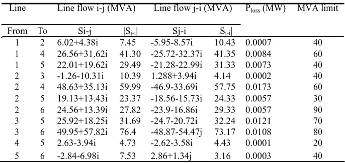
Table -VII shows the line flows for case(ii) obtained from PSO method and their MVA limits. Here, the reactive generation of bus 3 is at its maximum both in LP method as well as in the proposed method.
TABLE -VII : LINE FLOWS OF SYSTEM USING PSO UNDER CASE(II)
Line Line flow i-j (MVA) Line flow j-i (MVA) Ploss (MW) MVA limit
From To Si-j |Sj-i| Sj-i |Sj-i|
1 2 6.02+4.38i 7.45 -5.95-8.57i 10.43 0.0007 40 1 4 26.56+31.62i 41.30 -25.72-32.37i 41.35 0.0084 60 1 5 22.01+19.62i 29.49 -21.28-22.99i 31.33 0.0073 40 2 3 -1.26-10.31i 10.39 1.288+3.94i 4.14 0.0002 40 2 4 48.63+35.13i 59.99 -46.9-33.69i 57.75 0.0173 60 2 5 19.13+13.43i 23.37 -18.56-15.73i 24.33 0.0057 30 2 6 24.56+13.39i 27.82 -23.9-16.86i 29.33 0.0057 90 3 5 25.92+18.25i 31.69 -24.7-20.72i 32.24 0.0121 70 3 6 49.95+57.82i 76.4 -48.87-54.47j 73.17 0.0108 80 4 5 2.63-3.94i 4.73 -2.62-3.58i 4.43 0.0001 20 5 6 -2.84-6.98i 7.53 2.86+1.34j 3.16 0.0003 40
5.3 Case (III) :
In this case the generator voltages of three units are considered as the control variable and OPF is executed to minimize the transmission losses in the systems as given by
Min Ploss(x) => Min Pslack(x) (10)
and u = [|U1| |U2| ...|Un|];
TABLE VIII SOLUTION OF TEST SYSTEM UNDER CASE(III)
Method Pg1 (MW) Pg2 Pg3 |U1|sched |U2|sched |U3|sched Cost Loss
(MW) (MW) (Rs/hr) (MW)
LP 107.743 50 60 1.05 1.0429 1.0499 3187.8 7.7436 PSO 107.712 50 60 1.05 1.0346 1.0436 3187.4 7.7129
TABLE -IX : LINE FLOWS OF TEST SYSTEM USING PSO UNDER CASE(III)
Line Line flow i-j (MVA) Line flow j-i (MVA) Ploss (MW) MVA limit
From To Si-j |Sj-i| Sj-i |Sj-i|
1 2 29.01-7.69i 30.02 -28.22+4.93i 28.65 0.0079 40 1 4 43.35+26.35i 50.72 -42.12-25.57i 49.28 0.0122 60 1 5 35.36+17.13i 39.28 -34.15-18.71i 38.94 0.0121 40 2 3 2.43-7.41i 7.79 -2.42+0.98i 2.61 0.0001 40 2 4 33.49+41.42i 53.26 -32.12-40.71i 51.86 0.0137 60 2 5 15.86+15.53i 22.19 -15.33-17.97i 23.62 0.0053 30 2 6 26.44+15.42i 30.81 -25.76-19.05i 32.04 0.0068 90 3 5 18.65+18.92i 26.57 -17.75-22.05i 28.30 0.0090 70 3 6 43.77+55.46i 70.65 -42.84-52.81i 68.00 0.0094 80 4 5 4.25-3.72i 5.64 -4.21-3.78i 5.66 0.0004 20 5 6 1.429-7.492i 7.63 -1.40+1.87i 2.33 0.0003 40
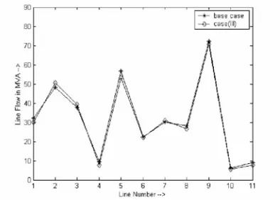
The Line flows in this case are compared with the base case line flows in fig -1. From fig-1 it is concluded that line flows are well controlled if the voltage generating units are controlled for minimizing losses.
Fig. 1. Comparison of line flows in Base case& PSO for test case (III)
6. PARAMETER SELECTION
Maximum number of Generations is found to be 100 for case (I) and (III) where there are only three control variables and it is 500 for test case(II) where the number of control variables are increased to 6 [16].
The acceleration constants ‘c1’ and ‘c2’ are varied in unison from 2 to 8. It is observed that too low value of acceleration (c1=c2=2) results in slow rate of convergence and the global optimum may not be reached within the
specified maximum number of generations. On the other hand, high value of acceleration constants (c1=c2 =8 ) has high
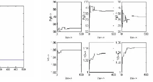
rate of convergence at start but there is a chance of sticking on at the local optimum solution i.e., never converging to global solution. In this paper acceleration constants are chosen to be 5 as optimum. The convergence characteristic of PSO is shown in fig.2 for the test case (ii) with the above specified PSO parameters.
Fig 2: Convergence Characteristic of PSO
for test Case(III)
Fig 2 shows the convergence of control variables for the test case (ii). The figure reveals that the control variables are also converged while the objective function is minimized [17].
VI. CONCLUSION
Now days, as restructuring of power system increases the congestion of power flow in the transmission system, the Optimal Power Flow plays an important role in day to day power system operation and control to maintain system security. Particle Swarm Optimization technique is found to be highly suitable for Optimal Power Flow problem with line flow constraints. It is also assured that the algorithm would function in the same way for large power systems with more number of lines and generating units. The computational results of the sample system reveal that the proposed method is much more efficient and versatile than other methods described.
REFERENCES
[1] Luis S.Vargas, Victor H.Quitana, Anthony Vanneli, "A Tutorial description of an Interior Point method and its applications to Security Constrained Economic Dispatch" IEEE Transactions on Power Systems, Vol-8, No-3, Aug 1993.
[2] Xihui Yan, Victor H.Quintana, "An Efficient Predictor-Corrector Interior Point Algorithm for Security Constrained Economic Dispatch" IEEE Transactions on Power Systems, Vol-12, No-2, May 1997.
[3] Kumaravel, A., Meetei, O.N., "An application of non-uniform cellular automata for efficient cryptography", Indian Journal of Science and Technology, ISSN : 0974-6846, 6(S5) (2013) pp.4560-4566.
[4] Hirotaka Yoshida, Kenichi Kawata, Yoshekasu Fukuyama, Yosuke Nakashini, “ A paricle Swarm Optimization for Reactive Power and Voltage Control Considering Voltage Stability”, IEEE international Conference on Intelligent Syetem Applications to Power Systems, ISAP 99.
[5] Zwe - Lee Gaing, “Particle Swarm Optimization to Slowing the Economic Dispatch Considering the Generating Constraints”, IEEE Trans. on Power Systems, Vol - 18, No -3, Auh 2003
[6] Kumaravel, A., Pradeepa, R., "Efficient molecule reduction for drug design by intelligent search methods", International Journal of Pharma and Bio Sciences, ISSN : 0975-6299, 4(2) (2013) pp.B1023-B1029.
[7] K.Selvi, Dr.N.Ramaraj,S.P.Umaiyal, “Genetic Algorithm Applications to Stochastic Thermal Power Dispatch” Journal of Institution of Engineers (Calcutta), v0l 85, June 2004.
[8] Allen J.Wood, Bruce F.Wollenberg, "Power Generation Operation and Control", John Wiley & Sons Inc. , 1984
[9] Kumaravel, A., Pradeepa, R., "Layered approach for predicting protein subcellular localization in yeast microarray data", Indian Journal of Science and Technology, ISSN : 0974-6846, 6(S5) (2013) pp.4567-4571.
[10] Srinivasan V,Saravanan T, , 2013, Analysis of Harmonic at Educational Division Using C.A. 8332, Middle-East Journal of Scientific Research, ISSN:1990-9233, 16(12), pp.1768-1773
[11] Srinivasan V,Saravanan T, , 2013, Reformation and Market Design of Power Sector, Middle-East Journal of Scientific Research, ISSN:1990-9233, 16(12), pp.1763-1767
[12] Kumaravel, A., Udhayakumarapandian, D.,"Consruction of meta classifiers for apple scab infections", International Journal of Pharma and Bio Sciences, ISSN : 0975-6299, 4(4) (2013) pp.B1207-B1213.
[13] Srinivasan V,Saravanan T, R.Udayakumar, , 2013, Specific Absorption Rate In The Cell Phone User’s Head, Middle-East Journal of Scientific Research, ISSN:1990-9233, 16(12), pp.1748-1750
[14] S.P.Vijayaragavan, B.Karthik, T.V.U.Kiran Kumar and M. Sundar Raj, 2013, Analysis of Chaotic DC-DC Converter Using Wavelet Transform, Middle-East Journal of Scientific Research, ISSN:1990-9233, 16(12), pp.1813-1819
[15] Lydia Caroline M., Vasudevan S., "Growth and characterization of pure and doped bis thiourea zinc acetate: Semiorganic nonlinear optical single crystals", Current Applied Physics, ISSN : 1567-1739, 9(5) (2009) pp. 1054-1061.
[16] S.P.Vijayaragavan, B.Karthik, T.V.U.Kiran Kumar and M. Sundar Raj, 2013, Robotic Surveillance For Patient Care In Hospitals, Middle-East Journal of Scientific Research, ISSN:1990-9233, 6(12), pp.1820-1824