Gram-Schmidt Orthogonalization and Gaussian
Sampling in Structured Lattices
Vadim Lyubashevsky1,2? and Thomas Prest2,3 1
INRIA
2 Ecole Normale Sup´´ erieure
{vadim.lyubashevsky,thomas.prest}@ens.fr 3
Thales Communications & Security
Abstract. A procedure for sampling lattice vectors is at the heart of many lattice constructions, and the algorithm of Klein (SODA 2000) and Gentry, Peikert, Vaikuntanathan (STOC 2008) is currently the one that produces the shortest vectors. But due to the fact that its most time-efficient (quadratic-time) variant requires the storage of the Gram-Schmidt basis, the asymptotic space requirements of this algorithm are the same for general and ideal lattices. The main result of the current work is a series of algorithms that ultimately lead to a sampling proce-dure producing the same outputs as the Klein/GPV one, but requiring only linear-storage when working on lattices used in ideal-lattice cryp-tography. The reduced storage directly leads to a reduction in key-sizes by a factor of Ω(d), and makes cryptographic constructions requiring lattice sampling much more suitable for practical applications.
At the core of our improvements is a new, faster algorithm for computing the Gram-Schmidt orthogonalization of a set of vectors that are related via alinear isometry. In particular, for a linear isometry r :Rd →Rd
which is computable in timeO(d) and ad-dimensional vectorb, our algo-rithm for computing the orthogonalization of (b, r(b), r2(b), . . . , rd−1(b)) usesO(d2) floating point operations. This is in contrast toO(d3) such
op-erations that are required by the standard Gram-Schmidt algorithm. This improvement is directly applicable to bases that appear in ideal-lattice cryptography because those bases exhibit such “isometric structure”. The above-mentioned algorithm improves on a previous one of Gama, Howgrave-Graham, Nguyen (EUROCRYPT 2006) which used different techniques to achieve only a constant-factor speed-up for similar lattice bases. Interestingly, our present ideas can be combined with those from Gama et al. to achieve an even an larger practical speed-up.
We next show how this new Gram-Schmidt algorithm can be applied to-wards lattice sampling in quadratic time using only linear space. The main idea is that rather than pre-computing and storing the Gram-Schmidt vectors, one can compute them “on-the-fly” while running the
?
sampling algorithm. We also rigorously analyze the required arithmetic precision necessary for achieving negligible statistical distance between the outputs of our sampling algorithm and the desired Gaussian distri-bution. The results of our experiments involving NTRU lattices show that the practical performance improvements of our algorithms are as predicted in theory.
1
Introduction
Sampling lattice points is one of the fundamental procedures in lattice cryptog-raphy. It is used in hash-and-sign signatures [GPV08], (hierarchical) identity-based encryption schemes [GPV08,CHKP10,ABB10], standard-model signatures [ABB10,Boy10], attribute-based encryption [BGG+14], and many other con-structions. Being able to output shorter vectors leads to more secure schemes, and the algorithm that produces the currently-shortest samples is the random-ized version of Babai’s nearest-plane algorithm [Bab86] due to Klein [Kle00] and Gentry, Peikert, Vaikuntanathan [GPV08].
The main inefficiency of cryptography based on general lattices is that the key size is usually (at least) quadratic in the security parameter, which is related to the fact that ad-dimensional lattice is generated bydvectors. For security, the lattice dimension is usually taken to be on the order of 512, and this results in keys that are larger than one megabyte in size and unsuitable for most real-world applications. For this reason, all practical implementations of lattice schemes (e.g. [HPS98,LMPR08,LPR13a,DDLL13]) rely on the hardness of problems in ideal lattices [PR06,LM06,LPR13a], which are lattices that correspond to ideals in polynomial rings and can be represented by one or two polynomials.
During its execution, the Klein/GPV algorithm is implicitly computing the Gram-Schmidt orthogonalization of the input basis.1 Since the Gram-Schmidt procedure requires Θ(d3) operations, the Klein/GPV sampler also requires at least this much time. For improving the time-complexity, one can pre-compute and store the Gram-Schmidt basis, which results in a sampling procedure that uses only Θ(d2) operations. The Gram-Schmidt basis requires the storage of
Θ(d2) elements, and so the key size is, as mentioned above, unacceptably large. One may hope that, again, using ideal lattices will decrease the required stor-age. In this case, unfortunately, ideal lattices do not help. The Gram-Schmidt orthogonalization procedure completely destroys the nice structure of ideal lat-tices. So while an ideal lattice basis can be represented by one or two vectors, its Gram-Schmidt basis will havedvectors. Thus theΘ(d2)-operation Klein/GPV algorithm requires as much storage when using ideal lattices as general lattices, and is equally unsuitable for practical purposes. Therefore the only realistic so-lution is to not store the pre-processed Gram-Schmidt basis, which would then allow for the ideal lattice algorithm to be linear-space (since only the original,
1
compact-representation basis needs to be stored), but require at leastΩ(d3) time due to the fact that the Gram-Schmidt basis will need to be computed.
1.1 Our Results
Our main result is an algorithm that computes the Gram-Schmidt basis of certain algebraic lattices usingΘ(d2), instead ofΘ(d3), arithmetic operations. We then show how this new procedure can be combined with the Klein/GPV sampler to achieve a “best-of-both-worlds” result – a sampling algorithm that requires
Θ(d2) operations, which does not require storing a pre-processed Gram-Schmidt basis. In ideal lattice cryptography, this implies being able to have keys that consist of just the compact algebraic basis requiring only linear storage. Not pre-computing the Gram-Schmidt basis of course necessarily slows down our sampling algorithm versus the one where this basis is already stored in memory. But our new orthogonalization algorithm is rather efficient, and so the slowdown is by less than a factor of 5. In case of amortization (i.e. sampling more than one vector at a time), the running time of our new algorithm becomes essentially the same as that of the one requiring the storage of the orthogonalized basis. As a side note, since the Klein/GPV algorithm is just a randomized version of the classic Babai nearest plane algorithm [Bab86], all our improvements apply to the latter as well.
While analyzing the running-time of lattice algorithms, it is very important to not only consider the number of arithmetic operations, but also the arithmetic precision required for the algorithms to be stable. The run-time of algorithms that are not numerically stable may suffer due to the high precision required dur-ing their execution. A second important issue is understanddur-ing how the precision affects the statistical closeness of the distribution of the outputted vectors ver-sus the desired distribution. We rigorously show that in order to have statistical closeness between the output distribution and the desired discrete Gaussian one be at most 2−λ, the required precision of the Gram-Schmidt basis needs to be a little more (in practice, less than a hundred bits) thanλ. We then experimentally show that our new Gram-Schmidt procedure is rather numerically stable, and the intermediate storage is not much more than the final required precision.2 A third issue that also needs to be considered in practice is the space require-ments of the algorithm during run-time. While the stored basis is very short, it could be that the intermediate computations require much larger storage (e.g. if the intermediate computation requires storing the entire Gram-Schmidt ba-sis to a high precision). Our sampling algorithm, however, is rather efficient in this regard because it only requires storing one Gram-Schmidtvector at a time. 2 The reason that we only do experimental analysis of this second part, rather than a
The storage requirement during run-time is therefore less than 64KB for typical dimensions used in cryptographic applications.
Isometries and Ideal Lattices. Interestingly, our improved orthogonaliza-tion algorithm for ideal lattices does not have much to do with their algebraic structure, but rather relies on their implicit geometric properties. The types of bases whose Gram-Schmidt orthogonalization we speed up are those that con-sist of a set of vectors that are related via a linear isometry. In particular, if
H is ad-dimensional Hermitian inner-product space andr:H →H is a linear map that preserves the norm and is computable usingO(d) operations, then we show (both theoretically and via implementations) that orthogonalizing a set of vectors {b, r(b), r2(b). . . , rd−1(b)} can be done using Θ(d2) floating point operations.
We now explain the connection between isometries and ideal lattices. Con-sider the cyclotomic number field, with the usual polynomial addition and mul-tiplication operations,F =Q[X]/hΦm(X)iwhereΦm(X) is themth cyclotomic polynomial (and so it has degree φ(m)). Elements in F can be represented via a canonical embedding3 into
Cφ(m), and in that caseF becomes isomorphic, as
an inner product space, to Rφ(m) where the inner productha,biof a,b∈F is defined as
ha,bi= X
1≤i≤m,gcd(i,m)=1
a(ζi m)·b(ζ
i m),
whereζm∈Cis anmthroot of unity (c.f. [LPR13b, Sections 2.2, 2.5.2]).4
With the above definition of inner product (which is in fact the usual in-ner product over Cφ(m) when elements inF are represented via the canonical embedding), the norm of an elementb∈F is
kbk= s
X
1≤i≤m,gcd(i,m)=1
|b(ζi m)|2. Since all ζi
m, where gcd(i, m) = 1, are roots of Φm(X) and |ζmi | = 1, one can check that for any b ∈ F, kbk = kbXk. Since the function r : F → F
defined as r(b) = bX is linear, it is also an isometry (since it preserves the norm). Furthermore, since F is a field, for any non-zero b∈ F, the elements
b,bX,bX2, . . . ,bXφ(m)−1 are all linearly-independent. When bis an element ofR=Z[X]/hΦm(X)i, the set
{b,bX,bX2, . . . ,bXφ(m)−1}={b, r(b), r2(b), . . . , rφ(m)−1(b)}
3
The canonical embedding of a polynomialb∈F is a vector in Cφ(m) whose
coeff-cients are the evaluations ofbon each of theφ(m) complex roots ofΦm(X).
4
We point out that the actual computation of the inner product does not require any operations overC. The reason is thatha,bi=P1≤i≤m,gcd(i,m)=1a(ζmi )·b(ζmi) can be rewritten as (Va)TVb=aT
VTVbfor a Vandermonde matrixV with coefficients inC. The matrixVTV, however, is a simpleinteger matrix multiplication by which
can be performed in linear time for most “interesting” cyclotomic polynomials (e.g.
therefore generates the ideal hbi as an additive group. Such bases containing short elements can serve as private keys in cryptographic schemes.5
Paper Organization. In Section 2, we set up the notations and definitions that will be used throughout the paper. In Section 3.1, we describe a simple version of our new algorithm that efficiently orthogonalizes a given set of vectors, and in Section 3.2 we give the full, optimized algorithm. In Section 4, we describe an algorithm that, given the orthogonalization, returns the transformation matrixµ
that converts the set{b, r(b), . . . , r(b)}to{b˜1,b˜2, . . . ,b˜n}. In Section 5, we ex-tend our basic algorithms to those that can more efficiently orthogonalize sets of vectors of the formb1, r(b1), . . . , rn−1(b1),b2, r(b2), . . . , rn−1(b2),b3, r(b3), . . .. These types of sets are the ones that normally occur as secret keys in lattice cryptography. A particular example of such a set is the NTRU lattice, which we discuss in Section 7. In that section, we also give timing comparisons be-tween the exact version of our orthogonalization algorithm (which is analyzed in Section 6), and that of [GHN06], for computing the Gram-Schmidt orthogo-nalization of NTRU lattices. Since the two algorithms use different techniques to achieve speed-ups, we demonstrate that the two improvements can comple-ment each other in the form of an even faster algorithm. In Section 8, we show how to implement Babai’s nearest plane algorithm and the Klein/GPV sampling in linear space for lattices whose basis contains vectors that are related via an isometry. In Section 9 we focus on the implementation aspects of our results. In particular, we analyze the required precision to insure the correct functionality of our sampling algorithm.
1.2 Related Work
Computing faster orthogonalization for vectors that are somehow related has been considered in the past. For example, Sweet [Swe84] demonstrated an algo-rithm that orthogonalizes d×dToeplitz matrices using O(d2) operations. This is the same linear-time speed-up as for our algorithm, but for a different class of structured matrices.6 The techniques in that paper seem to be rather different
5
Normally, the bases used in schemes have slightly different forms, such as consisting of a concatenation of elements from R, or being formed by several elements inR. Such bases still contain large components that are related via an isometry, and we discuss this in more detail in Section 7.
6
One may imagine that it may be possible to somehow adapt the results of [Swe84] to the orthogonalization of bases of ideal lattices. The idea would be to embed elements ofF =Q[X]/hΦm(X)iinto C=Q[X]/hXm−1i and then try to use the
fact that in the coefficient representation, the elementsb,bX,bX2, . . .inCform a Toeplitz matrix. One would have to also take care to make sure that the norm inF
than in ours – [Swe84] works with the concrete representation of Toeplitz ma-trices, whereas we only rely on the abstract geometric properties of isometries.
For the special case of NTRU lattices, Gama, Howgrave-Graham, and Nguyen [GHN06] devised algorithms that take advantage of a structure of NTRU bases called symplecticity. This allows them to be faster (by a constant factor) than standard Gram-Schmidt orthogonalization when performing orthogonalization in exact arithmetic. We adapt our algorithms for the same application and they outperform those from [GHN06]. And since our algorithm and that of [GHN06] relies on different ideas, it turns out that we can combine the two techniques to achieve a greater overall improvement (see Figure 1 in Section 7).
2
Preliminaries
2.1 Notations
Through the paper, we will be working over ad-dimensional inner product space
H (usually H =Rd or
Cd), withh·,·i andk · k being a scalar product and the
associated norm overH. Except when stated otherwise, vectors will be written in bold, matrices and bases in capital bold, and scalars in non-bold letters.
B={b1, ...,bn}will be either an ordered set of independent vectors, also called basis, or then×dmatrix whose rows are thebi. We denoteBk=Span(b1, ...,bk) to be the vector space spanned by the vectorsb1, ...,bk.
Definition 1. A linear isometry is a linear map r:H →H such that for any
x,y∈H :
hr(x), r(y)i=hx,yi,
or equivalently
kxk=kr(x)k.
For conciseness, we will sometimes say isometry instead of linear isometry. Since the dimension of H is finite, it is immediate that r is invertible. We will be assuming throughout the work that bothr andr−1are computable in time O(d).
Definition 2. Let x ∈ H, and F be a subspace of H. Then Proj(x, F), the projection ofxoverF, is the unique vectory∈F such thatkx−yk= min
z∈Fkx−zk
Proposition 1. Let rbe an isometry and andF be a subspace of H. Then : 1. x⊥F⇒r(x)⊥r(F)
2. r(Proj(x, F)) =Proj(r(x), r(F))
Proof. We prove the two claims separately :
1. Since r preserves the dot product, it also preserves orthogonality between vectors.
2. rpreserves the norm, so
kx−yk= min
z∈Fkx−zk=⇒ kr(x)−r(y)k= minz∈r(F)
kr(x)−zk
2.2 The Gram-Schmidt Orthogonalization
We provide three equivalent definitions of the Gram-Schmidt orthogonalization of an ordered basis. The first one is geometrical, the second one is a mathematical formula, and the third one looks at each vector of the basis as its decomposition over two orthogonal vector spaces. Although the two first definitions are standard and useful for comprehension and computation, the third one is less common and we will mostly use it to prove that a basis is indeed the orthogonalization of another one.
Definition 3. Let the basis B={b1, ...,bn} be an ordered set of vectors inH.
Its Gram-Schmidt orthogonalization (GSO) is the unique basisB˜ ={b˜1, ...,b˜n}
verifying one of these properties :
– ∀k∈J1, nK,b˜k=bk−Proj(bk,Bk−1)
– ∀k∈J1, nK,b˜k=bk− k−1
P
j=1 hbk,b˜ji
kb˜jk2 ˜
bj
– ∀k∈J1, nK,b˜k⊥Bk−1 and(bk−b˜k)∈Bk−1
The basesBandB˜ then satisfy :∀k∈J1, nK,Bk= ˜Bk. For a vectorbk, we will
say thatb˜k is its Gram-Schmidt reduction (GSR).
Algorithm 1 describes the Gram-Schmidt process as it is usually presented.
Algorithm 1GramSchmidt Process(B)
Require: BasisB={b1, ...,bn}
Ensure: Gram-Schmidt reduced basis ˜B={b˜1, ...,b˜n} 1: fori= 1, ..., ndo
2: b˜i←bi
3: forj= 1, ..., i−1do 4: µi,j=
hbi,b˜ji k˜b
jk2
5: ˜bi←b˜i−µi,jb˜j 6: end for
7: end for
8: return B˜ ={b˜1, ...,b˜n}
2.3 The Gram-Schmidt and LQ Decompositions
Definition 4 (Gram-Schmidt Decomposition). Let B be a d×n matrix.
B can be uniquely decomposed as B =µ×B˜, where B˜ is the GSO of B and
µ= (µi,j)16i,j6n is the lower triangular matrix such that
µi,j =
hbi,b˜ji
kb˜jk2 if i > j 1 if i=j
0 otherwise
Notice that the matrixµ is automatically constructed in Algorithm 1 while computing the GSO. This, however, will not be the case in our improved GSO algorithm, and this is why in this paper we will differentiate between GSO and GSD.
We now recall the definition ofLQdecomposition and give its natural relation to theB=µ×B˜ decomposition.
Definition 5 (LQ decomposition). Let B be a square invertible matrix. B
can be decomposed asB=L×Q, whereLis a lower triangular matrix andQis an orthonormal matrix. If we request the diagonal coefficients ofLto be positive, then this decomposition is unique.
Fact 1 Let B be a square invertible matrix, andB =µ×B˜ its GSD. An LQ
decomposition ofBcan be computed in timeO(n2)by taking Q=D−1×B˜ and
L=µ×D, whereD=Diag(kb˜1k, ...,kb˜nk).
2.4 Discrete Gaussians
Discrete Gaussians aren-dimensional Gaussians discretized over some latticeΛ.
Definition 6. The n-dimensional Gaussian function ρσ,c : Rn → (0,1] of
standard deviation σand centercis defined by :
ρσ,c(x)
∆
= 1
(σ√2π)n exp
−kx−ck
2 2σ2
For any latticeΛ⊂Rn,ρ σ,c(Λ)
∆
=P
x∈Λρσ,c(x). Normalizingρσ,c(x)byρσ,c(Λ),
we obtain the probability distribution function of the discrete Gaussian distribu-tionDΛ,σ,c.
Gaussian Sampling was introduced in [Kle00,GPV08] as a technique to sample from discrete Gaussian distributions, and has since found numerous applications in lattice-based cryptography. In [GPV08], it requires a basisBof the lattice Λ
3
Gram-Schmidt Orthogonalization over Isometric Bases
In this section we present our improved isometric Gram-Schmidt algorithm. In Subsect. 3.1, we present a first simple version which we believe is very intuitive to understand, and then present a slightly faster, more involved, version of it in Subsect. 3.2.
Definition 7. Let B={b1, ...,bn} be an ordered basis of a latticeΛ⊆H. We
say thatB is isometric if there exists an isometryrsuch that
∀k∈J2, nK,bk =r(bk−1)
3.1 A Quadratic-Time algorithm
We now describe a simple algorithm that computes the GSO of any isometric basis in timeΘ(nd) (orΘ(n2) whenn=d).
We briefly expose the general idea behind the algorithm before presenting it formally. If ˜bk is the GSR ofbk, then r(˜bk) is almost the GSR of bk+1 : it is orthogonal tob2, ...,bk, but not tob1. However, reducingr(˜bk) with respect to
b1would break its orthogonality tob2, ...,bk, so what we really need to do is to reduce it with respect tob1−Proj(b1, Span(b2...bk)). Indeed, this latter vector is orthogonal to b2, ...,bk, so reducing r(˜bk) with respect to it won’t break the orthogonality of r(˜bk) to b2, ...,bk. Fortunately, b1−Proj(b1, Span(b2...bk)) can itself be updated quickly. Definition 8 and Algorithm 2 formalize this idea.
Definition 8. Let B = {b1, ...,bn} be an ordered basis and k ∈ J1, nK. We
denotevB,k=b1−Proj(b1, r(Bk−1)). WhenBis obvious from the context, we
simply writevk.
Algorithm 2Isometric GSO(B)
Require: BasisB={b1, ...,bn}
Ensure: Gram-Schmidt reduced basis ˜B={b˜1, ...,b˜n} 1: ˜b1 ←b1
2: v1←b1
3: fork= 1, ..., n−1do 4: b˜k+1←r(˜bk)−
hvk,r(˜bk)i kvkk2 vk
5: vk+1←vk−
hvk,r(˜bk)i kb˜
kk2 r(˜bk)
6: end for
7: return B˜ ={b˜1, ...,b˜n}
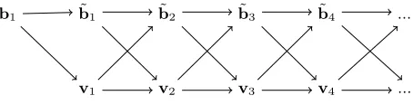
Proposition 2. Let B be an isometric basis with respect tor. Algorithm 2 re-turns the GSO of B. Moreover, if r(v) can be computed in timeO(d) for any
b1 b˜1 b˜2 b˜3 b˜4 ...b˜4
f v1 v2 v3 v4 ...v4
Fig. 1.Computing all the orthogonalized vectors from the first one in Algorithm 2
Proof. We first prove the correctness of the scheme by proving by induction that for everyk∈J1, nK, we have the following :
– vk=b1−Proj(b1, r(Bk−1)) (1)
– b˜k =bk−Proj(bk,Bk−1) (2)
This is trivially true fork= 1. Assuming (1) and (2) are true at stepk, we have:
– Sincevk and ˜bk are already orthogonal tor(Bk−1),vk+1 also is as a linear combination of the two. Butvk+1 is also the orthogonalization ofvk w.r.t.
r(˜bk), so it is orthogonal tor(Bk−1) +Span(r(˜bk)) =r(Bk). On the other hand,b1−vk is inr(Bk−1) sob1−vk+1is inr(Bk). By applying Definition 3, we can conclude that (1) is true fork+ 1.
– The same reasoning holds for ˜bk+1 : it is orthogonal to r(Bk−1) because bothvk andr(˜bk) are. But since it also is orthogonalized w.r.t. vk (in line 4 of the algorithm), it then is orthogonal tor(Bk−1) +Span(vk) =Bk. On the other hand,bk+1−b˜k+1=r(bk−b˜k) +h
r(˜bk),vki
hvk,vki vk is inBk. As before, we can conclude that (2) is true fork+ 1.
Since (2) is verified for anyk∈J1, nK, ˜B is the GSO ofB.
The time complexity of the algorithm is straightforward : assuming additions, subtractions, multiplications and divisions are done in constant time, each scalar product or square norm takes timeO(d). Since there are 3(n−1) norms or scalar products, and 2(n−1) computations ofr(.), the total complexity isO(nd). ut
3.2 Making Isometric GSO Faster
Algorithm 2 is alreadyO(n) times faster than the classical Gram-Schmidt pro-cess. In this subsection, we show that intermediate values are strongly interde-pendent and that this fact can be used to speed up our GSO implementation by about 67%.
Lemma 1. Let B be an isometric basis. For any k in J1, nK, we have the fol-lowing equalities:
– hv1, r(˜bk)i=hvk, r(˜bk)i
When implicit from context, we will denote Ck =hvk, r(˜bk)iand Dk =kb˜kk2.
We have the following recursive formula :
∀k∈J1, n−1K, Dk+1=Dk−
C2 k
Dk
Proof. We prove each of the three equalities separately :
– The equalityhv1, r(˜bk)i=hvk, r(˜bk)iis equivalent to hvk−v1, r(˜bk)i= 0, which is true sincevk−v1=Proj(b1, r(Bk−1)) is in the subspacer(Bk−1) and ˜bk is orthogonal to r(Bk−1)
– The equalitykvkk2 =hvk,v1iis obtained by following the same reasoning as above
– The equality kvkk2 =kb˜kk2 is shown by induction : it is the case for k= 1. By observing that ˜bk+1 is orthogonal to vk from line 4 of Algorithm 2(resp.vk+1is orthogonal tor(bk) from line 5)), we can use the Pythagorean theorem to computekb˜k+1k2andkvk+1k2:
kb˜k+1k2=kb˜kk2−
hvk, r(˜bk)i2
kvkk2
and kvk+1k2=kvkk2−
hvk, r(˜bk)i2
kb˜kk2 At which point we can conclude by induction thatkvk+1k2=kb˜k+1k2, and these equalities also yield us the recursive formulaDk+1=Dk−
C2 k Dk.
u t
This result allows us to speed up further the GSO for isometric bases. At each iteration of the algorithmIsometric GSO, instead of computinghvk, r(˜bk)i,
kb˜kk2 and kvkk2, one only needs to compute hv1, r(˜bk)i, and can instantly compute kb˜kk2 =kvkk2 from previously known values. We choose hv1, r(˜bk)i rather thanhvk, r(˜bk)ibecausev1 has a much smaller bitsize thanvk, resulting in a better complexity in exact arithmetic. Moreover, in the case we use floating-point arithmetic, v1does not introduce any floating-point error, unlikevk. Algorithm 3 sums up these enhancements.
Proposition 3. If B is an isometric basis, then Algorithm 3 returns the GSO of B. Moreover, if we disregard the computational cost of r, then Algorithm 3 performs essentially 3n2 multiplications (resp. additions), whereas Algorithm 2 performs essentially 5n2 multiplications (resp. additions).
Proof. For the correctness of Algorithm 3, one only needs to show that at each step,Ck =hvk, r(˜bk)iandDk =kb˜kk2 =kvkk2. The first and third equalities are given by lemma 1, and the second one by induction : assuming thatCk, Dk are correct,Dk+1 is correct, once again from lemma 1.
Algorithm 3Faster Isometric GSO(B)
Require: BasisB={b1, ...,bn}
Ensure: Gram-Schmidt reduced basis ˜B={b˜1, ...,b˜n}(, (Ck)16k<n,(Dk)16k<n) 1: ˜b1 ←b1
2: v1←b1
3: C1← hv1, r(˜b1)i
4: D1← kb1k2
5: fork= 1, ..., n−1do 6: b˜k+1←r(˜bk)−DCk
kvk
7: vk+1←vk−DCk
kr(˜bk)
8: Ck+1← hv1, r(˜bk+1)i
9: Dk+1←Dk− C2
k
Dk
10: end for
4
Gram-Schmidt Decomposition over Isometric Bases
In this section, we show that the computation of the matrix µfrom the Gram-Schmidt decomposition (or GSD, see Definition 4) can be sped up by a O(n) factor in the case of isometric matrices by using tricks similar to those which led to the speeding-up of GSO. The proof of the following theorem explains how to compute the GSD of an isometric basis/matrix in quadratic time.
Theorem 2. LetB= (b1, ...,bn)be an isometric basis andB˜ = (˜b1, ...,b˜n)its
GSO. For the sake of simplicity, we identify the basis B (resp. B˜) to the (not necessarily square) matrix which rows are the vectors of the basis. Assume we already have B and B˜, along with the values Cj =hvj, r(˜bj)i, Dj =kb˜jk2 for 16j < n. Then the matrix µassociated to B can be computed in time O(n2). Proof. For 1 6 i < j 6 n, let Xi,j = hbi,b˜ji and Yi,j = hr(bi),vji. All the nontrivial values of µi,j (that is, the values µi,j for 1 6 j < i 6 n) can be expressed as µi,j=
Xi,j
Dj . The valuesXi,j, Yi,j satisfy these recursive formulae: (
Xi+1,j+1=Xi,j− Cj DjYi,j
Yi,j+1=Yi,j− Cj DjXi,j
These formulae allow us to compute all the values ofXi,j, Yi,jfrom the 2(n−1) valuesXi,1, Yi,1. Once all of these values are computed, one can simply obtain theµi,j from theXi,j. Algorithm 4 puts this idea into practice.
The idea of this algorithm is somewhat similar to the one behind Algorithms 2 and 3: the only values that we really need to compute are theXi,j’s, but in order to do that efficiently we resort to a mutual recursion involving theYi,j’s.
The time complexity is straightforward. Each Xi,j, Yi,j takes time O(1) to be computed, except for 2nof them which need timeO(n) each. So the overall
Algorithm 4Isometric GSD(B,B˜,(Ci),(Di))
Require: Basis B and its orthogonalization ˜B, valuesCj =hvj, r(˜bj)i, Dj =kb˜jk2 for 16j < n
Ensure: Matrixµ=B×B˜−1
1: Set the diagonal values ofµto 1 and the values above the diagonal to 0 2: fori= 2...ndo{Computing the (Xi,1),(Yi,1)}
3: Xi,1← hbi,b˜1i
4: Yi,1← hr(bi),b1i
5: forj= 2...i−1do 6: Xi,j←Xi−1,j−1−
Cj−1
Dj−1Yi−1,j−1
7: Yi,j←Yi,j−1−
Cj−1
Dj−1Xi,j−1
8: end for 9: end for
10: fori= 2...ndo{Filling out the non-trivial values ofµi,j} 11: forj= 1...i−1do
12: µi,j← Xi,j
Dj
13: end for 14: end for
As an example, the matricesXsteps andXchrono below show, forn= 5, in which order the matricesX, Y are filled. The two matrices use different metrics:
Xchrono displays the chronological order in which the matrices are filled by the algorithm, whereasXstepsdisplay the minimal depth of the computational tree necessary in order to compute anXi,j(resp.Yi,j). If a box contains×, it means that the corresponding value is trivial (see step 1 of the algorithm).
Xsteps=
× × × × ×
1 × × × ×
1 2 × × ×
1 2 3 × ×
1 2 3 4 ×
Xchrono=
× × × × ×
1 × × × ×
2 3 × × ×
4 5 6 × ×
7 8 9 10×
As Xchrono shows, the algorithm fills the matrices X, Y row after row, but if necessary, it could be rewritten in order to fill X, Y column after column, as shown byXsteps.
5
Extending the Results to Block Isometric Bases
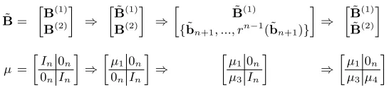
In previous sections, we showed that we can gain a factor O(n) improvement when performing operations such as Gram-Schmidt decomposition on isometric bases. In this section, we show that these results can be extended to block isometric bases, that is bases that are concatenations of isometric bases.
Definition 9. LetB={b1, ...,bkn}be a basis. We say thatBis block isometric
if there existkisometric basesB(1), ...,B(k)such that Bis the concatenation of
The main idea of Algorithm 5 is to use the hypothesis thatr(Span(B(i))) =
Span(B(i)) (which in practice is always verified for ideal lattices) in conjunction with part 2 of Proposition 1 : if ˜bis the GSR ofbw.r.t. a blockB(i), thenr(˜b) will be the GSR ofr(b) w.r.t. that same blockB(i).
Lemma 2. Assume :
– B(1), ...,B(k) are matrices isometric for the same isometry r, and of same
rankn
– ∀i∈J1, k−1K, r(Span(B(i))) =Span(B(i))
Then Algorithm 5 compute the GSO of B ={B(1), ...,B(k)} ={b
1, ...,bkn} in
O(k2nd) elementary operations over the scalars.
Algorithm 5Block GSO(B)
Require: Block isometric basisB={B(1), ...,B(k)}={b1, ...,bkn} Ensure: Gram-Schmidt reduced basis ˜B
1: fori= 0, ..., k−1do 2: b˜ni+1←bni+1
3: forj= 1, ..., nido 4: ˜bni+1←bni+1−
hbni+1,b˜ji kb˜
jk2
˜
bj {Make ˜bni+1 orthogonal to previous vectors}
5: end for 6: B˜(i+1)← {b
ni+1, r(bni+1), ..., rn−1(bni+1)}
7: B˜(i+1)←Faster Isometric GSO( ˜B(i+1)) 8: end for
Proof. We prove correctness by showing inductively that at the end of each iterationiof the outer loop, then(i+ 1) first vectors ˜b1, ...,b˜n(i+1)are the GSO of ˜b1, ...,b˜n(i+1) :
– Fori= 0, this is the case since ˜B(1) is simply the GSO of B(i)
– If it is verified until step i−1, then at step i the vector ˜bni+1 computed in lines 2-5 of the algorithm is exactly the GSR ofbni+1. Its rotations are orthogonal to the vectors of the previous blocks because r preserves the dot product and∀i, r(Span(B(i))) = Span(B(i)), and one can verify that
bni+j−rj−1(˜bni+1) ∈ Span{B˜(1)...B˜(i−1)}, so rj−1(˜bni+1) is exactly the orthogonalization ofbni+j w.r.t.b1, ...,b˜ni. The basis computed at line 6 is isometric, so applyingFaster Isometric GSOeffectively orthogonalize it. We now study the complexity of algorithm 5. At each iterationiof the algorithm, the orthogonalization of bni+1 w.r.t. previous vectors (steps 3 to 5) take time
O(nid), and steps 6-7 take time O(nd). So the total complexity is O(k2nd), gaining a factor n when compared to the complexity O((kn)2d) of the naive
Gram-Schmidt orthogonalisation. ut
˜ B=
B(1) B(2)
⇒ ˜
B(1) B(2)
⇒
˜
B(1)
{b˜n+1, ..., rn−1(˜bn+1)}
⇒ ˜
B(1) ˜ B(2)
µ =
In0n 0nIn
⇒
µ1 0n 0nIn
⇒
µ10n
µ3In
⇒
µ10n
µ3µ4
Fig. 2. Computing the GSD of a two-block isometric basis. ˜B and µ always satisfy
µ×B˜ =B
6
GSO and GSD in Exact Arithmetic
Generally, GSO and GSD are performed over real bases, so the standard way of implementing it is by using floating-point arithmetic. However, this can result in rounding errors: several books and articles discuss this problem with a good introduction being [Hig02].
When the input vectors are in Zd, as it is very often the case in lattice-based cryptography, then the GSD can be performed using only exact arithmetic overQ. Moreover, some algorithms such as the original LLL algorithm [LLL82] explicitely perform exact GSD.
However, this gain in precision comes at the cost of reduced efficiency: when an integer basis undergoes GSO, the reduced vectors’ bitsize quickly escalates in the dimension of the basis and of the underlying space. This phenomenom is calledcoefficient explosion and impacts the spaceand computational cost of GSD. In this section, we adapt Algorithms 3 and 4 to the exact arithmetic setting and show that we still gain a O(d) factor compared to classical GSO/GSD. Moreover, our adapted algorithms completely avoid rational arithmetic.
Through this section, we make an additional “niceness” assumption over the isometryr, namely we suppose that it maps integer vectors into integer vectors:
∀b∈Zd, r(b)∈Zd.
6.1 GSO in Exact Arithmetic
Definition 10. Let B = (bj)16j6n be an isometric basis, and for j ∈ J1, nK,
˜
bj,vj, Cj, Dj be defined as in Section 3. We then define, ∀i, j ∈ J1, nK, the
following values:
• λj,j =Q16k6jkb˜kk2
• db˜ j=λj−1,j−1b˜j
• cj=λj−1,j−1Cj
• λi,j=µi,jλj,j
• dvj =λj−1,j−1vj
• dj =λj−1,j−1Dj
Proposition 4. Using notations of Definition 10,∀i, j∈J1, nK, we have:
1. λi,j∈Z
2. db˜ j,dvj ∈Zd
Proof. Proofs for assertions 1 and 2 can be found per example in [Gal12, chapter 17, theorem 17.3.2]. As for assertion 3, dj =λj,j and cj =hv1, r( ˜dbj)i, where
v1 andr( ˜dbj) are inZd. ut
With these results in hand, we can now devise an integer version of Algo-rithm 3. Instead of outputting rational values, AlgoAlgo-rithm 6 outputs only inte-gers and integer vectors, and one can then retrieve any vector ˜bk by computing ˜
bk = √1 dk−1
˜
dbk. Algorithm 6 uses no rational number and all the internal op-erations, including exact divisions in steps 6,7 and 9, output integer values. The following lemma shows that in the case we use exact arithmetic, Algorithm 6 is still at least O(n) faster than standard GSO.
Algorithm 6Integer Isometric GSO(B)
Require: BasisB={b1, ...,bn}
Ensure: ( ˜dbk,dvk, ck, dk)k=1...nas defined in Definition 10 1: db˜1←b1
2: dv1←b1
3: c1← hr(˜b1),dv1i
4: d1← kb1k2
5: fork= 1, ..., n−1do 6: db˜k+1←
h
dkr( ˜dbk)−ckdvk
i /dk−1
7: dvk+1← h
dkdvk−ckr( ˜dbk)
i /dk−1
8: ck+1← hv1, r( ˜dbk+1)i
9: dk+1←
d2 k−c2k
dk−1
10: end for
Lemma 3. Let B ={b1, ...,bn} ∈(Zd)n be an integral isometric basis, |B|=
max
k=1...n(kbkk)andM(X)denote the time complexity for multiplying two integers
of at most X bits. Suppose the isometry r associated to B can be computed in time and space linear to the size of the input. Then Algorithm 6 performs in timeO(dnM(nlog|B|)).
Proof. By definition,dk =Q16i6kkb˜ik2 so |dk| 6|B|2k. Moreover, |Ck| < Dk implies |ck| < dk and therefore ck, dk both have bitsizes O(klog|B|). On the other hand, ˜dbk (resp.dvk) has its norm less than |B|2k−1 so the four scalar-vectors products performed on steps 6,7 have complexity O(dM(klog|B|)), as well as the two divisions of vectors by scalars (we recall that euclidean division of
X bit numbers can be performed in timeO(M(X))). Overall, each iterationkof theforloop takes timeO(dM(klog|B|)), so the total complexity of Algorithm 6 isO(dnM(nlog|B|)).
6.2 GSD in Exact Arithmetic
The isometric GSD can also naturally be converted into an efficient, “rational-free” version. Let xi,j
∆
= λj−1Xi,j = hbi,db˜ ji ∈ Z and yi,j ∆
= λj−1Yi,j =
hr(bi),dvji ∈Z. The relations
(
Xi+1,j+1=Xi,j− Cj DjYi,j
Yi,j+1=Yi,j− Cj DjXi,j
then become
(
xi+1,j+1=
djxi,j−cjyi,j dj−1
yi,j+1=
djyi,j−cjxi,j dj−1
The xi,j’s actually are the λi,j’s, but in Algorithm 7 we continue to writexi,j since it highlights the natural transformation of Algorithm 4 to Algorithm 7.
Algorithm 7Integer Isometric GSD(B,(ck, dk)k=1...n)
Require: BasisBand the values (ck, dk)k=1...n Ensure: xi,j’s,yi,j’s as defined above
1: fori= 2...ndo{Computing the (xi,1),(yi,1)}
2: xi,1← hbi,b˜1i
3: yi,1← hr(bi),b1i
4: forj= 2...i−1do
5: xi,j←[dj−1xi−1,j−1−cj−1yi−1,j−1]/dj−2
6: yi,j←[dj−1yi,j−1−cj−1xi,j−1]/dj−2
7: end for 8: end for
Lemma 4. Following the notations of Lemma 3, the time complexity of Algo-rithm 7 isO(n2M(nlog|B|) +ndM(log|B|)).
Proof. The costliest operations of Algorithm 7 are either the 2(n−1) dot prod-ucts in steps 2 and 3, which cost O(dM(log|B|)) each, or the essentially 3n2
multiplications and divisions made at steps 5 and 6, which costO(M(jlog|B|))
each. Summing these costs yields the result. ut
7
NTRU Lattices
NTRU lattices are a special class of lattices widely used in cryptography, because their ideal structure allows a gain of a factorn both in time and space when performing usual operations over lattices. This results in efficient and compact cryptosystems (e.g. [HPS98,LTV12,DDLL13]).
Definition 11. Let N, q ∈ N∗ and f, g, F, G ∈ ZN[x] such that f G−gF = q mod (xN + 1). The NTRU lattice generated byf, g, F, G is the lattice generated by the rows of the block matrix
A(f) A(g)
A(F)A(G)
WhereA(p)is the N×N matrix which i-th row is the coefficients ofxi−1·p(x) mod (xN + 1).
In [GHN06], Gama et al. considered exact GSD of NTRU bases. They showed that these lattices verify an algebraic property called symplecticity, which allows them to compute the exact GSD faster than with the standard algorithm, using [GHN06, Corollary 1].
But in addition to beingq-symplectic, NTRU bases are also block isometric. So we devised an algorithm to compute the exact GSD of a NTRU basis, by combining three strategies:
– use Algorithms 6 and 7 in order to avoid rational arithmetic (as in [Gal12] and [GHN06])
– use the GSO/GSD strategies for isometric bases detailed in Section 5
– use [GHN06, Corollary 1] to compute only one half of the GSO and get the other for free
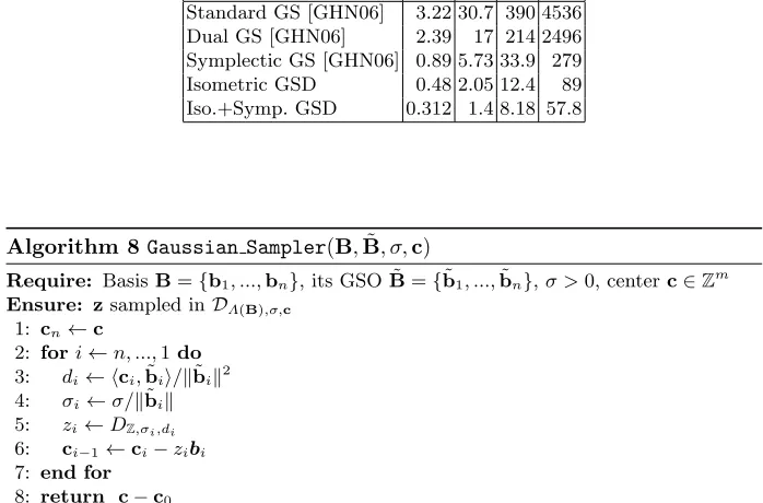
We compared our exact reduction algorithm with the ones from [GHN06]. It turns out that our algorithm is faster, both theoretically and in practice, despite computing more information: it provides ˜B and µ, whereas the algorithms in [GHN06] only provide µ. The timings are summarized in Table 1 and the full implementation can be found athttps://github.com/tprest/Fast-GSD.
8
Reversibility and Application to Linear-Storage
Gaussian Sampling
Gaussian Sampling [Kle00,GPV08] is a cornerstone of lattice cryptography. It can either serve to find approximately close lattice points close to a vector [Kle00], or to sample a lattice point close to a target point without leaking any information about the basis used [GPV08]. We recall the definition of the Gaussian Sampler:
Table 1.Timings for Gram-Schmidt over NTRU bases, in seconds. The implementa-tion was done onSage 5.3. Timings were performed on an Intel Core i5-3210M laptop with a 2.5GHz CPU and 6GB RAM. Isometric GSD is “standard” GSD for block isometric bases, whereas Iso.+Symp. GSD takes into account the observations from [GHN06].
Dimensionn= 2N 128 256 512 1024 Standard GS [GHN06] 3.22 30.7 390 4536 Dual GS [GHN06] 2.39 17 214 2496 Symplectic GS [GHN06] 0.89 5.73 33.9 279 Isometric GSD 0.48 2.05 12.4 89 Iso.+Symp. GSD 0.312 1.4 8.18 57.8
Algorithm 8Gaussian Sampler(B,B˜, σ,c)
Require: BasisB={b1, ...,bn}, its GSO ˜B={b˜1, ...,b˜n},σ >0, centerc∈Zm
Ensure: zsampled inDΛ(B),σ,c 1: cn←c
2: fori←n, ...,1do 3: di← hci,b˜ii/kb˜ik2 4: σi←σ/kb˜ik 5: zi←DZ,σi,di
6: ci−1←ci−zibi 7: end for
8: return c−c0
not the case for the reduced basis ˜B, which needs nvectors. This can quickly impede the practicality of the Gaussian Sampler: for example, for n= 1024 (a typical dimension for cryptographic lattices), if ˜B is stored using 128 bits of precision, the bitsize of ˜Bthen exceeds 128 Mbits.
Our algorithm allows to overcome this problem by computing the reduced basis ˜B on-the-fly. An obstacle is that Gaussian Sampling needs the vectors of
˜
B in reverse order, so a straightforward use of Algorithm 2 or 3 does not solve the problem since it provides the basis in direct order. Fortunately, as Fig. 1 suggests, Algorithms 2 and 3 can be “reversed” in the sense that provided with the last vector ˜bn of the basis ˜Band a few extra pieces of information, one can compute ˜bn−1, ...,b˜1 on-the-fly.
Definition 12. For a basisB, we denote, for anyi∈J1;n−1K,Ci=hvi, r(˜bi)i
andDi =kb˜ik2. We also defineHi=1−(C1 i/Di)2 =
Di
Di+1 andIi=
Ci/Di 1−(Ci/Di)2 = Ci
Algorithm 9Compact Gaussian Sampler(B,B˜, σ,c,b˜n,vn,H,I)
Require: Basis B = {b1, ...,bn}, center c ∈ Zm, precomputed vectors ˜bn,vn, pre-computed values (Hi, Ii)16i<nfrom definition 12
Ensure: zsampled inDΛ(B),σ,c 1: cn←c
2: fori←n, ...,1do 3: di← hci,b˜ii/kb˜ik2 4: σi←σ/kb˜ik 5: zi←DZ,σi,di
6: ci−1←ci−zibi
7: b˜i−1←r−1(Hi−1b˜i+Ii−1vi) 8: vi−1←Ii−1b˜i+Hi−1vi 9: end for
10: return c−c0
Lemma 5. Algorithms 8 and 9 produce the same output when they have the
same inputB andc(assuming the associated precomputed values are correct).
Proof. First, observe that ∀i = 1...n−1, |Ci| < Di, because otherwise Di+1 would be zero andBwould not be a basis. One can see that the ”linear system”
– b˜i+1=r(˜bi)−DCi ivi
– vi+1=vi−CiD ir(˜bi) is invertible :
– b˜i=r−1(Hib˜i+1+Iivi+1)
– vi=Iib˜i+1+Hivi+1
HiandIi are always defined since|Ci|< Di. Therefore, the same way the values
Ci, Di allow to compute ˜bi+1,vi+1 from ˜bi,vi, Hi, Ii allow to compute ˜bi,vi
from ˜bi+1,vi+1. ut
This allows us to perform Gaussian Sampling using O(m) memory space instead ofO(mn) for the classic version. The overhead in time is reasonable :
– Classic Sampler: 2mnadditions, 2mnmultiplications,nsamplings inZ
– Compact Sampler: 4mnadditions , 6mnmultiplications,nsamplings inZ
Therefore, the compact Gaussian Sampler isat most three times slower than the classic one. This is confirmed by experiments summarised in Table??. Moreover, in Algorithm 9, it is possible to sample around severalc’s at the same time: this then makes negligible the overhead induced by the addition (in Algorithm 9) of lines 7 and 8. This time-memory trade-off allows to do Gaussian Sampling fork
targets in spaceO(km) and in timeat most 1 + 2k
times the time required by the classic Gaussian Sampler.
8.1 Analysis of the Space Requirement for the Gaussian Sampler
beforehand), one only needs to store (Hi, Ii,kb˜ik)i=1...nas well as ˜bn,vn. How-ever, it is straightforward to use the relation k˜bi+1k2
kb˜ik2 = 1−
Ci Di
2
to save even more space by just storing the kb˜ik’s and deriving the Hi’s, Ii’s from them. During the execution of Algorithm 9, one also needs to store the current ˜bi,vi. So overall the space requirement of Algorithm 9 is 5n(|log2|+b), where b is less the “number of bits lost” in steps 6, 7 of Algorithm 9: in other words, b
is such that if ˜bn,vn,(kb˜ik)i=1...n are known up to |log2|+b bits, then ˜B is guaranteed to be known up to|log2|bits.
For NTRU lattices, this analysis can be refined: only half of thekb˜ik need to be known, and ˜bn,vn can be determined from b1 = ˜b1 [GHN06, Corollary 1]. Instead of needing to know 3n(|log2|+b) bits beforehand, we just need
n
2(|log2|+b), so the total space requirement is 2.5n(|log2|+b).
9
Precision of the Gaussian Sampler
It is known [GPV08] that for σ big enough, the output f of Algorithm 8 is statistically close to the distribution DΛ(B),σ,c. However, the proof holds only
when B,B˜, σ,c and the valueskb˜ik’s are known exactly. But in practice, one can not afford to do computations with the exact representation of ˜Band of the
kb˜ik’s, as it would be too costly in terms of space and computational resources. Therefore, ˜B and the kb˜ik’s are stored up to some finite precision, and this finite precision introduces errors , δ1 which impact the output distribution of the algorithm. Theorem 3 bounds the statistical distance∆(f, f,δ1) between the output distribution f of the “perfect” algorithm, and the output distribution
f,δ1 of the “imperfect” algorithm.
Theorem 3. Let m, n, q∈N?,B={b
1, ...,bn} ∈Zn×m be a basis of a lattice
Λ⊆Zm,B˜ ={b˜1, ...,b˜n}be the exact GSO ofBandc∈Zm
q . Letδ, , k >0,σ> maxkb˜ik and for anyi= 1...n, letσi =kb˜σ
ik
. Letf,δ1 be the output distribution
of Algorithm 8 ran on input(B,B˜, σ,(kb˜ik)i,c), where the coefficients ofB˜ are
known with absolute precision at least δ1, and the values kb˜ik are known with
relative precision at least. When B˜ and thekb˜ik are known exactly, we simply
refer to the output distribution asf. Let δ3= 2kq
√ m
σ +k
2+ mqδ1k σminikb˜ik
. If δ361/2, then:
∆(f, f,δ1)62n(δ3+ 3e−k 2/2
)
In particular, if we want∆(f, f,δ1)to be less than2−λ for some λ >0, it is
enough that:
δ1, 6
2−λ 2np
λ+ log2np
λ+ log2n+2q √
m
σ +
mq σminikb˜ik
Proof. f is the output distribution of Algorithm 8 executed on exact input (B,B˜, σ,(kb˜ik)i,c), andf,δ1 is the output distribution of Algorithm 8 executed on input (B,B˜0, σ,(kb˜ik0)i,c), where:
– each vector ˜b0
i of ˜B0 is correct up to log2δ1 bits after the comma:
∀i,kb˜i−b˜0ik∞6δ1
– eachkbik0 is correct up to log2bits:
kb˜ik kbik0 −1
6
– sinceσi=k˜bσik, σ0i= σ
k˜bik0, eachσ 0
i is also correct up to log2bits
Letg=f,δ1. Out goal is makef andg fall into the conditions of Lemma 6 for some X, X0, γ, δ5, so that we can get a bound on their statistical distance. Let X = {P
i=1...nzibi|(z1, ..., zn) ∈ Z
n}. Each possible output z = P izibi implicitely defines (d1, ...dn). Let X0 ={z=Pizibi
∀i,|zi−di|6kσi}. From [Lyu12, Lemma 4.4, part 1],f(X\X0), g(X\X0)61−(1−4e−k2/2
)n
64ne−k2/2 . On the other hand, Lemma 10 tells us that for δ4 ≈ 4δ3 + 4e−k
2/2 , ∀z = P
i=1...nzibi∈X and∀i= 1...n:
1−δ46
DZ,σ0 i,d0i(zi)
DZ,σi,di(zi)
61 +δ4 Combining this with f(z) = Q
i=1...n
DZ,σi,di(z) and g(z) = Q
i=1...n
DZ,σ0
i,d0i(z), we have a bounded ratio gf overX0:
∀z∈X0,1−nδ46(1−δ4)n6
g(z)
f(z) 6(1 +δ4)
n= 1 +nδ
4+O(δ42) Takingγ= 4ne−k2/2andδ5=nδ4, we can now apply Lemma 6:
2∆(f, g)6nδ4+ 2γ
u t
The proof of Theorem 3 resorts to several lemmas that can be found in Appendix A.
9.1 Application to NTRU Lattices
We use the formula obtained in Theorem 3 in order to derive concrete bounds in the case of NTRU lattices. In this particular case, m = n, σminkb˜ik > q [GHN06, Corollary 1] and σ > √q (because Q
ikb˜ik = qn/2). We can also reasonably assume that log2n < λ < qn/2, so
, δ1< 2−λ
8n√λqn =⇒ ∆(f, f,δ1)62
−λ
As an example, forn= 1024, q6226andλ
6256, this means that∆(f, f,δ1)6 2−128provided that ˜B(resp. thekb˜ik’s) is known up toλ+ 35 + log
(resp.λ+ 35) bits of precision.
We now use the results from Subsection 8.1 to determine the space require-ments for the parameters as above. Algorithm 9 requires 2.5n(λ+ 35 +b) bits of space. In experiments we launched on NTRU lattices, we always getb630. We will therefore take this value forb.
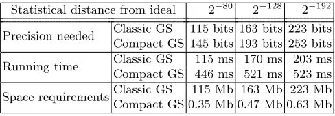
As a test for the practicality of our compact Gaussian Sampler, we imple-mented both the classic and compact Gaussian Samplers and compared their timings and space requirements. As predicted by our computations, the com-pact Gaussian Sampler is no more than thrice slower than the classic one, while having space requirements smaller by between two and three orders of magni-tude. Our results are summarized in Table 2 and the complete implementation can be found on https://github.com/tprest/Compact-Sampler.
Table 2.Timings and space requirements of the classic and compact Gaussian Sam-plers (Classic GS and Compact GS). The implementation was done inC++usingGMP. Timings were performed on an Intel Core i5-3210M laptop with a 2.5GHz CPU and 6GB RAM.
Statistical distance from ideal 2−80 2−128 2−192
Precision needed Classic GS 115 bits 163 bits 223 bits Compact GS 145 bits 193 bits 253 bits
Running time Classic GS 115 ms 170 ms 203 ms Compact GS 446 ms 521 ms 523 ms
Space requirementsClassic GS 115 Mb 163 Mb 223 Mb Compact GS 0.35 Mb 0.47 Mb 0.63 Mb
Acknowledgements
The authors wish to thank Phong Q. Nguyen for helpful comments, as well as the anonymous Eurocrypt’15 reviewers.
References
[ABB10] Shweta Agrawal, Dan Boneh, and Xavier Boyen. Lattice basis delegation in fixed dimension and shorter-ciphertext hierarchical IBE. In Advances in Cryptology - CRYPTO 2010, 30th Annual Cryptology Conference, Santa Barbara, CA, USA, August 15-19, 2010. Proceedings, pages 98–115, 2010. [Bab86] L´aszl´o Babai. On lov´asz’ lattice reduction and the nearest lattice point
[BGG+14] Dan Boneh, Craig Gentry, Sergey Gorbunov, Shai Halevi, Valeria
Niko-laenko, Gil Segev, Vinod Vaikuntanathan, and Dhinakaran Vinayaga-murthy. Fully key-homomorphic encryption, arithmetic circuit ABE and compact garbled circuits. InAdvances in Cryptology - EUROCRYPT 2014 - 33rd Annual International Conference on the Theory and Applications of Cryptographic Techniques, Copenhagen, Denmark, May 11-15, 2014. Pro-ceedings, pages 533–556, 2014.
[Boy10] Xavier Boyen. Lattice mixing and vanishing trapdoors: A framework for fully secure short signatures and more. InPublic Key Cryptography, pages 499–517, 2010.
[CHKP10] David Cash, Dennis Hofheinz, Eike Kiltz, and Chris Peikert. Bonsai trees, or how to delegate a lattice basis. InEUROCRYPT, pages 523–552, 2010. [DDLL13] L´eo Ducas, Alain Durmus, Tancr`ede Lepoint, and Vadim Lyubashevsky.
Lattice signatures and bimodal gaussians. InCRYPTO (1), pages 40–56, 2013.
[Gal12] Steven D. Galbraith. Mathematics of Public Key Cryptography. Cambridge University Press, New York, NY, USA, 1st edition, 2012.
[GHN06] Nicolas Gama, Nick Howgrave-Graham, and Phong Q. Nguyen. Symplectic lattice reduction and ntru. InProceedings of the 24th Annual International Conference on The Theory and Applications of Cryptographic Techniques, EUROCRYPT’06, pages 233–253, Berlin, Heidelberg, 2006. Springer-Verlag. [GPV08] Craig Gentry, Chris Peikert, and Vinod Vaikuntanathan. Trapdoors for hard lattices and new cryptographic constructions. InSTOC, pages 197– 206, 2008.
[Hig02] Nicholas J. Higham. Accuracy and Stability of Numerical Algorithms. So-ciety for Industrial and Applied Mathematics, Philadelphia, PA, USA, 2nd edition, 2002.
[HPS98] Jeffrey Hoffstein, Jill Pipher, and Joseph H. Silverman. NTRU: A ring-based public key cryptosystem. InANTS, pages 267–288, 1998.
[Kle00] Philip N. Klein. Finding the closest lattice vector when it’s unusually close. InSODA, pages 937–941, 2000.
[LLL82] A. K. Lenstra, H. W. Lenstra, and L. Lov´asz. Factoring polynomials with rational coefficients. Mathematische Annalen, 261:515–534, 1982.
[LM06] Vadim Lyubashevsky and Daniele Micciancio. Generalized compact knap-sacks are collision resistant. InICALP (2), pages 144–155, 2006.
[LMPR08] Vadim Lyubashevsky, Daniele Micciancio, Chris Peikert, and Alon Rosen. SWIFFT: A modest proposal for FFT hashing. InFSE, pages 54–72, 2008. [LPR13a] Vadim Lyubashevsky, Chris Peikert, and Oded Regev. On ideal lattices and learning with errors over rings.J. ACM, 60(6):43, 2013. Preliminary version appeared in EUROCRYPT 2010.
[LPR13b] Vadim Lyubashevsky, Chris Peikert, and Oded Regev. A toolkit for ring-lwe cryptography. InEUROCRYPT, pages 35–54, 2013.
[LTV12] Adriana L´opez-Alt, Eran Tromer, and Vinod Vaikuntanathan. On-the-fly multiparty computation on the cloud via multikey fully homomorphic en-cryption. InSTOC, pages 1219–1234, 2012.
[Lyu12] Vadim Lyubashevsky. Lattice signatures without trapdoors. In EURO-CRYPT, pages 738–755, 2012.
[MS07] Vladimir Maz’ya and Gunther Schmidt. Approximate Approximations. AMS, 1st edition, 2007.
[Swe84] D.R. Sweet. Fast toeplitz orthogonalization.Numerische Mathematik, 43:1– 21, 1984.
A
Lemmas used in the Precision Analysis of the Gaussian
Sampler
This section regroups the lemmas used by Theorem 3 in order to bound the sta-tistical distance. We will sometimes resort to approximations such asρd,σ(Z)≈1
in order to simplify computations: indeed,|ρd0,σ(Z)−1|<1.04·10−8σ 2
whenever
σ > √1
2 (see e.g. [MS07, Sect. 1.1]), and that will always be the case through this section. In the same way, we always assumeandδi’s to be very small and will therefore discardδ terms whenever possible. Each time such an approximation is done, it is indicated with signs such asO(·) or≈, and has a negligible impact. More precisely, it never adds “hidden errors” to the result being proven.
The first lemma gives a simple bound on the statistical distance between two distributions f and g which are both in a set X0 with probability 1−γ, and enjoy a relative error bound 1−δ56
g(z)
f(z) 61 +δ5over this setX
0. As one could expect, the statistical distance betweenf and g becomes linear inδ5+γ when
δ5, γ →0.
Lemma 6. Let f, g be two distributions over a set X. Let X0 ⊆ X, δ5, γ >0
such thatP
z∈X\X0f(z), P
z∈X\X0g(z)6γ, and∀z∈X0,1−δ56 g(f(zz))61 +δ5.
Then:
2∆(f, g)62γ+δ5.
Proof. We separate the statistical distance sum into two sums overX0andX\X0: 2∆(f, g)6P
z∈X\X0f(z) + P
z∈X\X0g(z) + P
z∈X0|f(z)−g(z)|
62γ+δ5 P
z∈X0
f(z)
62γ+δ5
u t
The following lemma bounds the error occurring in step 3 of Algorithm 8, when the centerdi is computed. In the floating-point version, the ˜bi are known up to absolute precision δ1 (ie log2δ1 bits after the comma) and their norms
kb˜ik are known up to relative precision (ie log2−log2kb˜ik bits after the comma), whereδ1 andare not necessarily equal.
Lemma 7. Let 0 < δ1, 1, c∈Zmq ,b,b0 ∈ Rm such that kb−b0k∞ 6 δ1
and
kbk kb0k −1
6. Let d = hc,bi kbk2, d0 =
hc,b0i
kb0k2. Then |d−d0| 6δ2, whereδ2 ≈ 2q
√ m kbk +
Proof. d0=hkcb,bk2i+
hc,b0−bi kbk2
kbk2 kb0k2, so
|d0−d|6((1 +)2−1)d+kck1kb0−bk∞
kbk2 (1 +)2
62q √
m
kbk (+O(
2)) + mq
kbk2(δ1+O(δ21))
u t
In the three next lemmas, we study the difference of behaviour between a perfect gaussian over Z of center d and standard deviation σ, and the same gaussian with a slightly perturbed centerd0 and standard deviationσ0. For any center d, DZ,σ,d can be exactly simulated from DZ,σ,d−1 (and reciprocally), so we can suppose w.l.o.g. that d ∈ (−1/2,1/2]. The Lemmas 8, 9 progressively build up to establish in Lemma 10 a bound over the ratio ofDZ,σ,dandDZ,σ0,d0, which are the distributions from which Algorithm 8 samples in step 5 (DZ,σ,din the “perfect” algorithm,DZ,σ0,d0 in the “imperfect” one).
Lemma 8. Let, δ2, k >0, σ, σ0 >1 andd, d0∈(−1/2,1/2]such that|d−d0|6
δ2 and σσ0 −1
6. Let z∈Zsuch that |z−d|6kσ. Then
e−δ3 6 ρσ0,d0(z)
ρσ,d(z) 6
eδ3
where δ3 = δ2σk +(k2 + 1) + O(, δ22, δ2). In particular, if δ3 6 1/2, then
ρσ0,d0(z) ρσ,d(z) −1
62δ3
Proof.
ρσ0,d0(z)
ρσ,d(z)
=ρσ0,d0(z)
ρσ0,d(z)
×ρσ,d0(z)
ρσ,d(z) One one hand,
ρσ,d0(z)
ρσ,d(z)
=e(d0 −d)(2z−d
0+d) 2σ2 , and
(d0−d)(2z−d0+d) 2σ2
6
k
σ(δ2+O(δ
2 2)) On the other hand,
ρσ0,d0(z)
ρσ,d0(z) = σ
σ0 ×e (z−d0)2
2σ2 − (z−d0)2
2σ02
and
(z−d0)2 2σ2 −
(z−d0)2 2σ02
= (z−d 0)2 2σ2
1− σ
2
σ02 6
k2(+O(2)) Combining both inequalities and usingex= 1 +x+O(x2) yield:
ρσ0,d0(z) ρσ,d(z) 6(1 +
k
σ(δ2+O(δ 2
2)) (1 +) 1 +k2(+O(2)
61 + δ2k σ +(k
2+ 1) +O(, δ2 2, δ2)
Lemma 9. Let σ, σ0 > 1 and d, d0 ∈ (−1/2,1/2]. Let k > 0 and Z = {z ∈ Z,|z−d|6kσ}. Suppose ∃δ3∈(0,1/2),∀z∈Z,
ρσ0,d0(z) ρσ,d(z) −1
62δ3. Then: X
z∈Z
|ρσ0,d0(z)−ρσ,d(z)|62δ3+ 4e−k 2/2
Proof. We separate the sum in two sums overZ andZ\Z. For the first sum:
X
z∈Z
|ρσ0,d0(z)−ρσ,d(z)|62δ3 X
z∈Z
|ρσ,d(z)|62δ3(1 + 1.01·10−8)≈2δ3
Now, for the second sum, Lemma 4.4, part 1, from [Lyu12] states that7: For anyk >0,P[|z−d|> kσ;z←DZ,σ,d]62e−k
2/2
Using this lemma, it is straightforward that P
z∈Z\Z
|ρσ,d(z)−ρσ,d0(z)|6 P z∈Z\Z
ρσ,d(z) +ρσ,d(z)
64e−k2/2(ρ
σ,c(Z) +ρσ0,c0(Z))
68e−k2/2δ
3(1 + 1.01·10−8)≈8e−k 2/2
u t
Lemma 10 (Bounded ratio of discrete gaussians over a finite set).Let
σ, σ0 >1 andd, d0 ∈(−1/2,1/2]. Let k >0 and z ∈Z such that|z−d|6kσ.
Suppose∃δ3∈(0,1/2)such that 1−2δ36
ρσ0,d0(z)
ρσ,d(z) 61 + 2δ3. Then:
DZ,σ0,c0(z)
DZ,σ,c(z)
−1 6 δ4
where δ4 = 4δ3+ 4e−k 2/2
+ 4δ2
3+ 8δ3e−k 2/2
. In practice δ3 is small and k is
“somewhat” big, soδ4≈4δ3+ 4e−k 2/2
.
Proof.
|DZ,σ,c(z)−DZ,σ0,c0(z)|=
ρσ,c(z) ρσ,c(Z)−
ρσ0,c0(z) ρσ0,c0(Z) = ρσ,c(z)ρ
σ,c(Z) 1−
ρσ0,c0(z) ρσ,c(z) ×
ρσ,c(Z) ρσ0,c0(Z)
6 ρσ,c(z)ρσ,c(Z)
1−(1 + 2δ3)(1 + 2δ3+ 4e −k2/2)
6DZ,σ,c(z)
4δ3+ 4e−k 2/2
+ 4δ2
3+ 8δ3e−k 2/2
where the penultimate line is obtained by bounding ρσ,c(Z)
ρσ0,c0(Z) via Lemma 9. ut
7