The Mathematical Programming Approach to Applied General Equilibrium Modelling: Notes and Problems

Full text

(1)CENTRE of POLICY STUDIESand the IMPACT PROJECT. Eleventh Floor Menzies Building Monash University Wellington Road CLAYTON Vic 3168 AUSTRALIA Telephone: from overseas: (03) 905 2398, (03) 905 5112 Fax numbers: from overseas: (03) 905 2426, (03)905 5486 e-mail. 61 3 905 2398 or 61 3 905 5112. 61 3 905 2426 or 61 3 905 5486 [email protected]. The Mathematical Programming Approach to Applied General Equilibrium Modelling: Notes and Problems by. Peter B. DIXON Centre of Policy Studies Monash University. Working Paper No. I-50 April 1991. ISSN 1031 9034. ISBN 0 642 10113 2. The Centre of Policy Studies (COPS) is a research centre at Monash University devoted to quantitative analysis of issues relevant to Australian economic policy. The Impact Project is a cooperative venture between the Australian Federal Government and Monash University, La Trobe University, and the Australian National University. During the three years January 1993 to December 1995 COPS and Impact will operate as a single unit at Monash University with the task of constructing a new economy-wide policy model to be known as MONASH. This initiative is supported by the Industry Commission on behalf of the Commonwealth Government, and by several other sponsors. The views expressed herein do not necessarily represent those of any sponsor or government..

(2) ii.

(3) The Mathematical Programming Approach to Applied General Equilibrium Modelling: Notes and Problems by. Peter B. Dixon Centre of Policy Studies Monash University. iii.

(4) iv.

(5) Preface The mathematical programming approach to applied general equilibrium analysis, although no longer the dominant tool, is still useful, from at least two points of view: •. it neatly integrates into an economy-wide framework the microeconomic theory of the behaviour of agents constrained by inequalities; and. •. it provides a useful approach for computing the solutions of some general equilibrium problems not solvable with the current GEMPACK software (see, e.g., Dixon (1991), cited below on p. 16).. The material contained in this paper was meant to be included in our forthcoming graduate-level text (Peter B. D I X O N , B.R. P ARMENTER , Alan A. POWELL and P.J. WILCOXEN , Notes and Problems in Applied General Equilibrium Economics, Amsterdam, NorthHolland), but space limitations led to our reluctant exclusion of it from the text. Publication in the Impact series will mean that those who find the approach in our textbook useful will be able to apply the same method towards mastering mathematical programming in a general equilibrium context.. Peter B. Dixon April 1991. v.

(6) Contents 1 2 3. Preface Introduction Normative versus Positive Analysis Goals, Reading Guide and References Reading guide References. v 1 10 11 12 16. Exercise 1 The implications of technical change in a wine-cloth economy. 18. Section 1 Section 2. What can be produced? What will be produced?. 18 21. Section 3 Section 4. Commodity prices and real wages The effects of a change in production techniques. 21 22. ANSWER TO EXERCISE 1. 30. Exercise 2 A single-consumer linear economy ANSWER TO EXERCISE 2. Exercise 3 The utility possibilities frontier ANSWER TO EXERCISE 3. Exercise 4. A multiple-consumer linear economy ANSWER TO EXERCISE 4. Exercise 5. A linear economy with a utility maximizing consumer ANSWER TO EXERCISE 5. Exercise 6. A linear economy with several utility maximizing consumers ANSWER TO EXERCISE 6. Exercise 7. An introduction to the specialization problem in models of small open economies ANSWER TO EXERCISE 7. Exercise 8. Tariffs, export subsidies and transport costs in a linear model of a small open economy ANSWER TO EXERCISE 8. Exercise 9. A long-run planning model with investment: the snapshot approach ANSWER TO EXERCISE 9. APPENDIX Background Notes on the Theory of Linear Programming A1 The standard linear programming problem A2 Necessary and sufficient conditions for the solution of the standard linear programming problem A3 Basic solutions A4 Proposition on the existence of basic solutions. vi. 32 33. 36 37. 42 44. 46 49. 58 61. 66 69. 74 77. 94 97. 105 105 106 106.

(7) List of Tables E1.1. Current Production Techniques: Input-Output Coefficients. E1.2. Production Techniques after an Improvement in the Technique for Producing Cloth. E1.3 E1.4 E8.1. The Wine-Cloth Economy before and after the Improvement in the Technique for Producing Cloth Occupational Shares in the Workforce Model Solutions under Various Rates of Tariff and Export Subsidy. 18 20 23 27 85. List of Figures 1.1. Utility possibilities set. 6. E1.1 Net annual production possibilities. 19. E1.2 Net annual production possibilities under the initial production techniques. 25. E1.3 Net annual production possibilities after the improvement in the technique for producing cloth. 25. E3.1 Utility possibilities frontiers. 40. E5.1 Indifference curves for a consumer having utility function (E5.6) — (E5.7). 51. E5.2 Indifference map and budget line for the consumer in model (E5.1) — (E5.4), assuming (E5.8) — (E5.10). 53. E5.3 Graphical solution to the problem on the right hand side of (E5.36). 57. E5.4 Indifference map and budget line for the consumer in model (E5.1) — (E5.4), assuming (E5.8) and (E5.10) — (E5.12). 59. E8.1 Cycling in an iterative process. 90. E8.2 Exchange rate solution in a special case of the model (E8.1) — (E8.11). 93. vii.

(8) The Mathematical Programming Approach to Applied General Equilibrium Modelling: Notes and Problems by. Peter B. Dixon Centre of Policy Studies, Monash University 1 Introduction General equilibrium models can often be formulated as mathematical programming (i.e., constrained optimization) problems. To illustrate this approach, we consider a 2-consumer, 2-good, pure trade (no production) model in which the initial endowments are Z1 = . 100.    0 . 0.     100. Z2 = . ,. ,. (1.1). i.e., consumer 1 owns 100 units of good 1 and consumer 2 owns 100 units of good 2. We assume that consumer 1's preferences are described by the utility function U1(C1) = ln(C 11) + ln(C 12). (1.2). where C11 and C12 are his consumption levels for goods 1 and 2 and C 1 is the vector (C 11, C12)′. Similarly, we assume that consumer 2's utility function is U2(C2) = ln(C 21) + ln(C 22) .. (1.3). The problem of solving this model is to find non-negative values for the product prices (denoted by the vector P' ≡ (P1 , P2 )), the consumption vectors (C1 and C2) and the consumer incomes (Y1 and Y2) which jointly satisfy the conditions: Ci maximizes Ui(Ci) subject to P′Ci ≤ Yi , 2. Σ i=1. 1. i=1,2 , (i). 2. Ci –. Σ. Zi ≤ 0 ,. (ii) 1. i=1. Notice that the right hand side of condition (ii) is a 2 ×1 vector of zeros. The right hand side of (iii) is a scalar. Although we use the same symbol, namely 0, the distinction is clear from the context.. 1.

(9) 2. Peter B. Dixon.  P′  . 2. Σ. 2. Σ. Ci–. i=1. Z i. i=1.   . = 0 ,. (iii). and P′Zi = Yi , i=1,2 .. (iv). Condition (i) says that consumers maximize their utilities subject to their budget constraints. Condition (ii) says that demand for each good is less than or equal to supply. This condition combined with (iii) implies that goods in excess supply have zero price. Condition (iv) says that consumers’ incomes are the values of their initial endowments. A price normalization condition must be added if we want to tie down the absolute values for P1 and P2. We also know from Walras' law that either the market clearing condition for one of the goods or the definition of income for one of the consumers could be eliminated. For the present, however, we will leave the model in the form (i) – (iv). Perhaps the most obvious approach to solving general equilibrium models is via excess demand functions. Applying this approach to the model (i) - (iv), we first derive the consumer demand equations from condition (i). Under (1.2) and (1.3) we obtain2 C ij =. 1 Yi 2 Pj. , i, j=1,2 .. (1.4). Next we use (iv) to eliminate the Yi's, i.e., we write (1.4) as C ij =. 1 P′Z i , i,j=1,2 . 2 Pj. (1.5). With the Zis given by (1.1), (1.5) reduces to C 1j=50P C2j=50P. 2. 1/ Pj,j=1 ,2, 2/Pj. ,j=1,2..   . (1.6). If Pj were zero, then under (1.2) and (1.3), demand for good j would be unlimited. Because supply is finite, we may assume (in view of condition (ii)) that neither price is zero..

(10) T he M athematical P rogramming A pproach to A pplied G eneral Equilibrium. 3. On substituting from (1.6) and (1.1) into (ii) we obtain the system of excess demand equations3 50. 50. P1 P1 P1 P2. + 50. + 50. P2 P1. –. 100. =. 0 ,. (1.7). –. 100. =. 0 ,. (1.8). P2 P2. At this stage, we introduce a normalization rule, e.g., P1 = 1 .. (1.9). With this particular rule, (1.7) and (1.8) imply that P2 = 1 . Substituting back into (iv) gives Y1 = Y2 = 100. We complete the solution by substituting into (1.6), obtaining Cij = 50 for all i,j. However, rather than using excess demand functions, here we will deduce solutions to general equilibrium models via mathematical programming problems. In our illustrative model, (i) - (iv), we can use the problem of choosing non-negative values for Cij, i,j=1,2 to maximize 2. Σ. wi Ui (Ci). (1.10). i=1. subject to 2. Σ i=1. 3. 2. Ci –. Σ. Zi ≤ 0 ,. (1.11). i=1. Because neither price is zero, we may assume that condition (ii) is satisfied by equalities..

(11) 4. Peter B. Dixon. where the wis are weights satisfying 2. Σ. wi = 1 .. (1.12). i=1. In problem (1.10) – (1.11), we allocate the available commodities to maximize a weighted average of the utilities of the two consumers. We try to set the weights so that the consumption vectors allocated to the consumers are consistent with their budget constraints. In the present example where (1.1), (1.2) and (1.3) apply, it is intuitively clear that we should set w1 = w2 = 12. Then (1.10) – (1.11) can be written as: C ij ,. choose. i,j=1,2. to maximize 1 2. subject to. {ln(C11) + ln(C12)}. {. + 1 ln(C ) + ln(C ) 21 22 2. }. (1.13). 2. Σ. Cij = 100 ,. j=1,2. .. (1.14) 4. i=1. _ To solve (1.13) – (1.14) we note the if C ij , i,j=1,2, is a solution, then _ _ there exist P1 , P2 ≥ 0 such that _ _ 1/(2Cij) = Pj ,. i=1,2, j=1,2. (1.15). and. 4. We have written the constraints as equalities. The maximization of (1.13) requires that all of the available supplies be used..

(12) T he M athematical P rogramming A pproach to A pplied G eneral Equilibrium 2. Σ. _ Cij = 100 ,. j=1,2. .. 5. (1.16). i=1. (1.15) – (1.16) imply that _ Cij = 50 for i=1,2, j=1,2 and _ Pj = 0.01 for j=1,2 .. (1.17) (1.18). Thus, the solution to the problem (1.13) – (1.14), together with the associated Lagrangian multipliers, has revealed the solution to the model (i) – (iv).5 Why can we solve the model in this way? The main ingredient in the underlying theory is the utility possibilities set (Samuelson (1950)). The utility possibilities set shows all the combinations, (U1, U 2 ), of utility for the two consumers which are possible given their combined resources. Figure1.1 illustrates the utility possibilities set in our example where the utility functions are (1.2) and (1.3) and the resource endowments are given in (1.1). Because there are no market imperfections, externalities or taxes in our model (i) – (iv), we know that solutions will be Pareto optimal. In terms of Figure1.1, the solution to (i) – (iv) will imply utility combinations on the frontier AA. Consequently, one way to solve the model is to search this frontier. There are various methods for obtaining points on the utility possibilities frontier. Problem (1.10) – (1.11), for example, will indicate points on AA. At solutions to (1.10) – (1.11) the utility levels will be at points where the slope of AA is equal to the negative of the ratio of the 1 weights (–w 1 /w 2 ) . (With w1 = w2 = 2 , the solution to (1.10) – (1.11) implies utility levels at B in Figure1.1.) We could. 5. The absolute values (but not the relative values) obtained for the prices differ from those obtained when we worked via the excess demand functions. This is of no importance since our model (i) – (iv) does not determine absolute prices..

(13) 6. Peter B. Dixon. U2. U2 /U1 = 1. 9.210 A. B. U2 = H 2. H2. 1 1 2 U1 + 2 U2. = constant 9.210 U1 A. Figure1.1 Utility possibilities set The utility functions are (1.2) and (1.3) and the combined resources of the two consumers are 100 units of each good, i.e., Z 1 + Z2 = (100, 100). Points on the frontier, AA, are Pareto optimal. At these points, it is impossible to increase the utility of one consumer without reducing the utility of the other. In our example, the equation for the utility possibilities frontier is U2 = 2 ln {100 - exp(U1/2) }. You are asked to derive this equation in Exercise 3(d)..

(14) T he M athematical P rogramming A pproach to A pplied G eneral Equilibrium. 7. also generate points on AA by solving problems of the form: choose nonnegative values for Cij, i,j=1,2 to maximize U1(C11, C12) subject to. 2. Σ and. (1.19). 2. Cij –. i=1. Σ. Zij ≤ 0 ,. j=1,2. (1.20). i=1. U2(C21, C22) _> H2 .. (1.21). In this problem, we allocate the available commodities so as to maximize consumer 1's utility subject to _ consumer 2 achieving a utility level of at least H2 . (If H2 were set at H2 in our example, then problem (1.19) – (1.21) would generate point B in Figure1.1). A third approach to generating points on AA is to solve problems of the form: choose non-negative values for Cij, i,j=1,2 to maximize U1(C11, C12). (1.22). subject to 2. 2. Σ i=1. Cij –. Σ. Zij ≤ 0 ,. j=1,2. (1.23). i=1. and U2(C21, C22) _> β U1(C11, C12) .. (1.24). This time, we maximize consumer 1's utility subject to consumer 2 achieving a utility level of at least β times that of consumer 1. (If β were set at 1 in our example, then problem (1.22) – (1.24) would generate point B in Figure1.1.) The question remains of how we should set the w i s in (1.10) – (1.11) or the H2 in (1.19) – (1.21) or the β in (1.22) – (1.24) so that the particular point generated on the utility possibilities frontier indicates a solution to our model (i) – (iv). How could we have proceeded with problem (1.10) – (1.11), for example, if we had not known the.

(15) 8. Peter B. Dixon 1. 1. appropriate values (w 1 = 2, w2 = 2) for the weights a priori? Except in very simple cases, we must adopt an iterative approach. That is, we must make an initial guess of the appropriate values for the w is; solve problem (1.10) – (1.11); use information from our solution to improve our guess of the wis; re-solve (1.10) – (1.11); improve our guess, etc. If in our numerical example, we had made as an initial guess for the weights (1) 1 (1) 3 (1.25) 6 w1 = 4 , w2 = 4 , then our initial solution to problem (1.10) – (1.11) would have been _ (1) ′ _ (1) ′ (C1 ) = (25, 25) , (C2 ) = (75, 75) , (1.26) 7 with the Lagrangian multipliers being _ ′ ( P(1)) = (0.01, 0.01) .. (1.27). Interpreting the Lagrangian multipliers as commodity prices, this would have implied a value of _ ′ _ ( P(1)) (C(1) 1 ) = 0.5 for consumer 1's expenditure and _ ′ ( P(1)) Z1 = 1.0 for the consumer's income. For consumer 2, expenditure and income would have been 1.5 and 1.0 respectively. These expenditure and income levels are inconsistent with condition (i). To move towards a solution to model (i) – (iv), we would have had to increase w1 relative to w 2 and to re-solve problem (1.10) – (1.11). With a higher value for w 1 /w 2 , problem (1.10) – (1.11) would allocate more consumption to. 6. We use the superscript (s) to denote values of variables in the sth iteration. (1) (1) For example, w1 and w2 are the weights in the first iteration.. 7. (1.26) and (1.27) are easily established by revising (1.15) to read _. 1/(4C1j)=P _. 3/(4C. _. j,j=1,2. _ )=P 2j j,j=1,2..   . (1.28).

(16) T he M athematical P rogramming A pproach to A pplied G eneral Equilibrium. 9. consumer 1 and less to consumer 2. Your exercises and readings will indicate various rules for moving the ws, Hs or βs which have proved effective in practical applications. The final question for this section is: what are the advantages of mathematical programming as a means of solving general equilibrium models compared with working with systems of excess demand functions. Proponents of the mathematical programming approach normally emphasize dimensionality. When we work with the excess demand functions we have n – 1 unknowns where n is the number of commodity prices. (One price can be eliminated via normalization.) In programming problems such as (1.10) – (1.11), (1.19) – (1.21) and (1.22) – (1.24) we have to find values for k – 1 iterative variables where k is the number of consumers. (In problem (1.10) – (1.11), one of the ws can be eliminated via, for example, the normalization rule (1.12).) In many applied models, k (the number of consumers) is small compared to n (the number of commodities). For instance, it is quite common to treat the household sector as if it were composed of a single utilitymaximizing consumer. With k = 1, we can solve models such as (i) – (iv) simply as mathematical programming problems without any iterative search being required. With k = 2, our iterative search involves no more than moving around a one-dimensional frontier such as AA in Figure1.1. Even with larger values of k, say k = 10, it may be easier to search in a (k – 1)-dimensional weight-space (or H-space or β-space) than to derive and solve a system of excess demand functions involving, perhaps, several hundred unknown commodity prices. Of course, in choosing between competing computational approaches, researchers consider many factors apart from dimensionality. For example, are the programming problems which must be solved at each step of the weight-iteration procedure of a computationally simple form? Can they be adequately approximated as linear programming problems? If so, has the local computer centre access to a cheap, user-friendly, linear programming package? If excess demand equations are used, is it necessary that they be excess demand equations for commodities? Would it be preferable to work with excess demand equations for factors? What packages are available for solving systems of non-linear equations? What modifications would be necessary before the available packages could be applied to systems of excess demand functions?.

(17) 10. Peter B. Dixon. 2 Normative Versus Positive Analysis Some of the literature on mathematical programming models blurs the distinction between normative and positive analysis. It is in the hope of helping you to keep the distinction clear that we provide this section. In the previous section we showed how the simple model (i) – (iv) can be solved via mathematical programming. More generally, in the programming approach to economic modelling it is assumed that the vector X of endogenous variables either should be set so as to maximize or will maximize a function f(X, Z). (2.1). g(X, Z) ≤ 0. (2.2). subject to. where (2.2) is a set of constraints containing, for example, demand and supply balances for commodities and factors, and Z is the vector of exogenous variables. The Lagrangian multipliers (also called "shadow prices") associated with the constraints can normally be interpreted as commodity and factor prices. Some models expressed in the form (2.1) – (2.2) are intended to be normative (prescriptive) while others are intended to be positive (descriptive). Because the distinction is important we emphasized, in the previous paragraph, the words "should" (normative models) and "will" (descriptive models). In normative models, positive weights may appear in the objective function (2.1) on variables pertaining to economic growth and equality of income distribution. Alternatively, growth and distribution targets may be included among the constraints. We may also find policy instruments (e.g., taxes, tariffs and government spending) among the choice variables (X). In descriptive models, (1.1) is usually an aggregate utility function formed (explicitly or implicitly) as a weighted sum of the utility functions of individual consumers where the weights reflect relative spending power. Far from giving positive weight to income equality, the objective function in a descriptive model will emphasize the preferences of relatively rich consumers..

(18) T he M athematical P rogramming A pproach to A pplied G eneral Equilibrium. 11. This does not mean, however, that normative analysis is precluded with a descriptive model. It means that analysis is separated into descriptive and normative stages. In the first stage, problem (2.1) – (2.2) is solved with different values for Z. The Z vector in a descriptive model will normally include policy instruments, the computations often being used to describe the effects of adopting different policies under the assumption that the economy operates as if it were maximizing consumer utility subject to resource constraints. In the second stage, the welfare implications of the results of the first stage are evaluated outside the model. This stage will usually be quite informal. The analysts may merely state that he prefers policy A to policy B because he estimates from his model that A will have the more favourable impact on income distribution. Here we will be concerned with descriptive modelling although references are made to some normative planning models. 3 Goals, Reading Guide and References By the time you have completed your reading and finished the exercises, we hope that you will have (1). a facility for expressing general mathematical programming problems;. equilibrium. models. as. (2). a thorough understanding of how general equilibrium models can be solved by a sequence of mathematical programming problems;. (3). a knowledge of how nonlinear mathematical programming problems with convex constraint sets and concave objective functions can be solved as linear programming problems;. (4). an explanation of the overspecialization problem both in intuitive economic terms (what diversifying phenomena are missing) and in terms of the theory of linear programming; and. (5). a familiarity with how investment, restrictions on international trade (tariffs and quotas) and taxes on commodities and factors are handled in the mathematical programming framework.. The reading guide lists some material which will help you to achieve these goals. The readings are referred to in abbreviated form. Full citations are in the reference list. The list also contains other references appearing in the chapter..

(19) 12. Peter B. Dixon. Reading guide *. Begin. Familiar with the theory of mathematical programming including Lagrangian multipliers, the Kuhn-Tucker conditions, sufficiency conditions and the role of convexity?. Yes, but need some revision.. No. Yes. Skim Dixon, Bowles and Kendrick (1980, pp.1-23) and/or Intriligator (1971, chs 1-4 ). This material looks familiar? Ready to go on to something else? Yes. No. A knowledge of the mathematical programming is a prerequisite for fully understanding the material in this chapter. The reading guide on page 3 of Dixon, Bowles and Kendrick (1980) (DBK) suggests various strategies for conquering the relevant material. You may find it useful to work through some of the problems in DBK, e.g., Exercises 1.1, 1.2, 1.3, 1.4, 1.5, 1.8, 1.9 and especially 1.14.. Are you familiar with the theory of linear programming including the existence, duality and complementary slackness theorems? Can you explain linear programming as a special case of nonlinear programming?. Yes. No.

(20) T he M athematical P rogramming A pproach to A pplied G eneral Equilibrium. 13. Reading guide (continued). Yes. No. Read Intriligator (1971, pp.72-89). Pay particular attention to pp.79-86. This reference contains just the right amount of detail for our purposes. We have also provided some brief notes emphasizing the idea of basic solutions in the Appendix. These notes may be sufficient if you need just a quick reminder about linear programming.. The programming problems encountered in applied general equilibrium modeling are usually of a nonlinear variety but with concave objective functions and convex constraint sets. Approximate solutions to these nonlinear programming problems can be obtained by solving suitably chosen linear programming problems. At most computer centres, even very large linear programming problems can be solved cheaply and conveniently. It will therefore be useful for you to know how nonlinear programming problems can be converted into linear programming problems. Read Hadley (1964, pp.104-111) and/or Vajda (1961, pp.218-222).. For an elementary introduction to the idea of solving general equilibrium models by a sequence of mathematical programming problems, read Dixon (1975, pp.1-11). Earlier expositions of the relevant theory are cited there. Of particular importance is Negishi (1960). A recent development is Manne, Chao and Wilson (1980). For straightforward applications of the theory see Dixon (1975, pp.22-39), Ginsburgh and Waelbroeck (1976) and Dixon (1978).. Read Taylor (1975, pp.59-83). This reference covers the theoretical problems of handling investment, taxes and tariffs in the mathematical programming framework. It also contains a section on the overspecialization problem..

(21) 14. Peter B. Dixon. Reading guide (continued). Want to read more about investment? No. Yes. Look at Evans (1972, pp.26-33), Manne (1963), Sandee (1960), Bruno (1967) and Dixon and Vincent (1980, p.349).. The Taylor survey is a little brief on taxes and tariffs. For more information look at Evans (1971) or Evans (1972, pp.18-26), Lage (1970), Dixon (1975, pp.14-22) and Dixon (1978).. Still interested in overspecialization?. No. Yes. Look at Dixon and Butlin (1977, pp.342-344). How do practitioners deal with the overspecialization problem? Refer to Evans (1972, pp.20-23), Lage (1970) and Dixon and Vincent (1980, pp.351-353). Do you consider it is satisfactory to use capacity constraints, fixed import shares and exogenous export flows?.

(22) T he M athematical P rogramming A pproach to A pplied G eneral Equilibrium Reading guide (continued). What are some of the arguments about actual economies that mathematical programming models have been used to support? Refer to the results and conclusions sections of some of the papers you have already read, e.g. Evans (1971), Evans (1972, chs 5-10), Lage (1970), Dixon and Vincent (1980) and Manne (1963). Do you find these conclusions a worthwhile payoff for the effort that has gone into building the models?. Review the list of goals given in this section. Be sure you have reached them by the time you finish your reading and problems.. Exit. * For full citations, see reference list for this chapter.. 15.

(23) 16. Peter B. Dixon. References Baumol, W.J. (1972) Economic Theory and Operations Analysis, 3rd edition, Prentice-Hall. Bruno, M. (1967) "Optimal Patterns of Trade and Development", T h e Review of Economics and Statistics, Vol. 49, November, 545-554. Corden, W.M. (1971) Oxford.. The Theory of Protection, Clarendon Press,. Dixon, P.B. (1975) The Theory of Joint Maximization, North-Holland. Dixon, P.B. (1991) “A General Equilibrium Approach to Public Utility Pricing: Determining Prices for an Urban Water Authority”, Journal of Policy Modeling. Dixon, P.B. (1978) "The Computation of Economic Equilibria: A Joint Maximization Approach", Metroeconomica, Vol. XXIX, 173-185. Dixon, P.B., S. Bowles and D. Kendrick (DBK) (1980) Notes and Problems in Microeconomic Theory, North-Holland. Dixon, P.B. and M.W. Butlin (1977) "Notes on the Evans Model of Protection", Economic Record, Vol. 53 (143), June/September, 337-349. Dixon, P.B. and D.P. Vincent (1980) "Some Economic Implications of Technical Change in Australia to 1990-91: An Illustrative Application of the SNAPSHOT Model", Economic Record, Vol. 56, December, 347-361. Evans, H.D. (1971) "Effects of Protection in a General Equilibrium Framework", Review of Economics and Statistics , Vol. 53, May, 147-156. Evans, H.D. (1972) A General Equilibrium Analysis of Protection, North Holland. Gale, David (1960) The Theory of Linear Economic Models, McGrawHill Book Company. Gayer, A.D., W.W. Rostow and A.J. Schwartz (1953) The Growth and Fluctuation of the British Economy , 1790-1850, 2 volumes, Clarendon, Oxford. Ginsburgh, V. and J. Waelbroeck (1976) "Computational experience with a large general equilibrium model", pp. 257-269 in J. Los and W. Los (eds), Computing Equilibria: How and Why , North-Holland Publishing Company..

(24) T he M athematical P rogramming A pproach to A pplied G eneral Equilibrium. 17. Hadley, G. (1964) Non-Linear and Dynamic Programming, Addison Wesley. Hazari, B.R. (1978) The Pure Theory of International Trade and Distortions, Croom-Helm Publishing Company. Intriligator, M.D. (1971) Mathematical Optimization and Economic Theory, Prentice-Hall. Lage, G.M. (1970) "A Linear Programming Analysis of Tariff Protection", Western Economic Journal, Vol. viii, 167-185. Leontief, W.W. (1978) "Issues of the coming years", Economic Impact, No. 24 (4), 70-76. Lipsey, R.G. and K. Lancaster (1957) "The General Theory of the Second Best", Review of Economic Studies, Vol. 24, February, 11-32. Manne, A.S. (1963) "Key Sectors of the Mexican Economy 1960-1970", pp. 379-400 in A.S. Manne and H.M. Markowitz (eds), Studies in Process Analysis, Wiley. Manne, A.S., Hung-Po Chao and R. Wilson (1980) "Computation of Competitive Equilibria by a Sequence of Linear Programs", Econometrica, Vol. 48 (7), November, 1595-1616. Negishi, T. (1960) "Welfare Economics and the Existence of an Equilibrium for a Competitive Economy", Metroeconomica, Vol. XII, 92-97. Samuelson, P.A. (1950) "Evaluation of Real National Income", Oxford Economic Papers, Vol. 2 (NS), January, 1-29. Sandee, J. (1960) A Long-term Planning Model for India, Asia Publishing House, New York and Statistical Publishing Company, Calcutta. Sauvy, Alfred (1969) General Theory of Population, Weidenfeld and Nicholson, London Taylor, L. (1975) "Theoretical Foundations and Technical Implications", pp. 33-109 in C.R. Blitzer, P.B. Clark and L.Taylor (eds), EconomyWide Models and Development Planning, Oxford University Press. Vajda, S. (1961) Mathematical Programming, Addison-Wesley Publishing Company..

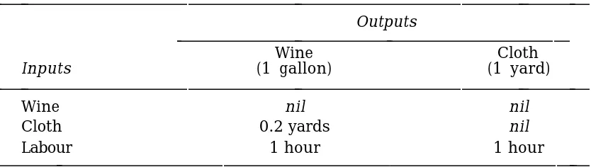
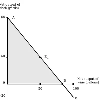
(25) 18. Peter B. Dixon. Exercise 1. The implications of technical change in a wine-cloth economy. This is an easy warm-up exercise. It uses a very elementary model to introduce a few important general equilibrium ideas without algebraic complications. It is organized in four sections. The first describes the net annual production possibilities set, i.e., what can be produced with existing techniques and resources in one year. The second introduces consumer preferences to determine what will be produced. In the third we discuss prices and real wages. In the last section we are ready to derive the implications of a change in production techniques. Table E1.1 Current Production Techniques: Input-Output Coefficients Outputs Inputs. Wine (1 gallon). Cloth (1 yard). Wine Cloth Labour. nil 0.2 yards 1 hour. nil nil 1 hour. Section 1: What can be produced? Consider a society which produces just two products, wine and cloth. The techniques currently in use for the production of these products are described by input-output coefficients in Table E1.1. The output of one gallon of wine requires an input of 0.2 yards of cloth and one hour of labour. The output of one yard of cloth requires an input of just one hour of labour. We assume that the society's resource endowment for a year is 100 labour hours. Given this resource endowment and the production techniques set out in Table E1.1, we can derive the society's net annual production possibilities set. This is shown graphically in Figure E1.1. It can be constructed by doing a few calculations. For example,.

(26) T he M athematical P rogramming A pproach to A pplied G eneral Equilibrium. Net output of cloth (yards) 100. A. 40. E1. Net output of wine (gallons). B. 0 50 -20. 100 D. Figure E1.1 Net annual production possibilities. Given the production techniques in Table E1.1 and a resource endowment of 100 labour hours, our society can produce for final use any combination of wine and cloth shown in the triangle 0AB.. 19.

(27) 20. Peter B. Dixon. if 50 labour hours were devoted to wine and 50 to cloth, then society's net annual output would be 50 gallons and 40 yards. Notice that the gross output of cloth is 50 yards, but that 10 yards are used up in wine production. We have marked the point 50 gallons and 40 yards as E1 in Figure E1.1. Now consider the case in which our society allocates all its resources (100 labour hours) to cloth production. Net annual output would be 100 yards of cloth and no wine (point A in Figure E1.1). On the other hand, if all the labour were devoted to wine, we would end up with 100 gallons, but we would have a deficit of 20 yards of cloth (point D in Figure E1.1). Perhaps the deficit could be made up by drawing on accumulated stocks or through importing. But for simplicity we will assume that there are no accumulated stocks and that there is no international trade. Thus, the net annual production possibilities available to our society are restricted to the shaded area 0AB in Figure E1.1. (a). Can our society produce a net annual output of 40 gallons of wine and 60 yards of cloth?. (b). Can our society produce a net annual output of 40 gallons of wine and 30 yards of cloth?. (c). Consider the production techniques shown in Table E1.2. The only change from those in Table E1.1 is in the labour input coefficient for cloth. Technical progress has taken place which allows a yard of cloth to be produced with only 0.5 hours of labour input rather than one hour. Assume that the society's resource endowment remains at 100 labour hours per year. Can you construct the new net annual production possibilities set?. Table E1.2 Production Techniques after an I mprovement in the Technique for Producing Cloth Wine (1 gallon). Cloth (1 yard). Wine. nil. nil. Cloth. 0.2 yards. nil. 1 hour. 0.5 hours. Labour.

(28) T he M athematical P rogramming A pproach to A pplied G eneral Equilibrium. 21. Section 2: What will be produced? Having constructed society's net annual production possibilities set and illustrated it in Figure E1.1, our next task is to determine which point in the set will be chosen. This will depend on (i) the level of employment and (ii) consumer preferences for wine and cloth. Let us make the assumption that our society achieves full employment, i.e., all of the 100 labour hours are used in production. This contentious assumption is discussed in some detail in the final part of this exercise. If we accept the full employment assumption, then we can restrict our search for the actual net production point to the frontier, AB, of the net annual production possibilities set. It is only on the frontier that we have full employment. Which point will be chosen on the frontier, AB? This will depend on what society wants to consume. Let us consider the simplest possible case by assuming that our society always consumes wine and cloth in fixed proportions: 5 gallons of wine to 4 yards of cloth. In terms of Figure E1.2, consumption will occur somewhere along the line 0C. In fact, in view of our full employment assumption, we can see that net production and consumption of wine and cloth will be 50 gallons and 40 yards (point E1 in Figure E1.2). (d). At E1 how many labour hours will be used in the production of wine? How many will be used in the production of cloth?. (e). Continue to assume that total employment is 100 labour hours and that wine and cloth are consumed in the ratio of 5 gallons to 4 yards. If the production technique for cloth improves to that shown in Table E1.2, what will be the new levels for net production and consumption of wine and cloth? How many labour hours will be used in wine production? How many in cloth production?. Section 3: Commodity prices and real wages At this stage we have come a long way. Starting from a de scription of production techniques and consumer preferences, we have found out what our society will produce and consume, and what.

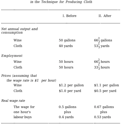
(29) 22. Peter B. Dixon. employment will be in each industry. We can also determine commodity prices and the real hourly wage rate.8 Suppose that the nominal wage rate is $1 per hour. Then under the production techniques shown in Table E1.1, the price of cloth would be $1 per yard. This is because it takes one hour of labour to make a yard of cloth. The price of a gallon of wine would be $1.2, i.e., the cost of one hour of labour plus the cost of 0.2 yards of cloth. The hourly wage ($1) would be just sufficient to buy a commodity bundle containing 0.5 gallons of wine and 0.4 yards of cloth. (f). If the wage rate were $10 per hour, what would be the prices of wine and cloth? Would the wage for an hour's labour still buy a commodity bundle containing 0.5 gallons of wine and 0.4 yards of cloth? In determining the real hourly wage rate, does it make any difference whether we assume the nominal hourly wage is $1 or $10?. (g). Assume that the wage rate is $1 per hour and that the production techniques are those shown in Table E1.2. What will be the prices of wine and cloth? Check that the wage for an hour's labour can now buy a commodity bundle containing 0.67 gallons of wine and 0.53 yards of cloth.. Section 4: The effects of a change in production techniques In Table E1.3 we have listed everything that we have found out about the economy of our wine-cloth society. Column I shows commodity outputs, employment in each industry, commodity prices and the real wage rate in the initial situation (i.e., when the production techniques are those in Table E1.1). Column II shows the corresponding results when the production techniques are those in Table E1.2. By comparing columns I and II, we can see the economywide effects of the improvement in the production technique for cloth. The halving of the labour input coefficient to cloth production has allowed consumption and net production of both wine and cloth to 1 1 increase by 33 3 per cent, real wage rates to increase by 33 3 per cent,. 8. The real hourly wage rate is measured by a quantity of commodities that can be purchased in return for one hour's labour..

(30) T he M athematical P rogramming A pproach to A pplied G eneral Equilibrium. 23. Table E1.3 The Wine-Cloth Economy before and after the Improvement in the Technique for Producing Cloth. I. Before. II. After. Net annual output and consumption 2. Wine. 50 gallons. 66 3 gallons. Cloth. 40 yards. 53 3 yards. Wine. 50 hours. 66 3 hours. Cloth. 50 hours. 33 3 hours. 1. Employment. Prices (assuming that the wage rate is $1 per hour) Wine $1.2 per gallon Cloth. 2 1. $1.1 per gallon. $1.0 per yard. $0.5 per yard. 0.5 gallons. 0.67 gallons. plus. plus. Real wage rate The wage for one hour’s labour buys. 0.4 yards. 0.53 yards. 2. the price of cloth to fall sharply relative to that of wine and 16 3 per cent of the labour force to be reallocated from the cloth industry to the wine industry. This analysis is quite similar to that used by economists concerned with quantifying the effects of technical change in the real world. For example, in their study of the Australian economy, Dixon and Vincent (1980) assembled two tables of input-output coefficients, one.

(31) 24. Peter B. Dixon. showing production techniques as they were in 1971/72 and the other showing the production techniques forecast for 1990/91. 9 They then made some comparisons. Their central computation was designed to answer the following question: how much difference do the projected changes in production techniques make to one's picture of how the economy will be in 1990/91. In terms of Figures E1.2 and E1.3, Dixon and Vincent computed the points E 1 and E2 , where E 1 refers to the levels which would be achieved in 1990/91 for commodity outputs, prices, real wages, etc., if production techniques remained as they were in 1971/72 and E 2 refers to the situation which will emerge if production techniques are consistent with the forecasts. The comparison between E1 and E2 was, therefore, the basis for a discussion of the implications of technical change. Dixon and Vincent had to consider many details which were not included in our wine-cloth economy. They divided the economy into 109 sectors, rather than 2. They included capital, not just labour as a primary factor of production and they divided labour into 9 occupational groups. They considered the role of investment, not just consumption. They allowed for international trade, government expenditure and numerous taxes, tariffs and subsidies. Nevertheless, in essence, their approach consisted of the steps outlined in this exercise: (i) the derivation of alternative net annual production possibilities sets corresponding to alternative assumptions about production techniques, and (ii) the imposition of the full employment assumption and the consideration of consumer preferences leading to the calculation of the net production points. What did Dixon and Vincent conclude from their study? Given the preliminary nature of their work and a number of deficiencies which they were careful to emphasize, they were cautious. They did, however, offer the following:. 9. The forecasts were based on work done by two agencies sponsored by the Australian Government: the Bureau of Industry Economics (BIE) and the IMPACT Project. The BIE selected industries which appeared to be undergoing rapid technical change and asked industry experts to forecast the future input-output coefficients. Where expert opinions were not available, forecasts based on trend projections were prepared by the IMPACT Project..

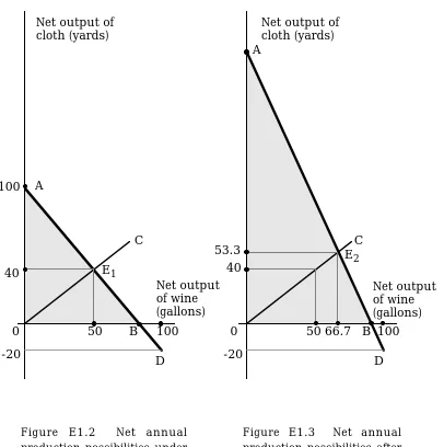
(32) T he M athematical P rogramming A pproach to A pplied G eneral Equilibrium. Net output of cloth (yards). 25. Net output of cloth (yards) A. A. 100. C E1. 40. 0. 50. -20. B. C E2. 53.3 40 Net output of wine (gallons) 100 D. Figure E1.2 Net annual production possibilities under the initial production techniques Apart from the addition of the consumption line, 0C, this figure is the same as Figure E1.1.. Net output of wine (gallons) 50 66.7 B 100. 0 -20. D. Figure E1.3 Net annual production possibilities after the improvement in the technique for producing cloth.

(33) 26. Peter B. Dixon. "The overwhelming impression from Table 4.6 [reproduced here as Table E1.4] is that the occupational composition of the workforce at the 9-order level in 1990/91 is unlikely to be radically different from that in 1971/72 and that it will be determined largely independently of technical change. Certainly, the present simulations do not pinpoint any likely difficulties in the areas of labour mobility and manpower training." [Dixon and Vincent (1980, p. 358)] and "Subject to the qualifications expressed throughout the paper, our results indicate that rapid technical progress is particularly important for the future well-being of those Australian industries which are closely connected with international trade. At the macro level, our results support the view that technical progress is vital for securing increased GDP, increased consumption and higher real wages. Technical progress may also affect macro economic management. In the absence of technical progress, we found that the 'full-employment' level of real wages would decline. Under such conditions, it is difficult to imagine that Australia could achieve even a tolerable approximation to full employment." [Dixon and Vincent (1980, p. 359)] (h). In Table E1.4, you will see references to innovative and Luddite economies. Who were the Luddites?. The calculations by Dixon and Vincent and our own analysis of the wine-cloth economy present technical change in a favourable light. Only its role as a source of increased material welfare is emphasized. But this is not the aspect of technical change which has always been emphasized in popular discussions. Sometimes, the principal concern has been with job replacement. Newspapers frequently report fears expressed by various groups in the community concerning the employment effects of new machines: word-processors, automatic bank tellers, point-of-sale termi nals, vending machines and robots. Let us re-examine our wine-cloth story from the point of view of the employment implications of technical change. The critical assumption in the story is that technical change is not an important determinant of the aggregate level of employment. It is assumed that aggregate employment is 100 labour hours both before and after the improvement in the production technique for cloth. There is no need to assume that.

(34) T he M athematical P rogramming A pproach to A pplied G eneral Equilibrium. 27. Table E1.4 Occupational Shares in the Workforce* I Actual 1971/72 Economy 1.. Professional White Collar. 2.. Skilled White Collar. 12.8. 3.. 26.9. 8.. Semi- and Unskilled White Collar Skilled Blue Collar (Metal & Electrical) Skilled Blue Collar (Building) Skilled Blue Collar (Other) Semi- and Unskilled (Blue Collar) Rural Workers. 9.. Armed Services. 4. 5. 6. 7.. 3.3. 10.9 5.1 2.6 32.0 4.8 1.6 100.0. II 1990/91 Innovative Economy†,#. III 1990/91 Luddite Economy†,#. 3.9 (3.1) 14.3 (2.7) 30.5 (2.9) 9.0 (1.2) 3.9 (0.8) 2.7 (2.5) 30.5 (1.9) 3.6 (0.5) 1.6 (2.2). 4.0 (3.2) 13.6 (2.5) 29.0 (2.6) 9.1 (1.3) 4.1 (1.0) 2.7 (2.5) 30.6 (1.9) 5.1 (2.4) 1.8 (2.7). 100.0 (2.2). 100.0 (2.2). *. Source: Dixon and Vincent (1980, p. 359).. †. Figures in parentheses show annual percentage growth rates over the period 1971/72 to 1990/91. For example, professional white collar employment grows at an average annual rate of 3.1 per cent on the path to the Innovative Economy of 1990/91.. #. Innovative and Luddite were the labels used in Dixon and Vincent (1980). Luddite refers to the calculations for 1990/91 with the input-output coefficients set at their 1971/72 values (the E1 results in Figure E1.2). Innovative refers to the calculations where the input-output coefficients were set at the values forecast for 1990/91 (the E2 results in Figure E1.3). The differences between columns II and III were interpreted as being attributable to technical change..

(35) 28. Peter B. Dixon. employment of 100 labour hours is literally full employment. Perhaps 105. hours of labour are available. Our assumption is that 5 per cent unemployment is just as likely with technical progress as without it.10 This assumption should not be too surprising to readers with some knowledge of conventional macroeconomic theory. That theory stresses demand management, fiscal and monetary policy and the real wage rate in relation to labour productivity as the major determinants of aggregate employment. The rate of technical change rarely rates even a mention. This will not be very reassuring to readers who are sceptical about conventional economic theory. They will want us to spell out the process by which workers, displaced by technical change, will find new jobs. In terms of our wine-cloth economy, the problem is to explain the transition from E1 to E2 (Figures E1.2 and E1.3). Starting at E1, the halving of the labour input coefficient for cloth will mean that only 25 labour hours (rather than 50) are required in the industry. Cloth now will be cheaper and the real incomes of employed workers will expand. These workers will demand more wine and cloth, thus providing employment for the previously displaced workers. This will set us on the happy path to E2. What if capitalists prevent the reduction in the real price of cloth by taking an increase in profits? But don't capitalists consume wine and cloth too? Perhaps not, perhaps capitalists spend on imported luxuries and overseas holidays. But what will the foreigners do with the domestic dollars they receive from the capitalists? They will buy our wine and cloth! But what happens if everyone has had enough wine and cloth? This would be a blissful state — we could simply do less work. Unfortunately a state in which all our material wants are satisfied seems very far away, even in the world's wealthiest countries. What about adjustment problems along the path from E 1 to E2 ? 2 Recall that the shift from E1 to E2 involved the transfer of 16 3 per cent of the labour force out of cloth and into wine. What if the skills required of wine workers differ from those of cloth workers? Then might not. 10. This assumption may be overly generous to the situation with no technical progress. With no technical progress there is unlikely to be scope for increases in real wages without reductions in employment..

(36) T he M athematical P rogramming A pproach to A pplied G eneral Equilibrium. 29. the move from E1 to E2 cause excessive periods of unemployment for surplus cloth workers? Certainly this is a possibility. It is important, therefore, in comparing E 1 and E2 to consider the feasibility of the implied rates of shift of resources between different activities. This is what Dixon and Vincent did in their analysis of the implications of technical change to 1990/91. For example, on examining Table E1.4, they concluded that technical change to 1990/91 could be accommodated without rapid transfers of labour between the nine broadly defined occupational groups. It is possible, however, that technical change to 1990/91 may render redundant certain very specific skills. This does not necessarily imply any serious difficulties. In many countries, workers exhibit a high degree of occupational mobility. We conclude this exercise with two stories about horses, and a question. Horse story number one 11 Maynard, the employer, and his worker, Milton, produce 20 bushels of wheat per year from 5 acres of land. Maynard pays Milton a wage of 10 bushels and retains a profit of 10 bushels for himself. One day, Maynard makes a remarkable technical improvement. He captures and trains a horse. Using the horse, Maynard can produce 20 bushels of wheat per year without Milton's help. Since the horse consumes only 7 bushels of wheat, Maynard sacks Milton and lives happily ever after consuming 13 bushels of wheat per year. But what of poor Milton?. He leaves the farm and starves to. death. Horse story number two 12 Anyone who doesn't believe in the possibility of permanent unemployment arising from technical change should think about what happened to employment prospects for horses at the beginning of this century.. 11. This story is adapted from Sauvy (1969, p. 113).. 12. This story is adapted from Leontief (1978)..

(37) 30 (i). Peter B. Dixon. Have either of these horse stories any relevance to the analysis of the implications of technical change in a modern economy? Both imply the possibility of an unhappy outcome from technical change. What are the key differences in the assumptions underlying our wine-cloth analysis and the assumptions underlying the horse stories?. Answer to Exercise 1 (a) No. In terms of Figure E1.1, the point 40 gallons, 60 yards lies outside the triangle 0AB. Given the production techniques in Table E1.1, it would take a gross output of 40 gallons and 68 yards to achieve a net output of 40 gallons and 60 yards. Thus, 108 hours of labour would be required. Only 100 hours are available. (b) Yes. In terms of Figure E1.1, the point 40 gallons, 30 yards is inside the triangle 0AB. Given the production techniques in Table E1.1, it would take a gross output of 40 gallons and 38 yards to achieve a net output of 40 gallons and 30 yards. Thus, 78 hours of labour would be required. This is available. (c) The new net annual production possibilities set is shown in Figure E1.3 as the triangle 0AB. It can be constructed by considering the net outputs which would emerge as we vary the allocation of labour between the production of our two commodities. For example, if all the 100 labour hours were devoted to cloth production, then we would obtain 200 yards of cloth and no wine. Hence point A in Figure E1.3 is 2 part of the new net annual production possibilities set. If 66 3 hours of 1 labour were devoted to wine and 33 3 to cloth, then net production 2 1 would be 66 3 gallons of wine and 53 3 yards of cloth, point E2 in Figure 1 E1.3. (Notice that the use of 33 3 labour hours in cloth generates a gross 2 1 output of 66 3 yards, but that the wine production uses up 13 3 (= 0.2 × 2 66 3 yards.) If 100 labour hours were devoted to wine production, then we would obtain 100 gallons. There would, however, be a deficit of 20 yards of cloth. (See point D in Figure E1.3.) Because we rule out both international trade and the existence of accumulated stocks, deficits are not possible. Hence the net annual production possibilities are confined to the triangle 0AB in Figure E1.3. Be sure to compare the new net annual production possibilities set with the old one. As can be seen by looking at Figures E1.2 and E1.3, technical progress in the cloth industry leads to an expansion of the possibilities set..

(38) T he M athematical P rogramming A pproach to A pplied G eneral Equilibrium. 31. (d) At E1 , the gross outputs are 50 gallons of wine and 50 yards of cloth. Hence 50 labour hours are used in wine production and 50 in cloth production. (e) In Figure E1.3, the consumption line 0C crosses the frontier of the net annual production possibilities set at E 2 . The levels for net 2 1 production and consumption of wine and cloth are 66 3 gallons and 53 3 2 1 yards. Employment is 66 3 hours in wine and 33 3 hours in cloth. (f) If the wage rate were $10 per hour, the price of cloth would be $10 per yard and the price of wine would be $12 per gallon. The real wage rate would be unaffected by an increase in the wage rate from $1 per hour to $10 per hour. In both cases, the wage for an hour's labour would buy a bundle of commodities containing 0.4 yards of cloth and 0.5 gallons of wine. (g) The price of cloth will be $0.5 per yard and the price of wine will be $1.1 per gallon. At these prices, a commodity bundle containing 0.67 gallons of wine and 0.53 yards of cloth would cost $1, i.e., the wage for one hour of labour would buy a bundle containing 0.67 gallons of wine and 0.53 yards of cloth. (h) The Luddites were organized bands of English workmen who in 1811-12 destroyed stocking frames, steam power looms and shearing machines in various centres of the British textile industry. A popular belief at the time was that these recently introduced labour-saving machines were a cause of low real wages and high unemployment. Luddite activity again broke out in 1816. It is doubtful that technical advances taking place in the British textile industry in the early 19th century had anything to do with the particularly miserable position of British workers in 1811-12 and 1816. In both these years the British economy was in a state of recession arising from poor harvests and high food prices. By blaming technical progress (machines), the workers appear to have misidentified the source of their problems. See, for example, Gayer, Rostow and Schwartz (1953, pp. 135-7). (i) The key differences between the assumptions underlying the horse stories and those underlying the wine-cloth story concern human adaptability to change. In the wine-cloth story, the displaced cloth workers can move into wine production. By contrast, horse story number one depicts the displaced worker, Milton, as having no viable alternative to working for Maynard. One wonders why Milton does not.

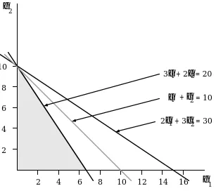
(39) 32. Peter B. Dixon. capture a horse and work some land of his own. Perhaps society has advanced to the stage where all the arable land is occupied. But then it is surprising that Milton does not go to a town and work in an urban occupation. Horse story number two also depicts the possibility of the displaced workers being left with nothing to do, the displaced workers this time being horses. We should note, however, that the horses which lost their jobs at the turn of the century had a very limited range of skills compared with human workers. Exercise 2 A single-consumer linear economy Consider an economy in which an equilibrium is a list of nonnegative vectors and scalars {p, γ, x} satisfying γa≤z+Ax p′( γa–z–Ax)=0 p′A≤0 p′Ax=0. } }. (E 2.1). (E2.2). and p′a = 1 ,. (E2.3). where p is the n × 1 vector of commodity prices, γ is a scalar indicating the number of commodity bundles consumed and x is an m × 1 vector of production activity levels. The exogenous variables are a, the n × 1 vector giving the commodity composition of the consumption bundle; z, the n × 1 vector giving the economy's resource endowments and A, the n × m production technology matrix. The ij th element of A is the input (if negative) or output of good i per unit of activity j. Condition (E2.1) says that demand is less than or equal to supply and that commodities in excess supply have a price of zero. Condition (E2.2) implies that no activity is operated at a positive profit and that activities involving losses are operated at the zero level. Condition (E2.3) fixes the absolute price level. This can be done in other ways. For example, in the last exercise, it was the wage rate which we fixed at one rather than the value of the consumption bundle..

(40) T he M athematical P rogramming A pproach to A pplied G eneral Equilibrium. (a). 33. Assume that 5.  a = 4  0.   ,  . 0. 1.0. 0.0.     z =  0  and A =  –0.2 1.0  .      100   –1.0 –1.0 . What are the equilibrium values for p, γ and x? If we let the three commodities be wine, cloth and labour, then (apart from the choice for the absolute price level) the present model is the same as that in Exercise 1 before the improvement in the technology for making cloth. (b). Assume that a new technique for producing commodity 2 becomes available. The economy's production technology matrix is now 1.0 0.0 –0.1 A =.   –0.2 1.0 1.1   –1.0 –1.0 –1.0.    . Will the new technique be used? (c). In special cases where the numbers of commodities, n, and activities, m, are small, it is possible to solve the model (E2.1) – (E2.3) by elementary graphical and/or algebraic methods. In empirically interesting cases, where n and m may be large, these methods are not adequate. Write down a linear programming problem which would be a suitable vehicle for solving (E2.1) – (E2.3).. Answer to Exercise 2 (a) In this economy, activity 1 is the only method for producing commodity 1 and activity 2 is the only method for producing commodity 2. It is clear, therefore, that both activities must be operated at positive levels. Thus, we can find the equilibrium prices from 1.0. 0.0.   (p1, p2, p3)  –0.2 1.0  = (0,0)    –1.0 –1.0  and.

(41) 34. Peter B. Dixon. 5p1 + 4p2 = 1. .. This gives (p1, p2, p3) = (0.12, 0.10, 0.10). .. Because all prices are positive, we know that the market clearing conditions hold as equalities. Thus, we can determine γ, x 1 and x2 from 5.  γ 4  0. 0. 1.0. 0.0. x.       1  =  0  +  –0.2 1.0    ,          100   –1.0 –1.0   x2 . that is.  x1   x2  γ. –1.0 0.0 5.    0.2 –1.04     1.0 1.0 0 . 0.   =  0     100 . .. (E2.4). On solving equation (E2.4) we obtain x1 = 50,. x2 = 50. and γ = 10. .. (b) Because activity 1 continues to be the only method for producing commodity 1, we may assume that it is still operated at a positive level. If the new activity (activity 3) were also operated at a positive level, the commodity prices would satisfy 1.0. –0.1.   (p1, p2, p3)  –0.2 1.1  = (0, 0)    –1.0 –1.0  and 5p1 + 4p2 = 1. ,. giving (p1, p2, p3) = (0.1193, 0.1009, 0.0991) At these prices, the profit per unit of activity 2 is. .. (E2.5).

(42) T he M athematical P rogramming A pproach to A pplied G eneral Equilibrium. 35. 0.0.    1.0     –1.0. (0.1193, 0.1009, 0.0991). = 0.0018 > 0. .. Thus the prices in (E2.5) are not consistent with (E2.2). We may conclude that the new technique will not be introduced and that the initial equilibrium will not be disturbed. (Just to be safe, check that at the initial prices, the new activity makes non-positive profits.) (c). Consider the problem of choosing non-negative values for γ and x to maximize γ.   . subjectto. (E2.6). γa≤z+Ax. _ _ _ If (γ , x) is a solution to this problem, then there exists p ≥ 0, such that13 _ 1 – p′a = 0 , 14 _ p′A ≤ 0 , _ _ p′Ax = 0 ,. 13. Are you having trouble remembering how to write the conditions for a solution of (E2.6)? The Lagrangian for this problem is L( γ, x, p) = γ – p′(γa – z – Ax) . _. _. _. If (γ , x ) is a solution to (E2.6), then there exists p ≥0 such that ∂L ∂γ. ≤0 ,. γ. ∂L ∂γ. =0 , =0 ,. ∂L ′ [ ∂x ]. ≤0 ,. ∂L ′ [ ∂x ]x. ∂L [ ∂p ]. _> 0 ,. p′ [. ∂L ∂p. ]. =0 , _ _ _. where all these expressions are evaluated at (γ, x, p ). Need more help? Try some of the reading on mathematical programming suggested in the reading guide. 14. _. We assume that γ > 0. Thus we can write this first condition as an equality..

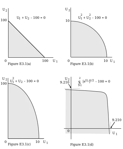
(43) 36. and. Peter B. Dixon. _ _ γ a ≤ z + Ax _ _ _ p ′( γa – z – Ax) = 0. .. Thus solutions for models of the form (E2.1) – (E2.3) may be computed by solving_ linear programming problems of the form (E2.6). The _ solution (γ , x ) to (E2.6), _together with the associated Lagrangian multipliers or dual solution (p ), satisfies the conditions (E2.1) – (E2.3). Exercise 3 The utility possibilities frontier When we move from single-consumer to multiple-consumer models, the utility possibilities frontier becomes a useful concept. As is apparent from subsequent exercises, it is sometimes convenient to solve multiple-consumer models by searching the utility possibilities frontier. In the context of an r-consumer model with a given specification of resource endowments, production technologies and external trading opportunities, the vector of utility levels U ≡ (U1, U2, ...,Ur) is a point on the utility possibilities frontier if and only if U is feasible and _ Ui < Ui for at least one i _ _ _ _ if U ≡ (U 1,...,Ur ) is a feasible utility vector different from U. (U and U are feasible if it is possible to generate the consumption levels required to support them.) In some cases, we can describe the utility possibilities frontier by an equation of the form (E3.1) f(U1,U2, ...,Ur) = 0 where (U1,...,Ur) is a point on the utility possibilities frontier if and only if it satisfies (E3.1). (a). Consider a two-consumer, two-commodity pure exchange model (no production) where the utility functions for the two consumers are 1/2. Ui = (C i1). 1/2. (C i2). ,. i =1,2. (E3.2). and where C ij is the consumption of good j by consumer i. Assume that the consumers' endowment vectors are.

(44) T he M athematical P rogramming A pproach to A pplied G eneral Equilibrium. 37. Z′1 = (100, 0) and. Z′2 = (0, 100). .. Derive the equation for the utility possibilities frontier and provide a sketch of the utility possibilities set. (b). Answer question (a) with (E3.2) replaced by Ui = (C i1). (c). 1/4. (C i2). 1/4. ,. i=1,2. .. (E3.3). Answer question (a) with (E3.2) replaced by U1 = (C 11). 1/4. 1/4. (C 12). (E3.4). and 1/2. U2 = (C 21) (d). (C 22). 1/2. .. (E3.5). Answer question (a) with (E3.2) replaced by U i = ln(Cil) + ln(Ci2). ,. i=1,2. .. (E3.6). (e). Show that for an r-consumer, pure exchange model, the utility possibilities set is convex if the utility functions are concave.. (f). Generalize part (e). Assume that the net production possibilities set is convex. Show that the utility possibilities set is convex if the utility functions are concave.. Answer to Exercise 3 (a) Let (U , U2 ) be a point on the utility possibilities frontier with ′ ≡ (C , C 1 ) and C2′ ≡ (C21, C22) being the underlying consumption C1 11 12 vectors. Then 1/2. U1 = (C 11). 1/2. U2 = (C 21). 1/2. (C 12). 1/2. (C 22). ,. (E3.7). ,. (E3.8). C11 + C21 = Z11 + Z21 = 100 and. (E3.9).

(45) 38. Peter B. Dixon. C12 + C22 = Z12 + Z22 = 100 .. (E3.10). We also know that the marginal rate of substitution between goods 1 and 2 will be the same for consumer 1 as for consumer 2. If this condition were not satisfied, it would be possible to raise the utility levels of both consumers by reallocating commodities between them. Thus, ∂U1(C1) ∂C11. /. ∂U1(C1) ∂C12. ∂U2(C2). =. /. ∂C21. ∂U2(C2). .. ∂C22. (E3.11). Under (E3.2), (E3.11) implies that C12 C11. C22. =. C21. .. (E3.12). To derive the utility possibilities frontier, we eliminate the four C ijs from the five equations (E3.7) – (E3.10) and (E3.12) leaving us eventually with an equation of the form f(U1 , U2 ) = 0. As the first step in the algebra we note that (E3.7) and (E3.8) imply that U1 U2 = (C11)1/2 (C22)1/2 (C21)1/2(C12)1/2. .. (E3.13). On using (E3.12) in (E3.13), we obtain U1 U2 = C11 C22 = C21 C12. (E3.14). Next, we use (E3.9) and (E3.10) to find that C11 C12 + C12 C21 + C11 C22 + C21 C22 = 10,000 .. (E3.15). Substitution into (E3.15) from (E3.7), (E3.8) and (E3.14) gives 2. U1. +. 2U1U2. +. 2. U2. = 10,000. ,. that is (U1 + U2)2 – 10,000 = 0. .. (E3.16). In view of (E3.7) and (E3.8) we can assume that U1 and U2 are nonnegative. Thus, we may write the equation to the utility possibilities frontier as.

(46) 39. T he M athematical P rogramming A pproach to A pplied G eneral Equilibrium. U1 + U2 – 100 = 0. .. (E3.17). The utility possibilities set is illustrated in Figure E3.1(a). (b). We start by replacing (E3.7) and (E3.8) by 2. U i = (Ci1)1/2 (Ci2)1/2. ,. i=1,2. .. (E3.9), (E3.10) and (E3.12) remain valid. Thus, we can follow the steps 2 in part (a), replacing Ui wherever it appears with U i . Consequently, it follows from (E3.17) that the equation for the utility possibilities frontier is 2. 2. U 1 + U2 – 100 = 0 . The utility possibilities set is illustrated in Figure E3.1(b). (c). (E3.18). We replace (E3.7) by 2. U 1 = (C11)1/2 (C12)1/2. .. (E3.8), (E3.9), (E3.10) and (E3.12) remain valid. It follows from part (a) that the equation for the utility possibilities frontier is 2. U 1 + U2 – 100 = 0. .. The utility possibilities set is illustrated in Figure E3.1(c). (d). Equation (E3.6) can be rewritten as. [e. ]1/2. Ui. =. (Ci1)1/2 (C i2 )1/2 ,. i=1, 2. .. (E3.9), (E3.10) and (E3.12) remain valid. Thus, from part (a) we can conclude that the equation to the utility possibilities frontier is.

(47) 40. Peter B. Dixon. U2. U2 100. 0. 2. U1 + U2 - 100 = 0. 100. Figure E3.1(a). 2 U2 U1 + U2 - 100 = 0 100. 10. U1. 0. 2. U1 + U2 - 100 = 0. Figure E3.1(b). 10 U 1. 2. U2 9.210. [eUi ]1/2 - 100 = 0 Σ i=1. 9.210 0 0. Figure E3.1(c). 10. U1. U1 Figure E3.1(d). Figure E3.1 Utility possibilities frontiers Utility possibilities sets are indicated by shading..

(48) T he M athematical P rogramming A pproach to A pplied G eneral Equilibrium. 41. 2. Σ. [e. Ui. ]1/2. – 100 = 0. .. i=1. The utility possibilities set is illustrated in Figure E3.1(d). (e) First we introduce some notation. Let V(h) be a point in the utility possibilities set. Then we can write V(h) as V(h) =. (U1(C1(h)),. U2 (C 2 (h)),...,Ur(C r(h))). where C1(h), C2(h),...,Cr(h) are consumption vectors for consumers 1 to r underlying the point V(h). Next we recall the definitions of a convex set and a concave function. Let V(1) and V(2) be any two points in the utility possibilities set. Then this set is convex if for any α ∈ [0, 1], V(1,2,α) ≡ α V(1) + (1 – α) V(2) is in the utility possibilities set. U i is a concave function over the convex set S (S might, for example, be the positive quadrant) if Ui(α C i (1) + (1–α) Ci(2) ) _> α U i ( C i (1) ). +. (1–α) Ui( C i(2) ). where Ci(1) and Ci(2) are any two points in S and α is any point in [0, 1]. Now we prove the proposition, i.e., we prove that if V(1) and V(2) are any two points in the utility possibilities set, then V(1,2,α) is also in the utility possibilities set for all α ∈ [0, 1]. We start by noting that the two lists of consumption vectors ( C1(h),...,Cr(h) ) , h=1,2, underlying the utility vectors V(1) and V(2) satisfy r. Σ. Ci(h) ≤ Z ,. h=1,2. ,. (E3.19). i=1. where Z is the combined endowment vector of the r consumers. Thus,.

(49) 42. Peter B. Dixon r. Σ. Ci(1,2,α) ≤ Z. (E3.20). i=1. where C i(1,2,α) ≡ α Ci (1) + (1–α) C i(2). .. By concavity of the Ui, we have V(1,2,α) ≤. (U1(C1(1,2,α)),...,Ur(Cr(1,2,α))) for all α ∈ [0, 1] .. (E3.21). In view of (E3.20), we know that the utility vector on the right hand side of (E3.21) is achievable. We may conclude that V(1,2, α) is also achievable, i.e., V(1,2,α) belongs to the utility possibilities set. (f) Using the same notation as in part (e), we note that (Σi C i(1) ) and (Σi Ci(2)) are producible vectors, i.e., they lie in the net production possibilities set. By the convexity of this set, we know that ( Σi C i(1,2,α)) is also a member for all α∈[0, 1]. The concavity of the utility functions means that (E3.21) is still valid. Thus we can conclude that V(1,2,α) belongs to the utility possibilities set. Exercise 4 A multiple-consumer linear economy Consider an economy in which an equilibrium is a list of non negative vectors and scalars {p, γ(1), γ(2),...,γ(r), x} satisfying r. Σ a(k) γ(k)  p′  . r. ≤. Σ z(k) + Ax. k=1. k=1. r. r. Σ. a(k) γ(k)–. k=1. Σ. z(k)–Ax. k=1.   . ,. = 0. (E4.1). ,. (E4.2). p′A ≤ 0. ,. (E4.3). p′Ax = 0. ,. (E4.4). p′a(1) = 1. (E4.5).

(50) 43. T he M athematical P rogramming A pproach to A pplied G eneral Equilibrium. and p′z(k) = γ(k) p′a(k) ,. k=1,...,r–1. ,. (E4.6). where p is the n × 1 vector of commodity prices, γ(k) is a scalar indicating the number of commodity bundles consumed by household k and x is an m × 1 vector of production activity levels. The exogenous variables are a(k), k=1,...,r, the n × 1 vector giving the commodity composition of the kth household's consumption bundle; z(k), k=1,...,r, the n × 1 vector giving the kth household's resource endowment, and A, the n × m production technology matrix. Conditions (E4.1) and (E4.2) impose market clearing. Conditions (E4.3) and (E4.4) impose zero profits. Condition (E4.5) sets the absolute price level. (The price level could, of course, be set in many other ways. No special significance should be attached to the way chosen here.) Condition (E4.6) provides the budget constraints for households 1,...,r–1. There is no need to include the budget constraint for household r. It is implied by the other conditions. (This follows easily from (E4.2), (E4.4) and (E4.6).) (a). Assume that n = 3, m = 2 and r = 2, and that 5. 4. 0. 0.         a(1) =  4  , a(2) =  5  , z(1) =  0  , z(2) =  0          0 0  25   75  1.0. 0.0.   and A =  –0.2 1.0  .    –1.0 –1.0  What are the equilibrium values for p, γ(1), γ(2) and x? (b). The solution to part (a) is particularly easy because the price vector can be determined independently of demand. Samuelson's non-substitution theorem is applicable, see for example Baumol (1972, ch.20, section 4.1) or DBK pp. 264-267. When there is more than one non-producible commodity or factor, prices depend on the composition of consumer demand. The composition of demand depends on the values of the consumers' endowments which depend on prices. Thus, it is not possible in general to determine part of the solution (e.g.,.

(51) 44. Peter B. Dixon. the prices) of model (E4.1) – (E4.6) independently of the rest of the solution. Suggest how (E4.1) – (E4.6) might be solved by a sequence of linear programs. Answer to Exercise 4 (a). The equilibrium prices are the same as in Exercise 2 (a), i.e., (p1, p2, p3) = (0.12, 0.10, 0.10). .. This gives household 1 an income, p′z(1), of (0.10)(25) = 2.50. The cost, p′a(1), of a consumption bundle for this household is 1.00. Hence γ(1) = 2.50. The income of household 2 is (0.10)(75) = 7.50. The cost of 2's consumption bundle is (4)(0.12) + (5)(0.10) = 0.98. Hence γ(2) = 7.50/0.98 = 7.65. We can now determine x from x1 5 4 1.0 0.0.  .  . 2.50   + 7.65    4 5 This gives (x1, x2) = (43.1. 56.9). .    –0.2 1.0 . = .     , x   2. .. (b) One approach to computing solutions for the model (E4.1) – (E4.6) is to solve a sequence of linear programming problems in which the consumption level for one household is maximized subject to each of the other households achieving given consumption levels. If we choose to maximize consumption for the first household, then the sth linear program in the sequence has the form: find non-negative values for γ( 1 ) and x to maximizeγ(1) subjectto γ(1)a(1)≤X. ( s)+Ax,.   . (E4.7). where the n × 1 vector X(s) is an iterative variable, i.e., it is varied as we move from one linear programming problem to the next but it is held constant within each linear programming problem. Initially, we set X according to.

(52) T he M athematical P rogramming A pproach to A pplied G eneral Equilibrium r. X(1) =. Σ. 45. r. Σ. z(k) –. k=1. a(k) γ(1) (k). k=2. where the γ(1)(k), k=2, ..., r are guesses of the equilibrium values of γ(k), k=2, ..., r. One possibility is to set γ(1)(k) = 0 ,. k=2, ..., r. .. This may not be a realistic guess. However, it does ensure that problem (E4.7) is feasible. If the γ(1) (k)s were set too high, it is possible that there would be no non-negative values for γ(1) and x which would satisfy the constraints in (E4.7). Having selected values for the γ(1) (k), k=2, ..., r, we compute X(1) and solve the problem (E4.7) for s = 1. If γ(1) (1) and x(1) are a solution to this problem, then there exists p(1) ≥ 0 such that ′ 1 – ( p(1)) a(1) = 0 ,. (p(1))′ A. ≤ 0. (p(1))′ Ax(1). ,. = 0 ,. γ(1)(1) a(1) ≤ X(1) + Ax(1) and. (p(1))′ (γ(1)(1) a(1) – X(1) – Ax(1)) =. 0. .. If in addition it happens that p(1) and γ(1)(1), together with the guesses γ(1)(k), k=2, ..., r, satisfy (E4.8) ( p(1))′ z(k) = γ(1)(k) (p(1))′ a(k) , k=1, ..., r–1 , then it is clear that. { p(1),γ(1)(1) ,...,. γ(1) (r),x(1). is a solution to the model (E4.1) – (E4.6).. }.

No results found