On the Real-World Instantiability of Admissible
Hash Functions and Efficient Verifiable Random
Functions
Tibor Jager?1 and David Niehues??2
1Bergische Universit¨at Wuppertal, Wuppertal, Germany, [email protected]
2Paderborn University, Paderborn, Germany, [email protected]
Abstract. Verifiable random functions (VRFs) are essentially digital signatures with additional properties, namelyverifiable uniqueness and pseudorandomness, which make VRFs a useful tool, e.g., to prevent enumeration in DNSSEC Authenticated Denial of Existence and the CONIKS key management system, or in the random committee selec-tion of the Algorand blockchain.
Most standard-model VRFs rely onadmissible hash functions(AHFs) to achieve security againstadaptiveattacks in the standard model. Known AHF constructions are based on error-correcting codes, which yield asymp-totically efficient constructions. However, previous works do not clarify how the code should be instantiatedconcretelyin the real world. Therate and theminimal distanceof the selected code have significant impact on the efficiency of the resulting cryptosystem, therefore it is unclear if and how the aforementioned constructions can be used in practice.
First, we explain inherent limitations of code-based AHFs. Concretely, we show that even if we were given codes that achieve the well-known Gilbert-Varshamov or McEliece-Rodemich-Rumsey-Welch bounds, exist-ing AHF-based constructions of verifiable random functions (VRFs) can only be instantiated quite inefficiently. Then we introduce and construct computational AHFs (cAHFs). While classical AHFs are information-theoretic, and therefore work even in presence of computationally un-bounded adversaries, cAHFs provide only security against computation-ally bounded adversaries. However, we show that cAHFs can be instanti-ated significantly more efficiently. Finally, we present a new VRF scheme using cAHFs and show that it is currently the most efficient verifiable random function with full adaptive security in the standard model.
Keywords:Admissible hash functions, verifiable random functions, error-correcting codes, provable security.
?
Supported by the European Research Council (ERC) under the European Union’s Horizon 2020 research and innovation programme, grant agreement 802823.
??
1
Introduction
Verifiable random functions (VRFs), introduced by Micali, Rabin and Vad-han [37], are the public-key counterpart to Pseudorandom Functions (PRFs). The evaluation of a VRF Vsk(X) can only be privately computed using the
se-cret keysk. The evaluation atX yields a pseudorandom valueY together with a non-interactive proofπ. The verifier can use the public verification keyvkandπ
to confirm thatY was correctly computed asVsk(X). VRFs have recently found
several interesting real-world applications. For instance, the Algorand blockchain uses a VRF to randomly select a committee for a Byzantine agreement [19]. Furthermore, VRFs can be used to prevent enumeration attacks against hash-based data structures, since the VRF can only be evaluated privately and the correctness of the computation can be publicly verified. This approach is used in the (currently inactive) IETF draft for DNSSEC Authenticated Denial of Existence [40,48] to prevent offline DNS-enumeration attacks. Yet another ap-plication domain of VRFs are key management systems. For instance, CONIKS, a modern transparent key management system, uses a VRF similarly to prevent leaking private data of users [36]. Due to these numerous practical applications, the IETF is currently standardizing VRFs [21]. These VRFs are efficient, but the accompanying security proofs rely on the random oracle heuristic [5], which can not be instantiated in general [13]. In this work, we consider efficient practi-cal constructions of VRFs in the standard model, meaning without the random oracle heuristic.
Partitioning is a technique which is commonly used to prove security of cryp-tographic constructions, and the only known way to construct verifiable ran-dom functions, both in the standard model and in the ranran-dom oracle model. Essentially, a partitioning proof divides a certain considered set, such as for instance the message space of a digital signature scheme, the domain of a ver-ifiable random function, or the identity space of an identity-based encryption (IBE) scheme, into two subsets:
1. A “controlled” set, which contains all elements for which the simulator in the security proof is able to efficiently simulate, e.g., digital signatures, and 2. an “uncontrolled” set, which contains elements where the simulator is able to efficiently embed an instance of a computationally hard problem, such that an efficient adversary on the considered cryptographic construction can be turned into an efficient algorithm solving the hard problem.
security of unique signatures1or verifiable random functions (VRFs) [37] against adaptive adversaries.
Admissible hash functions (AHFs) are a generic and very useful tool to en-able partitioning proofs in thestandard model, that is, without random oracles. AHFs were formally introduced in [9,14,18], but had implicitly already been used by Lysyanskaya [33]. Essentially, the idea is that the AHF partitions the considered set “randomly” and invisibly to the adversary, such that with notice-able probability exactly the “right” elements fall into the “controlled” set. For instance, the “right” message may be exactly those messages for which the ad-versary queries a signature in the EUF-CMA security experiment. At the same time, exactly the “right” other elements fall into the “uncontrolled” set, e.g., the message for which the adversary produces a signature forgery. AHFs ensure that this holds with sufficiently high probability, even if the adversary chooses these values adaptively and possibly maliciously. AHFs are an ubiquitous tool in public-key cryptography, and have been used to realize numerous cryptographic primitives with strong adaptive security and without random oracles, such as unique signatures [33], verifiable random functions [7,23,26,33], different vari-ants of identity-based encryption [1,9], Bonsai trees [14], programmable hash functions [18], and constrained PRFs [2].
For some primitives AHF-based partitioning proofs (and variants thereof, such as those defined in [7,29,50]) are still the only known way to achieve prov-able adaptive security with an efficient polynomial-time reduction in the stan-dard model. For some other primitives, such as identity-based encryption [9], AHFs yielded the first constructions with adaptive security, and later more ef-ficient constructions have been developed that apply other techniques that are specifically designed for a particular (class of) cryptosystem(s) and are not as generic as AHFs. We also view AHFs as an extremely useful generic tool that will most likely find applications to further advanced cryptographic constructions in the future.
Practical Instantiability of AHFs. Given the large number of cryptographic con-structions based on AHFs, it is interesting and important to ask how AHF-based constructions can be instantiated inpractice. Known constructions are based on different types of error-correcting codes with suitable minimal distance, which is required to be aconstant fraction of the length of the code, in order to make the partitioning argument go through with noticeable success probability. There are many possible codes to choose from [20,44,47,51], which yield very different concrete instantiations with very different efficiency and security properties.
Most aforementioned works mention that one or another of these codes can be used to instantiate their AHFs in theasymptoticsetting, but it is never clarified how their constructions can be instantiated concretely, by explaining how the underlying code and other cryptographic parameters must be chosen, taking
1
into account the considered security parameter, deployment parameters such as the number of AHF evaluations by a realistic adversary, and the tightness of the security proof. The concrete choice of the code used to instantiate the AHF has a very significant impact on the efficiency of the resulting cryptosystem. Hence, while AHFs provide a powerful generic tool to achieve provable security
asymptotically, it is completely unclear how efficiently they can be instantiated
concretely.
Our contributions. Our main objective is to clarify how AHFs can be securely and efficiently instantiated concretely in practice, and to develop new techniques that enable a more efficient instantiation of AHF-based cryptosystems. To this end, we make the following contributions:
– We assess how AHFs can be instantiated with error-correcting codes (ECC). We show that while AHFs are theoretically sufficient to obtain polynomial-time constructions and security against polynomial-polynomial-time adversaries in the asymptotic setting, they yield only extremely inefficient concrete instantia-tions. By applying bounds on ECCs from classical coding theory, we point out inherent limitations of concrete instantiations of the AHFs presented in prior work. Concretely, we show that even with codes that meet the Gilbert-Varshamov or McEliece-Rodemich-Rumsey-Welch (MRRW) bound, even optimized variants [29,50] of known verifiable random functions [26,33] have only very inefficient practical instantiations.
– Our first main novel technical contribution is the introduction of the notion ofcomputational AHFs (cAHFs). Standard AHFs based on error-correcting codes are essentially an information-theoretic primitive, which works un-conditionally and even for computationally unbounded adversaries, which of course is stronger than necessary for most applications. cAHFs therefore relax this requirement, in the sense that they are only required to partition the considered set successfully in the presence of acomputationally bounded
adversary. This will make it possible to overcome the aforementioned limi-tations of AHFs. We also give a concrete instantiation of cAHFs, based on the notion oftruncation collision resistant hash functions from [27]. – Our second novel technical contribution is a new highly efficient verifiable
random function (VRF), based on Jager’s VRF [26]. We use it to showcase how cAHFs are applied in constructions and proofs. The new VRF is the currently most efficient verifiable random function with full adaptive security and exponential-sized input space, based on a non-interactive complexity assumption, in the standard model.
Related work. Boneh and Boyen [9] formally introduced AHFs to construct IBE without random oracles.BalancedAHFs were introduced in [26]. The balanced-ness makes it possible to apply AHF-based partitioning directly in security proofs considering “indistinguishability-based” security experiments, without requiring the artificial abort approach of Waters [49]. Balanced AHFs were used to con-struct verifiable random functions [7,23,26,50], IBE [50], constrained PRFs [3], and distributed PRFs [32]. We consider both standard and balanced AHFs in this work.
Several papers developed techniques to optimize schemes using AHFs. Ya-mada [50] and Katsumata [29] encode the information of the “controlled” set into shorter bit strings and employ the AHF on this shorter string. Recently, Kohl [31] applied a similar approach to the VRF construction of [23] to obtain a VRF with strong security properties and shorter proofs.
Most previous applications of AHFs consider a setting where a polynomially-bounded number of Qelements X(1), . . . , X(Q) must fall into the “controlled”
set, while one “challenge” element X∗ must fall into the “uncontrolled” set for the reduction in the security proof to be successful. This matches what is required for most common security experiments for primitives such as digital signatures, VRFs, IBE, and many others. Chen et al. [15] generalize this to AHFs that can handle more than one challenge element and ensure that n >1 challenge elements X(1)∗, . . . , X(n)∗ fall into the “uncontrolled” set, and give a construction withn= 2.
AHFs are related to programmable hash functions (PHFs) [24,25], but are more general, in the sense that PHFs can generically be constructed from AHFs, but there exist cryptographic primitives, such as VRFs, for which only construc-tions based on AHFs are known to exist, but not on PHFs.
Changes since publication at SAC 2019. This paper is an extended and revised full version of a paper with the same title that appeared at SAC 2019 [28]. In comparison to the construction from the original publication [28], we give a new and improved VRF construction, which uses the same proof technique but reduces the size of the verification key significantly, since it requires only one group element per input bit instead of two. We detail the improvements in Section 5.2.
We have also updated and made minor corrections to the tables showing concrete key and proof sizes of different VRFs. In the previous version, we un-derestimated the proof sizes of the previous construction by Yamada [50], and the size of the public verification key in the construction by Jager [26].
Notation. Following usual conventions, we denote the natural numbers without zero by N. We use k∈ Nas our security parameter. For n ∈Nwe denote the
set {1, . . . , n} by [n] and [n]∪ {0} by [n]0. Given a finite set S, we denote the
power set as 2S and write x $
←S for drawingxuniformly at random from S. If
A(·) is a probabilistic algorithm, we writey←$ A(x) for executingAwith inputx
all logarithms are to the base two and ln(x) denotes the natural logarithm of
x ∈ R>0. We refer to a function :
N → [0,1] as negligible if for all positive
polynomialspand alln∈Nlarge enough, it holds that(n)<1/p(n).
2
Admissible Hash Functions
We first introduce some further notation specific to admissible hash functions. Letn, Q be polynomials over Nand let C:={Ck}k∈N be a family of functions
with Ck : Σk →Σn(k) for all k∈ Nand some finite alphabet Σ. Whenever it
is clear from the context, we use ninstead of n(k) and Qinstead of Q(k). For a finite alphabet Σ with ⊥ ∈/ Σ, let Σ⊥ := Σ∪ {⊥}. For d ∈ [n], we denote byΣ⊥(n,d) the subset ofΣn
⊥ containing all the elements ofΣ⊥n having exactlyd components that arenot ⊥.
Binary biased PRF. An essential building block to define AHFs is the binary biased PRF FK, that was introduced by Boneh and Boyen [9]. In some works, it is also referred to asBit-Fixing-Predicate.
Definition 1 (The binary biased PRF [9]).LetC:Σk→ΣnandK∈Σn
⊥, then define
FK(X) :=
(
0, if ∀i∈[n] :C(X)i=Ki∨Ki=⊥holds
1, otherwise. (1)
Admissible hash functions. Now we are ready to define AHFs. Intuitively, an AHF realizes a partitioning of a setΣkinto a “controlled” and an “uncontrolled” set, such thatX ∈Σk lies in the “controlled” setif and only if F
K(X) = 0. For example, in a security proof for a digital signature scheme this would typically be used as follows:
– The reduction is able to simulate a signature for messageX ∈ Σk if and
only if FK(X) = 1.
– The reduction is able to extract the solution to a computationally hard problem from a signature for messageX∗∈Σk if and only if F
K(X∗) = 0. This intuition yields the following generic definition of AHFs from [9].
Definition 2 (Admissible Hash Function [9]). We call {C`}`∈N an (n, Q,
γmin)-admissible hash function family (AHF family) if there exists a PPT al-gorithm K ←$ AdmSmp(1k, Q) generating K ∈Σ⊥n such that for all (X(1), . . . , X(Q), X∗)∈(Σk)Q+1 with X∗ 6=X(i)it holds that
γmin(k)≤Pr
h
FK
X(1)=· · ·=FK
X(Q(k))= 0∧FK(X∗) = 1
i
, (2)
Note that γmin(k) ∈ [0,1] is a lower bound on the probability that the
parti-tioning works as desired for any given sequence of values (X(1), . . . , X(Q), X∗).
Remark 1. There have been several slightly different definitions of AHFs. The first definition of AHFs by Boneh and Boyen [9] includes the application of a col-lision resistant hash function before applying the functionCabove, allowing to process inputs of arbitrary length. However, most applications of AHFs, for ex-ample in [7,18,23,26,29,31,50], only consider fixed length inputs and therefore do not apply a collision resistant hash function. For this reason, we define standard AHFs with a bounded length input space and view the application of a collision resistant hash function in [9] only as a generic way of processing arbitrary length inputs with an information-theoretic AHF.
Balanced AHFs. Balanced AHFs are an extension of standard AHFs, introduced in [26]. Intuitively, a balanced AHF provides both a lower boundγmin and an upper boundγmax on the probability that partitioning works as desired for any
given sequence of values (X(1), . . . , X(Q), X∗). Furthermore, it is required that these bounds aresufficiently close. As shown in [26], this makes AHFs applica-ble in settings considering indistinguishability-based security experiments, such as indistinguishability of verifiable random functions. Balancedness makes it pos-sible to avoid the “artificial abort” technique of Waters [49] and can be seen as an abstraction and adoption of a proof technique by Bellare and Ristenpart [4] to AHFs. Previous works [4,26] provide a detailed explanation of this.
Definition 3 (Balanced Admissible Hash Function [26]). Let : N →
[0,1]be a non-negligible function. We call{Ck}k∈Nan(n, Q, γmin, γmax)-balanced AHF family if there exists a PPT AdmSmp(1k, Q, )and functions γ
max, γmin : N → [0,1], such that for all (X(1), . . . , X(Q(k)), X∗) ∈(Σk)Q(k)+1 with X∗ 6=
X(i)
γmin(k)≤Pr
h
FK
X(1)=· · ·=FK
X(Q(k))= 0∧FK(X∗) = 1
i
≤γmax(k)
holds, where the probability is over the choice of K←$ AdmSmp(1k, Q(k), (k)).
We require that
τ(k) :=(k)γmin(k)−
γmax(k)−γmin(k)
2 . (3)
is a non-negligible function.
2.1 Instantiating AHFs from Error Correcting Codes
Error Correcting Codes. To describe how AHFs are instantiated from error correcting codes, let us first recap some fundamental notions.
Definition 4 (Hamming weight and distance).Letn∈N,qa prime power andx, y∈Fnq, then wt(x)is defined as the number of components ofxthat are
not zero. We call wt(x)the Hamming weight ofxand∆(x, y) := wt(x−y)the
Hamming distancebetween xandy.
Definition 5 (Linear ECCs). Let q be a prime power, k, n∈ N with k < n and G ∈ Fkq×n. Then C = {xG | x∈ Fkq} is the linear q-ary error correcting code (ECC) generated by the generator matrix G. We say that C has minimal distance
d:= min x,x0∈Fkq
x6=x0
(∆(xG, x0G)).
Furthermore we refer to δ(C) := d/n as the relative minimal distance and to
R(C) :=k/nas the rateofC. If C has a minimal distance ofd, we say thatC
is a linear[n, k, d]q ECC.
As usual, we will also refer to the mappingC:Fk
q →Fqn, x7→xGas an ECC. If the alphabet of the code is clear from the context, we drop the indexq.
AHFs from ECCs. To the best of our knowledge, all constructions of AHFs and bAHFs use an algorithm AdmSmp that samples K as follows. First d ∈[n] is calculated as a function of a bound onQand the advantageof a given adversary
A (the latter only for bAHFs). Then K is chosen uniformly at random from
K←$ Σ⊥(n,d).
Theorem 1 (Instantiation of AHFs using an ECC [18,26]). Let q be a prime power and let {Ck}k∈N be a family of [n(k), k, n(k)·δ(k)]q ECCs, where
δ=δ(k)∈ [0,1/2) denotes the relative distance of Ck. If K $
←F(qn,d) is chosen
uniformly at random for some d∈[n(k)], then
γmin(k)≤Pr
h
FK
X(1)=· · ·=FK
X(Q)= 0∧FK(X∗) = 1
i
≤γmax(k)
holds for all X(1), . . . , X(Q), X∗∈ Fkq
(Q+1)
and
γmin(k) := (1−Q·(1−δ(k))d)·q−d and γmax(k) :=q−d. (4)
The proof is given in [26]. If
d:= log1−δ
−ln(q)
Q·ln1−qδ
(5)
is used, thenγmin is non-negligible as shown in [18]. Note thatdin Equation 5
maximizesγmin from Equation 4 compared to [18] and therefore yields slightly
Balanced AHFs from ECCs. If the parameterdfrom Theorem 1 is set to
d:= log1−δ
−2··ln(q)
(2·+ 1)·Q·ln1−qδ
then one can also prove that the above construction is a balanced AHF [26]. Again, this value of d improves on that given in [26], in the sense that τ =
·γmin−(γmax−γmin)/2 is maximize.
Remark. Note that the choices of dabove, just as the choices from [18,26], can yield adlarger thannfor small security parameters. However,d∈[n] holds for reasonable parameters as showcased in Section 6.
2.2 Efficiency Bounds on Admissible Hash Functions
In order to be able to efficiently instantiate the code-based AHFs, it is important to reduce the length of code wordsn. This is because applications usually embed the AHF in the public keys or public parameters of a cryptosystem, and the size of these depends on the length of code words. For example, the public key of the VRF of [26] contains two groups element for every bit in the output of the ECC. The VRFs in [29,50] reduce this, but still contain at least logarithmically many group elements. Even though asymptotically logarithmic, the number may still be impractically large when instantiated concretely - we discuss this below in Section 6. In the following, we provide the first analysis of inherent limitations of instantiating AHFs with ECCs, by applying results from coding theory.
Gilbert-Varshamov bound. In order to instantiate AHFs efficiently, we need a code that has both a high rate and a high relative minimal distance. Coding theorists worked on the construction of such codes and accompanying bounds for decades [34]. Asymptotically, the Gilbert-Varshamov bound guarantees the
existence of well-suited families of binary ECCs, but we note that this result is
not constructive.
Theorem 2 (Gilbert-Varshamov bound [20,47]). For all n ∈ N and c ∈
(0,1/2), there exists an ECC C⊂Fn
2 with
δ(C)≥c and R(C)≥1−H2(δ).
H2 denotes the binary entropy, defined as
H2(p) :=p·log (1/p) + (1−p)·log (1/(1−p)).
algorithm that can compute or approximate the minimal distance of a random linear code, which would be necessary in order to instantiate the code concretely and efficiently. Also, algebraic geometric ECCs like [43] beat the GV bound, but only for larger, non-binary alphabets, which are not suitable for most construc-tions using AHFs.
Hence, when instantiating a family of (balanced) AHFs, we can treat the GV bound as an upper bound on what is possible with currently known families of binary ECCs. The GV bound yields that forδ= 0.2, the best rate we can hope to achieve with known construction of families of ECCs is≈0.28. For the VRF from [26], this would require a number of group elements in the public key that is at least about four times larger than the number of input bits. It is possible however to construct a family of binary ECCs that comes relatively close to this bound by concatenating algebraic geometry codes with binary error correcting codes [43, Section V].
In order to estimate the efficiency of code-based AHFs, we assumed a code family that achieves the GV bound, and computed the size of verification keys, secret keys, and proofs for different verifiable random functions that use AHFs to achieve adaptive security. See Section 6, Table 1 and Table 2.
Remark 2. Our analysis based on the GV bound is somewhat conservative, in the sense that no efficient construction of a family of codes that achieves the GV bound asymptotically is known (even though they are known to exist).2
Therefore, our efficiency analysis of cryptosystems based on codes that meet the GV bound is currently overly optimistic, and any known code family would lead to even worse parameters.
McEliece-Rodemich-Rumsey-Welch (MRRW) bound. Things may improve when we consider instantiations for a specific input lengthkof the ECC.3For example fork = 128, there is a [255,128,38]2 ECCC based on a BCH code [22]. Thus,
this code beats the GV bound asR(C)≈1/2 andδ(C)≈0.15, whereas the GV bound only allows forR(C)≈0.39 forδ(C) = 0.15. However, even when consid-ering concrete input sizes of ECCs, there are bounds on the relation between the rate and the relative minimal distance. The sharpest known bound for binary ECCs is the MRRW bound presented in Theorem 3.
Theorem 3 (MRRW bound [35]). Let C be an[n, k, d]2 ECC with relative distance δ(C)∈(0,1/2)and letg(x) :=H2((1−
√
1−x)/2). Then
R(C)≤ min
0≤u≤1−2δ{1 +g(u
2)−g(u2+ 2δ(C)u+ 2δ(C))}
holds for the rate of C.
The MRRW-Bound once more yields limits on what can be achieved concretely. For example, every binary ECCCwithδ(C) = 0.15 inevitably hasR(C)<0.58. Analogously, any ECCC withδ(C) = 0.2 hasR(C)<0.47.
2 Codes based on expander graphs can get close to this bound, while not achieving it [45].
3
Again, we estimate the efficiency of code-based AHFs by assuming a code that achieves the MRRW bound, and compute the size of verification keys, secret keys, and proofs for different AHF-based verifiable random functions. See Section Section 6, Table 1 and Table 2.
3
Computational Admissible Hash Functions
In order to overcome the inherent limitations of (balanced) AHFs and their in-stantiation with ECCs, we relax the constraints and consider a computational
setting. To this end, we allow C to have inputs X, Y, X 6= Y, such that
∆(C(X), C(Y))< δn or even C(X) = C(Y). For an adversary, however, such
inputsX andY should becomputationally infeasibleto find. This relaxation al-lows us to reduce redundancy inherent to ECCs and thus the length of the output ofC. We refer to this relaxed variant of AHFs ascomputational admissible hash functions (cAHFs).
Furthermore, we aim at defining cAHFs in a way that allows us to replace bAHFs in many constructions like [2,23,26,29,32,50], while making only minor modifications to the constructions or their accompanying security proofs. Since we instantiate cAHFs with families of hash functions in Section 3.1, we change the notation and use H for the computational setting instead of C in order to avoid confusion between the two settings.
Defining computational admissible hash functions. We keep using the binary biased PRF FK from [9], since we strive to allow to generically replace bAHFs with cAHFs. AllowingH to have pairs of inputsX, Y withX 6=Y andH(X) =
H(Y) comes with the problem that an adversary can have a collision forH hard coded. Therefore, we need to draw the function H from a family of functions
H. This requires us to incorporateH and do the following minor modification to the definition of FK. Nevertheless, note that the definition of cAHFs is not syntactically bound to families of hash functions.
FK,H(X) =
(
0, if ∀j∈[n] :H(X)j=Kj∨Kj=⊥
1, otherwise. (6)
Definition 6 (Computational admissible hash function). Let H={H :
{0,1}∗→ {0,1}n} be a family of functions andH ∈ H. For K∈ {0,1,⊥}n and
all (X(1), . . . , X(Q), X∗) withX(i), X∗ ∈ {0,1}∗ andX(i)6=X∗ for all i, we let
X(Q+1):=X∗to ease notation and define the eventscollandbadchalas follows.
badchal ⇐⇒ FK,H(X∗)6= 0
coll ⇐⇒ ∃i, j withX(i)6=X(j)s.t.
∀`∈[n] :H(X(i))`=H(X(j))`∨K`=⊥
Let tA ∈ N and A ∈ (0,1] such that tA/A < 2k, where k is the security parameter. We say that His a family of computational admissible hash func-tions (cAHFs), if there is an efficient algorithm AdmSmp(1k, t
K ∈ {0,1,⊥}n such that for every adversary Arunning in time t
A outputting (X(1), . . . , X(Q), X∗)it holds that
τ(k) := Pr[¬badchal](A−Pr[coll]) (7)
is non-negligible as a function in k. The probabilities are over the randomness used by A,H← H$ andK←$ AdmSmp(1k, t
A, ).
Remark 3. The termτ in Equation 7 is the equivalent ofτ for bAHFs in Defi-nition 3, in the sense that it conveniently describes a term that typically occurs in a reduction-based security proof that uses a computational AHF. Intuitively, it captures a security proof that in a first step aborts whencoll occurs and in a second step aborts whenbadchaloccurs. See Section 5.3 for a concrete applica-tion.
3.1 cAHFs from Truncation Collision Resistant Hash Functions
We show how to construct very efficient cAHFs based on truncation collision-resistant hash functions (TCRHFs ), as introduced in [27].
Truncation collision resistant hash functions. Let H : {0,1}∗ → {0,1}n be a cryptographic hash function. We writeH:j:{0,1}∗→ {0,1}jto denote the hash functionH, with outputs truncated to the firstjbits. Essentially, a hash function is truncation collision resistant, if for every prefix of length j ∈ [n] there is no significantly more efficient algorithm to find a collision forH:jthan the birthday attack. Note that this property is likely satisfied by standard cryptographic hash functions, like SHA-3. Furthermore, as explained in [27], one can easily obtain a suitablefamilyof hash functions from a standard hash function, e.g. by choosing a random key that is prefixed to all hash function inputs. We refer to such families of hash functions as families ofkeyed hash functions4.
Definition 7 (Truncation collision resistance [27]).LetH={H :{0,1}∗→
{0,1}n} be a family of keyed hash functions. For j∈[n], we say that an
adver-sary A j-breaks the truncation collision resistance of H, if it runs in time tA and
Pr H← H$
"
(x0, . . . xq) $
← A(H) :
∃u, v s.t. H:j(xu) =H:j(xv)∧xu6=xv
#
> tA(tA−1)
2j+1 .
We say H is truncation collision resistant, if there exists no adversary A j -breaking the truncation collision resistance of H for any j∈[n].
We deem truncation collision resistance a reasonable assumption since truncated versions of SHA-256 (to 224 bits) and SHA-512 (to 384 bits) have already been standardized by NIST in [38]. Furthermore, [39] definesextendable-output func-tions (XOF) based on SHA-3. These allow to extend the output of the hash function to an arbitrary length while maintaining collision resistance.
4
Useful technical lemma. The following lemma is a variant of [27, Lemma 1], tailored to our application and cAHFs, which yields better parameters than the corresponding result in [27]. The condition t/ <2k captures that we consider an efficient adversary, i. e. one with a small time complexity, a high success probability or both. Choosingj as small as possible such that (2t(2t−1))/2j≤
/2 holds then yields the bounds onj and 1/2j below. The lower bound on 1/2j is important because this is the probability that a prefix of length j matches a random binary string of length j. A more thorough explanation can be found in [27].
Lemma 1. Lett∈N,∈(0,1]such thatt/ <2k, andj :=dlog(4t(2t−1)/)e.
Then it holds that
j∈ {1, . . . ,2k+ 3}, 2t(2t−1)
2j ≤
2, and 1 2j ≥
16t2−8t.
Proof. We start by provingj∈ {1, . . . ,2k+ 3}.
j=dlog(4t(2t−1)/)e ≤
log 4·2k(2t−1)
≤
log 8·2kt
≤
log 2k2k+3
= 2k+ 3
Since 4t(2t−1) = 8t2−4t >1 for allt∈
Nand ∈(0,1], we have log(4t(2t−
1)/)>0 and thereforej≥1.
We proceed to prove 2t(2t−1)/2j≤/2. 2t(2t−1)
2j =
2t(2t−1) 2dlog(4t(2t−1)/)e ≤
2t(2t−1) 4t(2t−1) =
2
Finally, we have
1 2j =
1
2dlog(4t(2t−1)/)e ≥ 1 2·
4t(2t−1) =
16t2−8t.
Constructing cAHFs from TCRHFs. Lemma 1 enables us to prove that a family of TCRHFs is also a family of cAHFs. Note that even though the first definition of AHFs in [9] already incorporates collision resistant hash functions, they are only used to enable the processing of arbitrary length inputs, while the core of the AHF in [9] is the error correcting code that yields an information-theoretic AHF, which we replace with TCRHFs.
Theorem 4. Let H = {H : {0,1}∗ → {0,1}2k+3} be a family of truncation collision resistant keyed hash functions in the sense of Definition 7. Then H
is a family of computational AHFs. In particular, let tA ∈ N and A ∈ (0,1] such that tA/A < 2k. Then for every adversary A running in time tA that, givenH ← H$ , outputsX(1), . . . , X(Q), X∗∈ {0,1}∗ withX(i)6=X∗, there is an algorithmAdmSmp(1k, t, )such that
Pr[¬badchal](−Pr[coll])≥2/(32t2−16t).
Proof. Letn:= 2k+3. The algorithmAdmSmp(1k, t, ) setsj :=dlog(4t(2t−1)/)e, samples K0←{$ 0,1}j, and defines K := K0k⊥n−j, where k denotes string con-catenation and⊥n−jthe string consisting of (n−j)-times the⊥-symbol. In total the keyKconsists ofj uniformly random bits, padded to a string of lengthnin
{0,1,⊥}n by appending⊥-symbols. Note thatn≥j by Lemma 1.
Recall that ¬badchal occurs iff FK,H(X∗) = 0. For our construction, this means that the firstj bits of H(X∗) are identical to K0, the first j bits ofK. SinceK0 is chosen uniformly random, and independent ofH ← H$ , this happens with probability 2−j. We therefore have
Pr[¬badchal] = 1 2j ≥
A
16t2
A−8t
,
where the inequality uses Lemma 1. Furthermore, recall that colloccurs, if the adversary outputs, as queries or as challenge, two valuesX 6=Y such thatH(X) andH(Y) are identical in all positions whereKis not⊥. In particular, we then have H:j(X) =H:j(Y). We therefore claim that we have
Pr[coll]≤ A
2 .
We prove this upper bound on Pr[coll] by contradiction. Assume A outputs
X = (X(1), . . . , X(Q), X∗) such that Pr[coll] > /2. Then we can construct an
adversary B that j-breaks the truncation collision resistance of H. B runs A, waits forAto outputX and then outputsX itself.B’s running time consists of the time to executeAplus the time to outputX, yielding5t
B≤2·tA. Thus,Bis an algorithm with success probability at leastA/2 inj-breaking the truncation collision resistance ofH. We furthermore have
Pr[coll]> A/2≥
2tA(2tA−1)
2j ≥
2tA(2tA−1)
2j =
tB(tB−1) 2j >
tB(tB−1) 2j+1 ,
where the second inequality follows from Lemma 1. This contradicts the trunca-tion collision resistance ofHand therefore proves the upper bound on Pr[coll]. In conclusion, the following equation yields the theorem.
Pr[¬badchal](A−Pr[coll])≥
A
16t2
A−8t
A−
A
2
=
2
A 32t2
A−16t
Note that iftAis polynomial inkandAis non-negligible ink, then2A/(32t2A− 16t) is also non-negligible.
5 One could tighten the upper boundt
BtotA+Q. However, it would at most save a
4
Verifiable Random Functions and Their Security
Verifiable random functions are essentially pseudorandom functions, where each functionVsk is associated with a secret key sk and a corresponding public
ver-ification key vk. Given sk and an element X from the domain of Vsk, one can
efficiently compute anon-interactive, publicly verifiableproofπthatY =Vsk(X)
was computed correctly. For security, it is required that for each X only one unique valueY such that the statement “Y =Vsk(X)” can be proven may exist
(unique provability), and that Vsk(X) is indistinguishable from random, if no
corresponding proof is given (pseudorandomness).
Syntax of VRFs. Formally, a VRF consists of algorithms (Gen,Eval,Vfy) with the following syntax.
– (vk,sk)←$ Gen(1k) takes as input a security parameterkand outputs a key pair (vk,sk). We say thatskis thesecret key andvkis theverification key. – (Y, π) ←$ Eval(sk, X) takes as input a secret key sk and X ∈ {0,1}∗, and
outputs a function value Y ∈ Y, where Y is a finite set, and a proof π. We writeVsk(X) to denote the function valueY computed byEvalon input
(sk, X).
– Vfy(vk, X, Y, π) ∈ {0,1} takes as input a verification key vk, X ∈ {0,1}∗,
Y ∈ Y, and proofπ, and outputs a bit.
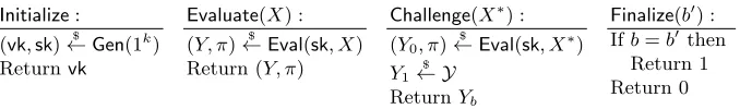
Initialize:
(vk,sk)←$ Gen(1k) Returnvk
Evaluate(X) : (Y, π)←$ Eval(sk, X) Return (Y, π)
Challenge(X∗) : (Y0, π)
$
←Eval(sk, X∗)
Y1 $
← Y
ReturnYb
Finalize(b0) : Ifb=b0 then
Return 1 Return 0
Fig. 1.Procedures defining the VRF security experiment.
Definition 8. (Gen,Eval,Vfy) is a verifiable random function (VRF) if all of the following hold.
Correctness. For all (vk,sk) ←$ Gen(1k) and X ∈ {0,1}∗ holds: if (Y, π) $
←
Eval(sk, X), thenVfy(vk, X, Y, π) = 1. Algorithms Gen,Eval,Vfy are polyno-mial-time.
Unique provability. For all(vk,sk)←$ Gen(1k)and allX ∈ {0,1}∗, there does notexistany tuple(Y0, π0, Y1, π1)such thatY06=Y1andVfy(vk, X, Y0, π0) = Vfy(vk, X, Y1, π1) = 1.
output of the game. Moreover,Amay arbitrarily issueEvaluate-queries, but only after querying Initializeand before querying Finalize. We say thatA is
legitimate, ifAnever queries Evaluate(X)andChallenge(X∗)withX =X∗
throughout the game. We define the advantage ofAin breaking the pseudo-randomness as
AdvVRFA (k) := Pr
GAVRF= 1
−1/2
5
Verifiable Random Functions from cAHFs
In this section, we show a new construction of VRFs. Our construction is closely related to the verifiable random function of Jager [26], which uses a balanced AHF based on error-correcting codes. We show how the error correcting codes can be replaced by a standard hash function by using computational AHFs (cAHFs). We then show how cAHFs are used in a proof in Section 5.3. Further-more, we improve Jager’s VRF with a new proof technique that allows us to halve the size of public verification keys and secret keys.
5.1 Bilinear Groups.
Our VRF construction usesBilinear Groups. We assume that they are generated based on the security parameter. Following [23], we refer to such a generation algorithm as Bilinear Group Generator as defined below.
Definition 9. ABilinear Group Generatoris a probabilistic polynomitime al-gorithmGrpGenthat takes as input a security parameterk(in unary) and outputs
Π = (p,G,GT,◦,◦T, e, φ(1)) $
←GrpGen(1k)such that the following requirements
are satisfied.
1. pis a prime andlog(p)∈Ω(k)
2. GandGT are subsets of{0,1}∗, defined by algorithmic descriptions of maps
φ:Zp→GandφT :Zp→GT.
3. ◦ and ◦T are algorithmic descriptions of efficiently computable (in the
se-curity parameter) maps ◦ : G×G → G and ◦T : GT ×GT → GT, such
that
a) (G,◦)and(GT,◦T)form algebraic groups,
b) φis a group isomorphism from (Zp,+) to(G,◦)and c) φT is a group isomorphism from(Zp,+) to(GT,◦T).
4. e is an algorithmic description of an efficiently computable (in the secu-rity parameter) bilinear map e : G×G → GT. We require that e is
non-degenerate, that is,
x6= 0⇒e(φ(x), φ(x))6=φT(0).
The unique provability property of VRFs requires each group element from the bilinear group to have a unique representation. Therefore, we use the notion of
us to formally proveUnique Provability of our VRF by ensuring that each group element has a unique representation that can efficiently be verified. Formally, we define certified bilinear groups as follows.
Definition 10. We say that group generator GrpGen is certified, if there exist deterministic polynomial-time (in the security parameter) algorithmsGrpVfyand GrpElemVfy with the following properties.
Parameter Validation. Given the security parameter (in unary) and a string
Π, which is not necessarily generated by GrpGen, algorithm GrpVfy(1k, Π)
outputs 1 if and only if Π has the form
Π = (p,G,GT,◦,◦T, e, φ(1))
and all requirements from Definition 9 are satisfied.
Recognition and Unique Representation of Elements of G. Furthermore, we require that each element inGhas a uniquerepresentation, which can be efficiently recognized. That is, on input the security parameter (in unary) and two strings Π and s, GrpElemVfy(1k, Π, s) outputs 1 if and only if
GrpVfy(1k, Π) = 1 and it holds that s = φ(x) for some x ∈
Zp. Here
φ: Zp →G denotes the fixed group isomorphism contained in Π to specify the representation of elements ofG.
Our definition of certifiedness deviates from the original definition [23] in two regards. First, in addition toGrpVfy, we also require the existence of an algorithm
GrpElemVfy that is used to verify the encoding of a group element, whereas in [23],GrpVfyserves both purposes. Second, the security parameter (in unary) is an input to both verification algorithms in our definition.
5.2 VRF Construction
Let H = {H : {0,1}∗ → {0,1}n} be a family of keyed hash functions for some n ∈ N, let GrpGen be a certified bilinear group generator and let VF =
(Gen,Eval,Vfy) be the following algorithms.
Key generation. Gen(1k) runsΠ←$ GrpGen(1k), chooses a random hash func-tion H← H$ and random generators g, h ←$ G, where G is from Π, and
αi $
←Zp fori∈[n+ 1]0. It then defines gi:=gαi and the keys as
vk:= H, Π, g, h,{gi}i∈[n+1]0
and sk:={αi :i∈[n+ 1]0}.
Evaluation. On input vk,sk andX ∈ {0,1}∗,Evalcomputes (H
1, . . . , Hn) :=
H(X),
αX:=α0·
n
Y
i=1
αHi i
!
To compute the proof, it setsπ0:=gα0 and then computesπ1, . . . , πn as
πi:=π
αHii i−1
fori∈[n]. Finally, it setsπn+1:=π
αn+1
n and outputs (Y, π= (π1, . . . , πn+1)).
Verification. Given 1k, vk, X ∈ {0,1}∗ and (Y, π= (π
1, . . . , πn+1)),Vfy tests
ifY andπcontain only valid group elements usingGrpVfyandGrpElemVfy, and outputs 0 if not. Then it computes (H1, . . . , Hn) := H(X) ∈ {0,1}n, definesπ0:=g0, and outputs 1 if and only if for alln∈[n] it holds that
e(πi, g) =
(
e(πi−1, g) ifHi= 0 and
e(πi−1, gi) ifHi= 1,
(8)
and both
e(πn+1, g) =e(πn, gn+1) and Y =e(πn+1, h) (9)
hold.
Comparison to Jager’s VRF. Our construction improves Jager’s VRF in two aspects. First, our verification and secret key containonly one element for each
i ∈[n], compared to two in Jager’s VRF. This improvement is possible by en-coding the keys of the cAHF into the public and secret keys in a more efficient way. We explain this technique in detail in the proof of Theorem 5. The sec-ond improvement is that we instantiate the VRF with a cAHF instead of an bAHF.Therefore, theEvalandVfyapplya standard hash function instead of an error correcting code to each input. This changes the input space of the VRF from {0,1}k to {0,1}∗. In the same way, cAHFs are applicable to the VRFs of Katsumata [29] and Yamada [50]. Notice, that the first improvement is also applicable when the VRF is instantiated with a bAHF instead of a cAHF.
Remark 4. The termsαn+1 andgn+1 in our construction are equivalent to
ap-pending a bit that is always set to one to each output of the hash function. This ensures that there is no input to the hash function resulting in an all-zero output, which is needed in the security proof. Alternatively, we could assume preimage resistance of the hash function and use that there is no efficient adversary that is able to find a preimage for the all-zeros output. We could then guess a position that is one for all inputs provided by the adversary. We chose to introduceαn+1
andgn+1 instead for simplicity and clarity.
Correctness. For any k ∈ N and any X ∈ {0,1}∗, let (vk,sk) ←$ Gen(1k) and
(Y, π) ← Eval(sk, X). We now consider the behaviour of Vfy(1k,vk, X,(Y, π)). Since Y and π are results of Eval, both GrpVfy and GrpElemVfy output 1 and thusVfydoes not reject the input. Now let (H1, . . . , Hn) :=H(X) andπ0:=g0.
Then for alln∈[n], we have
e(πi, g) =e
παHii
i−1
=
( e(πα0i
i−1, g) =e(πi−1, g) ifHi= 0 and
e(πα1i
Therefore, Equation 8 is fulfilled. Furthermore, we have
e(πn+1, g) =e(πnαn+1, g) =e(πn, gn+1),
which fulfills the first part of Equation 9. Moreover, notice that for all i∈[n], we have
πi=gα0 Qi
j=1α Hj
j and πn+1=παn+1
n =g
α0 Qi−1
j=1α Hj j
αn+1
=gαX. Thus, e(πn+1, h) = e(gαX, h) =e(g, h)αX holds, fulfilling Equation 9’s second
part. Hence, Vfy outputs 1 on input (1k,vk, X,(Y, π)). Finally, as can easily be verified,Gen,EvalandVfy are all polynomial-time algorithms.
Unique Provability. We show that for any (vk,sk)←$ Gen(1k) andX ∈ {0,1}∗, there are unique Y, π such that Vfy(1k,vk, X, Y, π) = 1. Let (H
1, . . . , Hn) :=
H(X), then, since elements from G and GT have an unique encoding, πi =
π(αi)Hi
i−1 is the unique group element fulfilling Equation 8. By induction, πi is therefore uniquely defined for alln∈[n]. Analogously,πn+1 is uniquely defined
by the first part of Equation 9. Finally, since πn+1 is uniquely defined, so isY
by the second part of Equation 9.
Pseudorandomness. We will prove the pseudorandomness of our construction based on the q-decisional Diffie-Hellman assumption, also used when proving Pseudorandomness of Jager’s VRF [26], with smallq=dlog(4tA(2tA−1)/A))e=
O(logk).
Definition 11. For a bilinear group generator GrpGen, let GqB-DDH(k) be the following game. The experiment runs Π ←$ GrpGen(1k), samples g, h $
← G,
x ←$ Z|G| and b
$
← {0,1}. Then it defines T0 := e(g, h)x
q+1
and T1
$
← GT.
Finally, it runs b0 ← B$ (g, gx, . . . , gxq, h, Tb), and outputs 1 if b = b0, and 0
otherwise. We denote with
AdvBq-DDH(k) := PrhGBq-DDH(k) = 1i−1/2
the advantageof B in breaking the q-DDH-assumption for groups generated by GrpGen, where the probability is taken over the randomness of the challenger and
B. We say that the q-DDH-assumption holds relative to GrpGen, ifAdvqB-DDH(k)
is negligible in kfor all PPT algorithms B.
Note that the q-DDH assumption is trivially implied by the decisional q+ 1 Bilinear Diffie-Hellman Exponent assumption introduced in [10].
Theorem 5. If VF is instantiated with the family of computational admissible hash functions from Theorem 4, then for any legitimate attacker A that breaks the pseudorandomnessofVF in timetAwith advantageA:=AdvVRFA (k), there exists an algorithm B that, given (sufficiently close approximations of )tA and
A, breaks theq-DDHassumption withq=dlog(4tA(2tA−1)/A)ein timetB≈
tAand with advantage
Remarkably, the proof of Theorem 5 is significantly simpler than the correspond-ing AHF-based proof from [26].
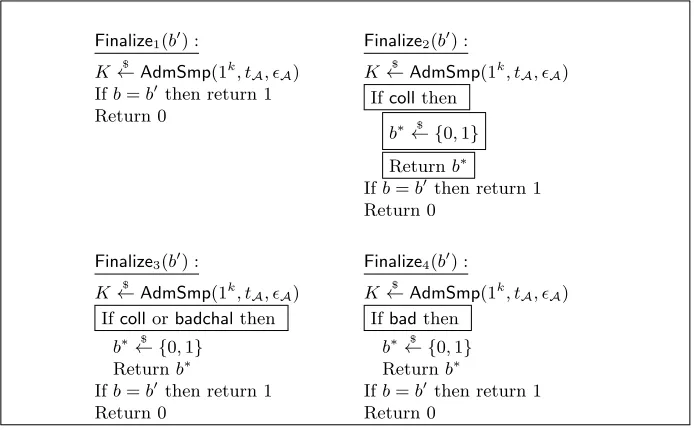
5.3 Proof of Theorem 5
We prove the theorem with a sequence of games. In the sequel let us write Ei to denote the event that Gamei outputs “1”.
Finalize1(b0) :
K←$ AdmSmp(1k, t
A, A)
Ifb=b0 then return 1 Return 0
Finalize2(b0) :
K←$ AdmSmp(1k, t
A, A)
Ifcollthen
b∗← {$ 0,1}
Returnb∗
Ifb=b0 then return 1 Return 0
Finalize3(b0) :
K←$ AdmSmp(1k, tA, A)
Ifcollorbadchalthen
b∗← {$ 0,1}
Returnb∗
Ifb=b0 then return 1 Return 0
Finalize4(b0) :
K←$ AdmSmp(1k, tA, A)
Ifbadthen
b∗← {$ 0,1}
Returnb∗
Ifb=b0 then return 1 Return 0
Fig. 2.Procedures used in the proof of Theorem 5. New or modified statements are highlighted in boxes.
Game 0. This is the original VRF security game, as described in Definition 8. By definition, we have
Pr [E0] = 1/2 +AdvVRFA (k)
as
badchal ⇐⇒ FK,H(X∗)6= 0
coll ⇐⇒ ∃i, j withX(i)6=X(j)s.t.
∀`∈[n] :H(X(i))`=H(X(j))`∨K`=⊥
like in Definition 6. Note that we denote withX(1), . . . , X(Q)the values queried
byAto Evaluate, and with X∗ the value queried to Challenge. These modifica-tions are purely conceptual and perfectly hidden fromA, such that we have
Pr [E1] = Pr [E0].
Game 2. This game proceeds identically to Game 1, except that the challenger aborts if eventcolloccurs. We formally express this change by replacingFinalize1
withFinalize2from Figure 1. By applying Shoup’s Difference Lemma [42], we get
Pr [E2]≥Pr [E1]−Pr [coll].
Game 3. This game proceeds identically to Game 2, except that we replace
Finalize2 withFinalize3, which outputs a random bit ifbadchaloccurs. We have
Pr [E3] = Pr [E3∧badchal] + Pr [E3∧ ¬badchal]
= Pr [E3|badchal] (1−Pr [¬badchal)]) + Pr [E3| ¬badchal] Pr [¬badchal]
= 1/2 + Pr [¬badchal] (Pr [E3| ¬badchal]−1/2)
= 1/2 + Pr [¬badchal] (Pr [E2| ¬badchal]−1/2)
= 1/2 + Pr [¬badchal] (Pr [E2]−1/2)
The third equality uses that Pr [E3|badchal] = 1/2, since a random bit is
re-turned ifbadchaloccurs, the fourth uses that by definition of the games it holds that Pr [E3| ¬badchal] = Pr [E2| ¬badchal], and the last uses Pr [E2| ¬badchal] =
Pr [E2], since Game 2 is independent ofbadchal. This is becauseK is only
sam-pled after A made all its queries and stated its challenge and K is therefore perfectly hidden fromA.
Game 4. We replace events badchaland collwith an equivalent event, in order to simplify the construction of adversary B. We let baddenote the event that
coll∨badchal. In Game 3 the experiment outputs a random bit b∗ ← {$ 0,1}
if (badchal∨coll) occurs. Now we output a random bit if bad occurs, which is equivalent. Formally, we achieve this by replacing Finalize3 with Finalize4 as defined in Figure 1, and get
Summing up probabilities from Game 0 to Game 4, we get
Pr [E4]≥1/2 + Pr [¬badchal] (Pr [E0]−1/2−Pr [coll])
= 1/2 + Pr [¬badchal] (A−Pr [coll])
≥1/2 +τ(k) (10)
for some non-negligible function τ(k), where the last inequality is due to the definition of cAHFs (see Equation 7).
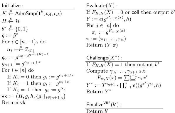
Reduction from the q-DDH assumption. Now we are ready to describe our al-gorithmB that solves the q-DDH problem byperfectly simulating Game 4 for adversaryA. When instantiated with the computational AHF from Theorem 4, a q-DDH instance withq=dlog(4tA(2tA−1)/Aeis sufficient.
The only minor difference between Game 4 and the simulation by B is that B aborts “as early as possible”. That is, it samples the AHF key K ←$
AdmSmp(1k, t
A, A) and random bitb∗ already in the Initializeprocedure, and checks whether badoccurs after each Evaluateor Challenge query ofA. If bad
occurs, then it immediately outputsb∗, rather than waiting for the adversary to queryFinalize. Obviously, this does not modify the probability ofE4. We proceed
by describing B.
Description of algorithmB. The input ofBis theq-DDH-challenge (˜g,g˜x, . . . ,˜gxq
,
h, T). Bfirst tests ˜gx= 1. Since ˜? g is a generator of G, this holds if and only if
x= 0. In this case,B tests e(1, h)=? T and outputs 0 if the statement is true and 1 otherwise. Obviously, this is the correct solution to theq-DDH-challenge ifx= 0. We therefore assumex6= 0 for the remainder of the proof.
Recall thatAis playing the pseudorandomness game for the VRF from Def-inition 8, meaning it tries to distinguish a VRF output from a random value with the help of Initialize,Evaluate,Challengeand Finalize.Bsimulates these op-erations by executing the corresponding procedures from Figure 3. Finally, B
outputs either the random bit b∗ if event bad occurs, or otherwise whatever
Finalize returns. In Figure 3, we denote the number of positions inK that are not 1 byσ(K).
Initialization. The values (˜g, h,˜gx) inInitializeare from theq-DDH-challenge. B computes thegi-values exactly as in the originalGen-algorithm for mosti∈[n] by choosing αi
$
←Z|G|and settinggi:=g
αi, but with the exception that
gi:=
(
gαi+1/x ifK
i= 0
gαi+x ifK
i= 1
for alli∈[n] withKi6=⊥. Note that due to our choice of a cAHF in Theorem 5, we have thatσ(K)≤q. Therefore,Bcan computegα0+xq−σ(K)−1 sinceq−σ(K)− 1 is at least−1 and at mostq−1, andg1/x= ˜g, . . . , gxq−1 = ˜gxq are part of the
q-DDH-challenge.Bcan compute gαi+1/x for the same reason. Allg
Initialize:
K←$ AdmSmp(1k, tA, A)
H ← H$
b∗← {$ 0,1}
g:= ˜gx
Fori∈[n+ 1]0 do
αi=
$
←Z|G|
g0:=gα0+x q−σ(K)−1
gn+1:=gαn+1+x Fori∈[n] do
IfKi= 0 thengi:=gαi+1/x
IfKi= 1 thengi:=gαi+x
IfKi=⊥thengi:=gαi
vk:= H, g, h,{gi}i∈[n+1]0
Return vk
Evaluate(X) :
IfFK,H(X) = 0 orcollthen outputb∗
Y :=e(gPw,X(x), h) Forj∈[n] do
πj:=gPw,X(x)
π:= (π1, . . . , πn)
Return (Y, π)
Challenge(X∗) :
IfFK,H(X) = 1 then outputb∗
Computeγ0, . . . , γq+1s.t.
Pw,X(x) =Pqi=0+1γixi
Y∗:=Tγq+1·Qq i=1e((g
xi)γi, h) ReturnY∗
FinalizeVRF(b0
) : Returnb0
Fig. 3.Procedures for the simulation of the VRF pseudorandomness experiment byB.
Helping definitions. To explain howBresponds toEvaluateandChallengequeries made by A, we define four setsIw,X, Iw,X0 , I
1
w,X andIw,X⊥ , which depend on a VRF inputX ∈ {0,1}∗ and an integer w∈[n]. I
w,X ⊆ [w]⊆[n] is the set of all indices such thatH(X)i= 1. The other sets partitionIw,X in the respective subsets of indices whereKi is 0,1 or⊥. Formally, the sets are defined as follows.
Iw,X :={i∈[w] :H(X)i= 1},
Iw,X0 :={i∈[w] :H(X)i= 1∧Ki= 0},
Iw,X1 :={i∈[w] :H(X)i= 1∧Ki= 1} and
Iw,X⊥ :={i∈[w] :H(X)i= 1∧Ki=⊥},
where K and H are fromB’s choice inInitializein Figure 3. Note that Iw,X =
I0
w,X∪I
1
w,X∪I
⊥
w,X. Based on these sets, we define polynomialsPw,X(x). We let
P0,X(x) :=α0+xq−σ(K)−1 and define
Pw,X(x) =
Pw−1,X(x)·(αi+ 1/x) ifw∈Iw,X0 ,
Pw−1,X(x)·(αi+x) ifw∈Iw,X1 ,
Pw−1,X(x)·αi ifw∈Iw,X⊥ and
Pw−1,X(x) otherwise, forw∈[n] andX ∈ {0,1}∗. Finally, we defineP
n+1,X(x) :=Pn,X(x)·(αn+1+x).
Lemma 2. Let I0
w,X andI
1
w,X be as above, then
Iw,X0 ≤q−σ(K) and
Iw,X1 ≤σ(K)
holds for all w∈[n]. Furthermore, define Pw,X as above, then deg(Pw,X) =q−σ(K)−1−
Iw,X0 +
Iw,X1
holds for allw∈[n], wheredegdenotes the degree of a polynomial. In particular, we have
−1≤deg(Pw,X)≤q−1
for allw∈[n]. Note that we simplify the notation by writingdeg(f) =−k for a rational function f such that1/f is a polynomial of degreek∈N.
We postpone the proof of Lemma 2 to Section 5.4 as to not interrupt the proof of Theorem 5. Similarly to [26], we observe the following.
1. For allXwithFK,H(X) = 1 andw∈[n+1]0, we have−1≤deg(Pw,X(x))≤
q−1. Note that in contrast to Lemma 2, the bound also holds forw=n+ 1. For this, observe that for allX withFK,H(X) = 1, there is ani∈[n] such that Ki 6= ⊥ and Ki 6= H(X)i. Therefore, at least one of the following conditions hold.
Iw,X0
>0 for allw≥i
Iw,X1
< q−σ(K) for all w∈[n]
By Lemma 2, we therefore have deg(Pn,X)≤q−2 implying deg(Pn+1,X)≤
q−1. Hence,Bcan efficiently computegPw,X(x)= ˜gx·Pw,X(x)for allw∈[n+ 1]0. To this end,Bfirst computes the coefficientsγ0, . . . , γqof the polynomial
x·Pw,X(x) =P
q
i=0γixi with degree at mostq, and then ˜
gx·Pw,X(x):= ˜gPqi=0γixi= q
Y
i=0
(˜gxi)γi
using the terms (˜g,g˜x, . . . ,˜gxq) from theq-DDHchallenge.
2. If FK,H(X) = 0, then H(X)i =Ki for all i∈ [n] where Ki 6=⊥and thus
I0
n,X
= 0 and I1
n,X
=σ(K) hold. By Lemma 2,x·Pn+1,X(x) therefore has degreeq+ 1. We do not know how B can efficiently computegPn+1,X(x) = ˜
gx·Pn+1,X(x)in this case.
Responding toEvaluate-queries. As depicted in Figure 3, ifFK,H(X(i)) = 1, then procedureEvaluatecan compute the group elementsgPw,X(x)as explained above. Note that in this case the response to theEvaluate(X(i))-query ofAis correct.
Moreover,Boutputs the random bitb∗ and aborts if there was an earlier query
X(j)to Evaluatesuch that the firstqpositions ofH(X(j)) andH(X(i)) match,
Responding to theChallenge-query. IfFK,H(X∗) = 0, then procedureChallenge computes
Y∗:=Tγq+1·
q
Y
i=0
e((˜gxi)γi, h) =Tγq+1·e(˜gPqi=0γixi, h)
whereγ0, . . . , γq+1are the coefficients of the degree-(q+1)-polynomialx·Pn+1,X∗(x) =
Pq+1
i=0γixi. Note that ifT =e(˜g, h)x q+1
, then it holds thatY∗=Vsk(X∗).
More-over, ifT is uniformly random, then so isY∗. IfFK,H(X∗) = 1, thenBoutputs the random bitb∗ and aborts.
B’s running time. The running timetBofBconsists of the running timetAofA plus the time required to simulate the oracles as depicted in Figure 3. The latter step essentially consists of the operations defined in the construction of the VRF in Section 5.2 plus minor operations like samplingK, evaluatingFK,H, checking for collisions, calculate theγi to computegPw,X(x) and some group operations to compute thegi. Thus, we havetB≈tA.
B’s success probability. Let c ∈ {0,1} denote the random bit chosen by the
q-DDH challenger. B perfectly simulates GAVRF(k) withb =c. Hence, by Equa-tion 10, we get
AdvqB-DDH(k)≥Pr [E4]≥1/2 +τ(k)
for a non-negligible functionτ. In particular, when instantiated concretely with the computational AHF from Theorem 4, then we have
AdvqB-DDH(k)≥1/2 +2A/(32t2A−16tA).
5.4 Proof of Lemma 2
Observe that by the Definition ofAdmSmpin Theorem 4 and the choice ofqin Theorem 5 we have σ(K) ≤q. Furthermore, In,X1 contains up to one element for each i∈[n] such that Ki= 1, which are at most σ(K) many. Analogously,
Iw,X0 can contain at mostq−σ(K) elements sinceKhas onlyq−σ(K) positions where it is 0. We proceed by proving that
deg(Pw,X) =q−σ(K)−1−
IK,w,X0 +
IK,w,X1 (11)
holds for allw∈[n]. Observe that in the definition ofPw,X eachi∈Iw,X0 adds a factor (αi+ 1/x) toPw−1,X and by that decreases the degree of the polynomial by one. Analogously, each element inI1
w,Xincreases the degree of the polynomial by one. Finally,P0,X is defined as (α0+xq−σ(K)−1) yielding, together with the
upper bounds on|Iw,X|
0
and|Iw,X|
1
above, Equation 11. We finish the proof of Lemma 2, by showing that
holds for allw∈[n]. By Equation 11 and |Iw,X| ≤σ(K), the following holds. deg(Pw,X) =q−σ(K)−1−
Iw,X0 +
Iw,X1
≤q−σ(K)−1 +Iw,X1
≤q−σ(K)−1 +σ(K) =q−1.
We conclude the lower bound analogously by applying Equation 11 and|Iw,X| ≤
q−σ(K).
deg(Pw,X) =q−σ(K)−1−
Iw,X0 +
Iw,X1
≥q−σ(K)−1−Iw,X0
≥q−σ(K)−1−q−σ(K) =−1
6
Comparison of VRF Instantiations
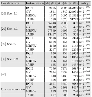
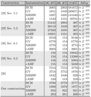
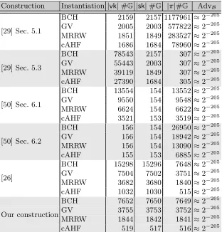
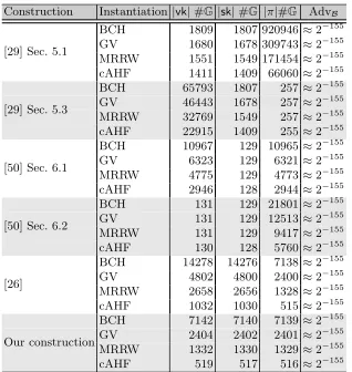
We compare key and proof sizes of the VRFs from Katsumata [29], Yamada [50], Jager [26] and our VRF from Section 5.3 in two different types of instantiation: using bAHFs with ECCs and using cAHFs with TCRHFs from Section 3.1. We do not compare Yamada’s third VRF, because it relies on a much stronger polynomial q-type assumption [50, Appendix C (in the eprint version)]. Com-paring the concrete number of group elements in keys and proofs shows that instantiating the VRFs with cAHFssignificantly reduces the key and proof sizes. Furthermore, comparing our new VRF in Section 5.2 to any of the other VRFs shows that our new VRF haseither significantly smaller secret keys, verification keys or proofs than each other VRF.
Formulas for key and proof sizes. Table 1 shows the sizes of the verification keys
|vk|, secret keys|sk|and proofs|π|as the number of group elements they contain in dependence ofk, Q, , δandt. The caption precisely explains how the key and proof sizes relate to these variables. Furthermore, the table shows the advantage of the solver AdvBagainst the respective hard problem. For the VRFs of of [29] and [50], this is the q-DBDHI assumption introduced by Boneh and Boyen [8]. For our VRF and Jager’s VRF [26] this is theq-DDHassumption. Even though the assumptions differ, the key and proof sizes are comparable for the following reasons.
1. Cheons algorithm [16] is the most efficient known generic algorithm to solve both, theq-DDHassumption and theq-DBDHIassumption.
Construction Instantiation |vk|#G |sk|#G |π|#G AdvB
ECCs 3 +ζd dζ+ 1 d+dn+ζ+ 1 τ+stat
[29] Sec. 5.1
cAHF 3 +ζtcrhj ζtcrh+ 1j+j(ntcrh) +ζtcrh+ 1τtcrh+stat
ECCs 3 +d(2ζ/2+2−2) dζ+ 1 2d−1 τ+stat
[29] Sec. 5.3
cAHF 3 +j(2ζtcrh/2+2−2)jζtcrh+ 1 2j−1τtcrh+stat
ECCs dn1+ 2 d dn2 τ+stat
[50] Sec. 6.1
cAHF jntcrh
1 + 2 j jntcrh2 τtcrh+stat
ECCs d+ 2 d d(n1+n2−1) τ+stat
[50] Sec. 6.3
cAHF j+ 2 j j(ntcrh
1 +ntcrh2 −1)τtcrh+stat
ECCs 2n+ 2 2n n τ
[26]
cAHFs 2ntcrh+ 2 2ntcrh ntcrh τtcrh
ECCs n+ 4 n+ 2 n+ 1 τ
Our construction
cAHFs (as shown) ntcrh+ 4 ntcrh+ 2 ntcrh+ 1 τtcrh
Table 1.The sizes of vk,sk,π as the number of group elements and the advantage of the solver in the security proof for the instantiation of our VRF and the VRFS of Jager [26], Yamada [50] and Katsumata [29]. d =b(2Q+Q/)/log(1−δ)c is the number of positions in the key of the bAHF that are not⊥. Note that [29,26,50] all chose d in this way. For the VRFs from Katsumata [29], ζ = blog(2n)c+ 1 is the number of bits required to encode an element from [2n].τ is as in Definition 3 and de-scribes the advantage of a solver against the underlyingq-type assumption withq:=d
for the instantiation using ECCs and q :=j using TCRHFs.stat represents statisti-cally negligible values introduced in the security proofs of Yamada’s and Katsumata’s VRFs [50,29]. Note that for Yamada’s VRFs [50], n1, n2 ∈ N can be chosen freely
such that n = n1n2. Analogously, we have ntcrh := 2k+ 3 as the output length of the truncation collision resistant hash function,ζtcrhis the number of bits required to encode an element from [ntcrh]. As in Theorem 4 the length of the prefix used for the TCRHFs is j:=d4t(2t−1)/e. Again,ntcrh1 , ntcrh2 ∈Ncan be chosen freely such that
ntcrh=ntcrh
1 ntcrh2 . Finally, we haveτtcrh=2/(32t2−16t) from Theorem 4.
Instantiation choices. The concrete number of group elements in keys and proofs depends on some instantiation choices, which we describe here. Since the VRF instantiation with cAHFs takes inputs from {0,1}∗, we level the playing field by assuming that the instantiations using ECCs first hash the inputs with a collision resistant hash function H :{0,1}∗ → {0,1}α and thus the VRFs also take inputs from{0,1}∗. We letα= 2k, wherek is the security parameter, to ensure the collision resistance of H against birthday attacks. Hence, when an ECC C is used in an instantiation, then C takes inputs from {0,1}2k. We list the key sizes of the different VRFs, instantiated with cAHFs and with ECCs in Table 2.
– We consider primitive BCH codes that we puncture to achieve the desired relative minimal distance. Again, tables in for example [41, Table 9.1] only list codes for lengths up to 1023. We therefore wrote a small program that finds the most suited primitive BCH code for this purpose. It can be found at
https://github.com/DavidNiehues/bch-code-search. The program con-siders the Bose distance of the BCH codes instead of the design distance. The caption of Table 2 states the used primitive BCH code explicitly. – Furthermore, we present key and proof sizes under the assumptions that
ECCs on the GV and MRRW bound can be efficiently instantiated.
Assuming instantiations with ECCs on the GV and MRRW bound gives the instantiation with bAHFs and ECCs an advantage over instantiations using cAHFs with TCRHFs, since ECCs on the MRRW-bound are the best theo-retically possible ECCs and it is not known whether ECCs on the GV-bound can be constructed efficiently.
In the calculation of the key sizes of Yamada’s VRFs [50], we pickn1 =n2
asd√nein order to make the parameter sizes comparable. We make this choice, because Yamada suggest pickingn1andn2close to
√
n[50] and because choosing actual divisors of n would make key and proof sizes heavily depend on the factorization ofn. This would lead to misleading results. Furthermore, we chose
δ such that all instantiations achieve the same advantage of the solver. This makes the different instantiations comparable. Note that we did not incorporate the statistically negligible termsstatin the calculation of the advantage.
Smaller keys and proofs using cAHFs. Table 2 shows the concrete number of group elements of the different instantiations in the setting withk= 128, Q= 225,t= 250 and= 2−25. The instantiation of the VRFs with cAHFs improves the size of keys and proofs significantly, even compared to bAHFs instantiated with the best theoretically possible ECCs on the MRRW bound. Concretely, using cAHFs with TCRHFs instead of bAHFs with ECCs on the MRRW boundreduces the size of the proofs of the VRF in Section 5.1 in [29] by≈61% in the setting of Table 2. Compared to an instantiation with ECCs on the GV bound, we reduce the proof size by even ≈ 78%. Compared to the instanitation with punctured primitive BCH codes, the improvement is even ≈ 87%. Particularly, keys and proofs whose size depends linearly onnshrink when the VRFs are instantiated with cAHFs. Over all key and proof sizes affected by the improvement, the reduction amounts for at least 9% of the size of an instantiation with ECCs on the MRRW bound. Note that the size of all keys and proofs stays at least the same. Hence, by making an additional (but from a practical point of view plausible and natural) hardness assumption, we can reduce the key and proof sizes significantly, which may be useful for many practical applications of VRF. Furthermore, it hints at the usefulness of cAHFs for other primitives.
![Table 1. The sizes ofof the solver in the security proof for the instantiation of our VRF and the VRFSof Jager [26], Yamada [50] and Katsumata [29]](https://thumb-us.123doks.com/thumbv2/123dok_us/7991427.1326455/27.612.138.481.114.244/table-solver-security-instantiation-vrfsof-jager-yamada-katsumata.webp)