A Self-Adaptive Discrete PSO Algorithm with
Heterogeneous Parameter Values for Dynamic TSP
Łukasz Str ˛ak , Rafał Skinderowicz , Urszula Boryczka and Arkadiusz Nowakowski University of Silesia in Katowice, Institute of Computer Science, B˛edzi ´nska 39, 41-205 Sosnowiec, Poland
* Correspondence: [email protected]
This paper presents a discrete particle swarm optimization (DPSO) algorithm with heterogeneous 1
(non-uniform) parameter values for solving the dynamic travelling salesman problem (DTSP). The 2
DTSP can be modelled as a sequence of static sub-problems, each of which is an instance of the TSP. 3
We present a method for automatically setting the values of the DPSO parameters without three 4
parameters, which can be defined based on the size of the problem, the size of the particle swarm, the 5
number of iterations, and the particle neighbourhood size. We show that the diversity of parameter 6
values has a positive effect on the quality of the generated results. We compare the performance of the 7
proposed heterogeneous DPSO with two ant colony optimization (ACO) algorithms. The proposed 8
algorithm outperforms the base DPSO and is competitive with the ACO. 9
1. Introduction 10
In recent years, considerable attention has been paid to optimization in a dynamically changing 11
environment in which the problem being solved is modified periodically or even continuously [1]. 12
This interest is related to the growing practical demand for such solutions. For example, in the problem 13
of task scheduling in a factory, a change to the production schedule might be required if there is a 14
malfunction of part of the production line. The optimization algorithms should be able to adapt 15
rapidly to changes so that the quality of the generated solutions remains acceptable. A problem in 16
which the input data are conditional upon time is called a dynamic optimization problem (DOP). 17
The aim of optimization in a DOP is a constant trace and an adaptation to changes, in order to allow 18
high-quality solutions to be found efficiently [2]. 19
20
A simple example of a DOP is the dynamic travelling salesman problem (DTSP). This consists 21
of a sequence of static travelling salesman problem (TSP) instances (sub-problems). Each successive 22
sub-problem is created on the basis of the previous one. A portion of the sub-problem’s data is 23
transferred unchanged from the predecessor, while the remaining portion is modified. Figure 1 24
summarizes this concept. 25
Solve sub-problemI0
Static TSP
Solve sub-problemI1
Static TSP
Solve sub-problemI2
Static TSP
Solve sub-problemI3
Static TSP
Change Change Change
Figure 1.An example of a DOP—the DTSP. A change in the problem instance may affect both the distances between the cities and the number of cities (vertices). This figure presents an example of a DTSP that includes a primary sub-problem (I2) and three successive sub-problems.
The aim is to find an optimal solution to every sub-problem. If all the sub-problems are solved to 26
optimality, then the resulting sum of the solution (route) lengths is also minimal. Our DTSP benchmark 27
generator includes the optimal value for every sub-problem; hence, the aim can be expressed in terms 28
of finding the minimal sum of the differences between the generated solutions and the optima for the 29
sub-problems. If the value of the sum is zero, then the optimum value is found for every sub-problem. 30
The particle swarm optimization (PSO) algorithm is an optimization technique created by 31
Kennedy and Eberhart [3] in 1995. This technique is inspired by the natural behaviour of a group of 32
animals, e.g. a shoal of fish or a flock of birds. Every particle represents one of the possible solutions 33
to a problem. In the continuous optimization case, the solution is a point in a real-valued space. The 34
movement of the swarm can be interpreted as searching in the solution space. At the beginning of 35
execution of the algorithm, the position of each particle is chosen randomly. Then, in each iteration of 36
the algorithm, the velocities of the particles are calculated (direction of searching) and their positions 37
are updated. This results in a new solution to the problem. The velocity of the particle is influenced by 38
the best-so-far solution (position) of the swarm and the best-so-far (previous) position of the particle. 39
This process allows the swarm of particles tolearnand move towards the areas of the problem solution 40
space that contain higher-quality solutions. The movement of the swarm in the solution space is 41
described by the following equations: 42
~vk+i 1←ω·~vki
+~U(0,φ1)⊗(
−−−→ pBesti−~xki)
+~U(0,φ2)⊗(
−−−→
gBest−~xik), (1)
~xk+i 1←~xik+~vk+i 1, (2)
~v,~x, −−−→gBest, −−−→pBesti ∈Rn,
whereiindexes the particles,kis the current iteration,~vki is the velocity of theith particle in thekth 43
iteration,~x is the position of the particle equal to one of the solutions of the problem, the function 44
U(0,φ)takes a uniform random value in the range[0,φ], andωis aninertiaparameter. The variables
45
−−−→ pBestiand
−−−→
gBestdenote the best-so-far solutions found by the particle and by the swarm, respectively, 46
andφ1andφ2are cognitive and social parameters, respectively, that scale the influence of −−−→ pBestiand
47 −−−→
gBeston the position of the next particle. 48
Initially, the algorithm was created for optimization in a continuous space, but was later adapted 49
to discrete optimization. In 1997, Kennedy and Eberhart [4] presented the first discrete PSO (DPSO) 50
algorithm, in which the particle position was a binary vector and the velocity (direction of movement 51
through the solution space) was the probability of a binary negation of the bits of the particle position. 52
In 2004, Clerc [5] proposed a new DPSO algorithm and applied it to solve the TSP. In this algorithm, 53
the particle position was a vector of vertices, while the velocity comprised a list of pairs of vertices, 54
which changed in the next solution. In 2007, Shi et al. [6] presented an improved DPSO algorithm, 55
which they used to solve the following TSP instances:eil51,berlin52,st70,eil76, andpr70. In their 56
algorithm, the particle position is a permutation, and its modification resembles the well-known 57
crossover found in genetic algorithms. Shi et al. showed that the proposed algorithm is capable of 58
solving the generalized TSP, in which the edge lengths do not satisfy the triangle inequality. The 59
homogeneous and heterogeneous versions of the DPSO algorithm described in the present paper 60
are based on work by Zhong et al. [7] and on our previous DTSP variant [8]. In the implementation 61
presented here, the particle position comprises a set of edges connecting TSP cities (nodes) and the 62
corresponding probabilities of selecting the edges to the next solution (the next position of the particle). 63
As far as we know, our previous work on applying the DPSO to solving the DTSP was the first 64
publication on this topic in the literature. 65
The original PSO algorithm and its discrete versions are homogeneous, i.e. all particles have 66
the same values of the parameters and hence share the same pattern of moving through a solution 67
space [4]. However, heterogeneous populations are common in the natural environment [9]. One of 68
the most important problems with the PSO concerns the balance between exploration and exploitation. 69
A heterogeneous population allows particles to have various patterns of moving through the solution 70
space and thus to exhibit different levels of emphasis on the exploitation and exploration of the solution 71
the algorithm runtime, and others in the later stages. In this way, the balance between exploration and 73
exploitation can be influenced [10,11]. 74
1.1. Contributions 75
Our previous work has focused mainly on DPSO withhomogeneous(uniform) parameter values [8]. 76
In this paper, we extend our initial work on DPSO in which individual particles may have non-uniform 77
(varying) values of the parameters [12]. Specifically, our contributions are as follows: 78
• We propose a method for automatically setting the values of four crucial DPSO parameters. 79
This method is based on discrete probability distributions defined to diversify the behaviours 80
of the particles in the heterogeneous DPSO. The aim of this diversification is to improve the 81
convergence of the algorithm. 82
• We perform an analysis of the convergence of the proposed algorithm based on computational 83
experiments conducted on a set of DTSP instances of varying sizes. We discuss the relationships 84
between the values of the DPSO parameters and their effect on particle movement through the 85
problem’s solution search space. 86
• We compare the efficiency of the proposed heterogeneous DPSO with that of the base DPSO and 87
two algorithms based on ant colony optimization (ACO). The results show that the proposed 88
algorithm outperforms the base DPSO and is competitive with the ACO-based algorithms. 89
The structure of this paper is as follows. Section 2 presents a review of the literature concerning the 90
DTSP. Section 3 describes the heterogeneous version of PSO. Section 4 gives a brief description of DPSO 91
with pheromone. Section 5 describes the heterogeneous swarm. Section 6 presents our experimental 92
results. Finally, Section 7 presents a summary and conclusions. 93
2. Dynamic Travelling Salesman Problem 94
The dynamic nature of the DTSP can entail changes in the distances between cities (nodes) and in 95
the number of cities to be visited [13,14]. Every data transformation can trigger changes in local and 96
global optima. The distance matrix can be defined as 97
D(t) ={dij(t)}n(t)×n(t), (3)
wheretis time,iandjdenote vertices, andnis the number of vertices. Most often, it is assumed that 98
the time is discrete, and hence the DTSP can be viewed as a series ofstaticTSP instances (Figure1). 99
Each sub-problem can be more or less similar to the previous one, depending on the number of changes 100
and their magnitude. In this paper, we assume that only the distances between the cities are subject to 101
change, while the number of nodes (vertices) remains constant. 102
Obviously, each of the DTSP sub-problems can be solved separately using one of the methods 103
developed for the TSP [15]. Nevertheless, if the differences between consecutive DTSP sub-problems 104
are small, it is possible that the optimal solutions differ only slightly. In such a case, it is possible to use 105
the knowledge gathered while solving the previous sub-problem to speed up solving the current one. 106
A summary of recent research on solving the DTSP that has been presented in the literature is given in 107
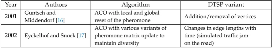
Table1. 108
Table 1. Summary of recent papers on solving the DTSP with computational intelligence methods.
Year Authors Algorithm DTSP variant
2001 Guntsch and Middendorf [16]
ACO with local and global
reset of the pheromone Addition/removal of vertices
2002 Eyckelhof and Snoek [17]
ACO with various variants of pheromone matrix update to maintain diversity
Table 1. Summary of recent papers on solving the DTSP with computational intelligence methods.
Year Authors Algorithm DTSP variant
2006 Li et al. [14] GSInver-Over and Gene Pool withα-measure [18]
CHN145+1: 145 cities and one satellite
2010 Mavrovouniotis and Yang [19]
ACO with immigrants scheme to increase population diversity
Coefficients: frequency and size of changes
2011 Simões and Costa [20] CHC algorithm
A test involving addition of changes and their
subsequent withdrawal [21]. In that way, the optima at the beginning and the end are the same
2014 Tinós et al. [22] EA algorithm Random changes in the problem
2014 Zhang and Zhao [23] Hopfield neural network Simulation of various types of real random events in the street
2016 Eaton et al.[24] ACO with immigrants scheme Changes in edge lengths. Simulated delays of trains
2016 Mavrovouniotis and
Yang [25] MMAS
Encoding of the problem is changed, but the optimal solution remains the same
2017 Mavrovouniotis et al. [26] ACO
Distances between cities are changed. The problem can be transformed to an asymmetric one
3. Heterogeneity 109
Heterogeneity can be defined as the absence of uniformity (diversity). In computational 110
intelligence algorithms, it can appear in many ways. A taxonomy of the various levels of heterogeneity 111
that are possible in the PSO algorithm was given by Montes de Oca et al. [11], who divided 112
heterogeneity into the following four categories: 113
1. Neighbourhood heterogeneity: this concerns cases in which the size of the neighbourhood is different 114
for every particle, and hence the virtual topology of connections between particles is not regular. 115
Some particles can have a wider influence than others on the movement of the swarm. 116
2. Best-particle heterogeneity: here there can be variations in the method of selecting the best 117
particle, i.e. the particle whose position is used when updating the current velocity and position. 118
For instance, one particle might update its position following the best particle in its (small) 119
neighbourhood, while the second particle might be fully informed and follow the global best 120
particle. 121
3. Heterogeneity of the position update strategy: here the particles differ in their patterns of movement 122
(searching) through the solution space. For example, one group of particles mightexplorethe 123
solution space, while the other group might conduct a local search by restricting their velocities 124
or even positions to a certain range. This type of heterogeneity diversifies the population to the 125
greatest extent, since it provides the greatest flexibility in diversifying particle movement. 126
4. Heterogeneity of parameter values: here each particle or group of particles in the swarm can have 127
different values of the parameters. For example, some particles might have a large inertiaωand
128
explore the solution space, whereas other particles might have a small value ofωand perform
129
the search locally (around the best position found). Although this type of heterogeneity is not as 130
flexible as heterogeneity of the position update strategy, it requires relatively few changes to the 131
PSO, since only the values of the particle parameters need be set individually. It is this strategy 132
Although there is a lack of information in the literature with regard to heterogeneity in the case of 134
the DPSO algorithm, it is possible to adapt the solutions proposed for standard PSO. 135
4. DPSO with Pheromone 136
A (homogeneous) DPSO algorithm with pheromone was proposed in our previous work [8], 137
and this section contains only a brief description. Adaptation to a discrete space forces some changes 138
to the original PSO algorithm designed for solving continuous optimization problems. All variables 139
(i.e.XandV) becomesetsof edges instead of real-valued vectors. An edge is represented by a tuple: 140
hp,{a,b}i, whereaandbare endpoints andpis the probability of selecting the edge(a,b)to become 141
part of the constructed solution. The equations governing the movement of the particles become 142
Vik+1=c2·U(0, 1)·(gBest\Xik)
∪c1·U(0, 1)·(pBesti\Xik)
∪ω·Vik, (4)
Xik+1=∆τk(Vik+1)⊕c3·U(0, 1)·Xik, (5)
whereiis the particle index,kis the iteration, andU(0, 1)is a uniform random number from the range 143
[0, 1]. The operators∪and\denote the classical operations on sets, while the multiplication of a set 144
by a scalar (i.e.c2·U(0, 1)·(gBest\Xik)) represents multiplication of thepvalue of each edge by the 145
scalar. The⊕operator does not exist in classical PSO—its purpose in DPSO is to complete the solution 146
with missing edges so that it forms a Hamiltonian cycle. The∆τfunction changes the probabilitypof
147
the edge using the pheromone matrix familiar from ACO. The pheromone has two main functions in 148
the algorithm: 149
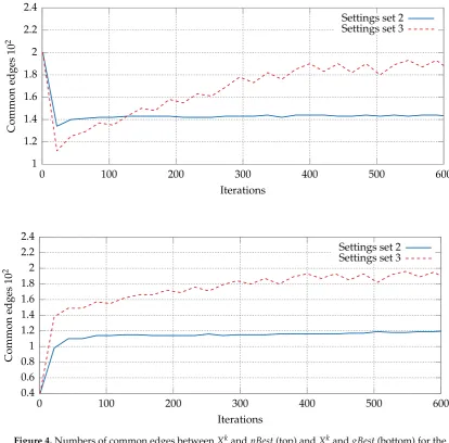
1. It alters the probability of edge selection during the solution construction process; i.e. the higher 150
the value of the pheromone, the greater is the probability of selecting the corresponding edge. 151
In other words, the pheromone serves as an additional memory of the swarm, allowing it to 152
learn the structure of high-quality solutions and, potentially, improve the convergence of the 153
algorithm. 154
2. The pheromone matrix created while solving the current DTSP sub-problem is retained and used 155
when solving the next sub-problem. This allows knowledge about the previous solution search 156
space to be transferred with the aim of helping the construction of high-quality solutions to the 157
current sub-problem. This implicitly assumes that the changes between consecutive sub-problems 158
are not very great, so that the high-quality solutions to the current sub-problem share most of 159
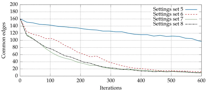
their structure with the high-quality solutions to the previous one. 160
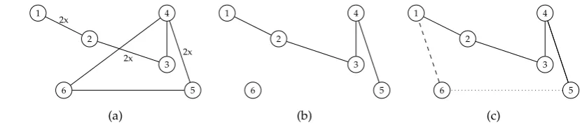
For example, letGube the undirected graph defined as follows:
161
Vu ={1, 2, 3, 4, 5, 6}, |Eu|=
n 2
(all two-pairs combinations of the setGu). Let the first particle in the first iteration represent the solution
162
X10={h1,{1, 4}i,h1,{4, 2}i,h1,{2, 5}i,h1,{5, 3}i,h1,{3, 6}i,h1,{6, 1}i}, V01={h1,{2, 5}i},
gBest={h1,{1, 2}i,h1,{2, 3}i,h1,{3, 4}i,h1,{4, 5}i,h1,{5, 6}i,h1,{6, 1}i}, pBest0={h1,{1, 2}i,h1,{2, 3}i,h1,{3, 5}i,h1,{5, 4}i,h1,{4, 6}i,h1,{6, 1}i}. The result of applying Eq. (4) is
gBest\X10={h1,{1, 2}i,h1,{2, 3}i,h1,{3, 4}i,h1,{4, 5}i,h1,{5, 6}i}, pBest0\X10={h1,{1, 2}i,h1,{2, 3}i,h1,{5, 4}i,h1,{4, 6}i}.
The next velocity of the particleV02after the operation of multiplication byc1·rand(),c2·rand(), or 164
ω·rand()is
165
(gBest\X01)∪(pBesti\X01)∪V01={h0.3,{1, 2}i,h0.1,{2, 3}i,h0.5,{3, 4}i,h0.6,{4, 5}i,h0.1,{5, 6}i, h0.2,{1, 2}i,h0.9,{2, 3}i,h0.7,{5, 4}i,h0.4,{4, 6}i}.
The edge from the previous velocity is not added to the sum, because of the rule forbidding any vertex 166
(node) to occur more than four times (deg(2) =5) [7]. Let us assume that pheromone reinforcement is 167
equal to zero (no influence) and that the random function returns the values 0.1, 0.7, 0.49, 0.5, 0.9, 0.3, 168
0.6, 0.55, 0.39. Then, after the filtration stage, the (incomplete) particle position set is 169
X20={h0.3,{1, 2}i,h0.5,{3, 4}i,h0.6,{4, 5}i,h0.9,{2, 3}i,h0.7,{5, 4}i,h0.4,{4, 6}i}.
The next stage is more restrictive. Any edge that creates an incorrect tour is removed from the set. The 170
edgeh0.4,{4, 6}iis rejected, because deg(4) =3. The edgeh0.7,{5, 4}iis also rejected, because the 171
edge with{4, 5}endpoints already exists in the next position. The next incomplete particle position is 172
X02={h0.3,{1, 2}i,h0.5,{3, 4}i,h0.6,{4, 5}i,h0.9,{2, 3}i}.
At this stage, the first part of Eq. (5) is completed. The operation⊕adds to the result the edge(X2 0) 173
h1,{6, 1}ichosen from the previous particle position set. To complete the set to form the Hamiltonian 174
cycle, the nearest-neighbour heuristic is used and the edgeh1,{5, 6}iis selected. The final particle 175
position is 176
X02={h1,{1, 2}i,h1,{2, 3}i,h1,{3, 4}i,h1,{4, 5}i,h1,{5, 6}i,h1,{6, 1}i}.
Figure2presents a visualization of all the primary operations, i.e. the edges from the particle’s previous 177
positionXik−1before the filtration (a), after the filtration (b), and the final particle position (c). The 178
dashed line marks the edge from Eq. (5) and the dotted line the edge from the completion process (c).
1
2
3 4
5 6
2x
2x 2x
1
2
3 4
5 6
(a)
1
2
3 4
5 6
1
2
3 4
5 6
(b)
1
2
3 4
5 6
1
2
3 4
5 6
(c)
Figure 2.Example of calculation of a new particle position in the DPSO. 179
5. Heterogeneous Swarm 180
The DPSO has four main parameters that influence particle movement through the solution 181
search space:c1,c2,c3, andω. To better understand how the parameter values are set in the proposed
182
heterogeneousDPSO, it is helpful to focus on how the parameters govern the swarm behaviour. Zhong 183
ω ∈ [0, 0.6]. Setting the parameters to small values, i.e. close to the start of the range, forces the
185
particles to change their positions (edges) frequently, since the probability of selecting the edges from 186
the current best positions (local and global) is relatively small. Also, in the initial stage of execution 187
of the algorithm, the pheromone values cannot guide the construction process, since they are also 188
small. On the other hand, setting the parameters to higher values forces the solution construction 189
process to become more exploitative, since the constructed solutions resemble the previously obtained 190
high-quality solutions. Based on our earlier studies of the DPSO algorithm, we have selected the 191
characteristic setsof the parameter values, which are shown in Table2. For each set, we provide a 192
brief description of the corresponding DPSO particle behaviour. Below, we present a more detailed 193
description of the sets, supported by some experimental data analysis. 194
Table 2. Characteristic sets of particle parameter values for the DPSO algorithm along with their influence on particle movement.
No c1 c2 c3 ω Description
1 0.1 0.1 0.1 0.1 Favours quick changes of position 2 2.0 0.1 0.1 0.1 Emphasis on the information frompBest 3 0.1 2.0 0.1 0.1 Emphasis on the information fromgBest 4 0.1 0.1 2.0 0.5 Very slow changes of position
5 0.75 1.0 1.0 0.25 WeakpBest,gBestinfluence 6 1.25 1.5 1.5 0.5 StrongerpBest,gBestinfluence 7 1.5 2.0 2.0 0.5 StrongpBest,gBestinfluence 8 1.75 2.0 2.0 0.75 Very strongpBest,gBestinfluence
Figure3presents the numbers of new edges forXk−1andXk(the previous and current positions). 195
The blue line indicates the particle parameter values, which often change edges (setting 1), and the red 196
line is for more stable particles, with less frequent changes (setting 4). 197
0 2 4 6 8 10 12
0 200 400 600 800 1000 1200 1400 1600 1800
Dif
f.
edges
10
4
Iterations
Settings set 1 Settings set 4
Figure 3.Numbers of new (different) edges betweenXk−1andXk(the previous and current positions) in the DPSO solving the statickroA200TSP instance. The blue line indicates the particles with the first set of values from Table2(setting 1) and the red line is for the more “stable” particles for which the fourth set (setting 4) of parameter values were used. The remaining parameters were taken from Table5. The values were averaged over 30 runs of the algorithm.
The first and fourth sets of parameter values from Table2differ in terms of the dynamics of 198
changes in the number of common edges between the current and previous positions of the particle. 199
For the small parameter values taken from the first set, the probability of edge selection to the next 200
position (p) is very small and can only be increased if the corresponding pheromone has a high value. 201
result, the edges from the previous position will be added to the next position of the particle with 203
high probability. Both characteristics can be clearly seen in Figure3. The blue line is below the red one, 204
which means that the position of the particle from the first set has more changed edges. 205
1 1.2 1.4 1.6 1.8 2 2.2 2.4
0 100 200 300 400 500 600
Common
edges
10
2
Iterations
Settings set 2 Settings set 3
0.4 0.6 0.8 1 1.2 1.4 1.6 1.8 2 2.2 2.4
0 100 200 300 400 500 600
Common
edges
10
2
Iterations
Settings set 2 Settings set 3
Figure 4.Numbers of common edges betweenXkandpBest(top) andXkandgBest(bottom) for the second and third sets of characteristic parameter values (Table2). (The DPSO algorithm was run for the statickroA200TSP instance.) The remaining parameters were taken from Table5. The values were averaged over 30 runs of the algorithm.
An analogous comparison can be made for the second and third sets of values shown in Table2. 206
Figure4shows the average numbers of common edges between the current position of a particle,Xk, 207
and the best positions, i.e. the particle’s local bestpBestand the swarm bestgBest. For the second set 208
of parameter values, the number of edges shared withpBestwas higher than for the third set. This 209
was caused by the highc1value, equal to 2, which affected in particular the initial iterations of the 210
algorithm. After the first 100 iterations, the number begins to change aspBestandgBestbecome more 211
similar. This is an effect of the high value of thec2parameter in the third set of parameter values. The 212
bottom plot in Figure4shows the average number of common edges for the setsXkandgBest. We can 213
see a growing similarity of the current positionXkto the current best positionpBest. This effect can be
214
observed for both sets of parameter values. The number of common edges is higher for the third set, 215
0 20 40 60 80 100 120 140 160 180 200
0 100 200 300 400 500 600
Common
edges
Iterations
Settings set 5 Settings set 6 Settings set 7 Settings set 8
Figure 5.Total numbers of common edges between the current position of the particle,Xk, andpBest, and betweenXkandgBestfor the DPSO solving thekroA200TSP instance with the parameters given
by sets 5–8 in Table2. The remaining parameters were taken from Table5. The values were averaged over 30 runs of the algorithm.
An analogous comparison, this time for sets 5–8 from Table2, is presented in Figure5. The largest 217
differences can be observed for the fifth and the sixth sets, and the smallest for the seventh and eighth. 218
This is due mainly to the small differences between the parameter values, namely∆c1 = 0.25 and 219
∆ω=0.25 (the remaining parametersc2andc3have the same value). 220
Based on the number of times each value of a parameter appears in Table2, a discrete probability 221
distribution for the parameters can be defined: 222
1. c1:P(0.1)= 0.4,P(0.75)=0.15,P(1.5)=0.3,P(1.75)=0.15; 223
2. c2andc3:P(0.1)=0.4,P(1)=0.15,P(1.5)=0.15,P(2)=0.3; 224
3. ω:P(0.1)=0.4,P(0.25)=0.2,P(0.5)=0.4.
225
This allows the values of the DPSO parameters to be controlled, while also allowing them to be mixed 226
together; i.e. any combination of the listed values is possible. As a result, we can expect that both 227
the exploration- and exploitation-oriented behaviours of the particles will be present in a swarm, 228
hence increasing the chances of finding high-quality solutions regardless of the “landscape” of the 229
solution space. This also has the advantage of being more computationally efficient compared with a 230
completely random setting (e.g. with uniform probability), since, in the latter case, one would need a 231
larger number of particles to observe a similar mix of characteristic particle behaviours. 232
6. Experimental Results 233
This section is divided into two parts. In the first, we focus on the effect of the parameter values 234
on the performance of individual particles in the heterogeneous DPSO algorithm. In the second, we 235
conduct a comparison between the homogeneous DPSO, the proposed heterogeneous DPSO, and 236
two well-known ACO algorithms, namely the ant colony system (ACS) and population-based ACO 237
(PACO). 238
6.1. Convergence Analysis for Various Sets of Parameters 239
To assess the performance of individual particles in a swarm of the heterogeneous DPSO, we 240
counted the number of times the particle improved the current global best solution gBest. The 241
parameter values were set randomly according to the discrete probability distribution described 242
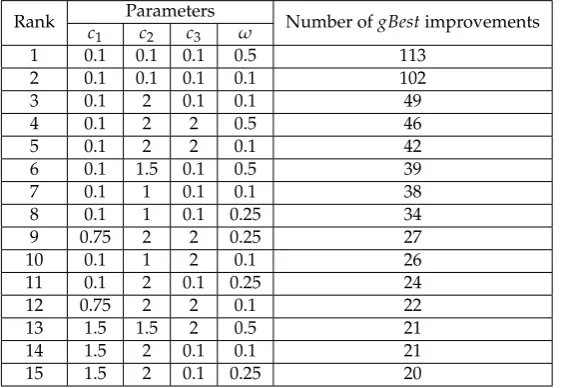
Table3shows the sets of parameter values for which the particles were able to improve the global 244
best solution most frequently. As can be seen, the top two are the sets in which the parametersc1,c2, 245
c3, andωare relatively small. These values favour exploratory behaviour of the DPSO particles, and
246
hence the particles are more likely to find an improved solution, especially in the initial phases of 247
algorithm execution. The set for which the behaviour should be more stable and less exploratory, i.e. 248
withc2=2, turned up as third in the ranking. The relatively large difference of 53 between the second 249
and third positions is also noteworthy. The lower rankings of the particles exhibiting more exploitative 250
behaviour confirm that they could be more important in the later stages of algorithm execution, in 251
which smaller changes to the solution structure are preferred. 252
Table 3.Ranking of parameter values for which the particles in the heterogeneous DPSO were able to improve the global best solution the greatest number of times. The results are accumulated over 30 executions for thegr666TSP instance.
Rank Parameters Number ofgBestimprovements c1 c2 c3 ω
1 0.1 0.1 0.1 0.5 113
2 0.1 0.1 0.1 0.1 102
3 0.1 2 0.1 0.1 49
4 0.1 2 2 0.5 46
5 0.1 2 2 0.1 42
6 0.1 1.5 0.1 0.5 39
7 0.1 1 0.1 0.1 38
8 0.1 1 0.1 0.25 34
9 0.75 2 2 0.25 27
10 0.1 1 2 0.1 26
11 0.1 2 0.1 0.25 24
12 0.75 2 2 0.1 22
13 1.5 1.5 2 0.5 21
14 1.5 2 0.1 0.1 21
15 1.5 2 0.1 0.25 20
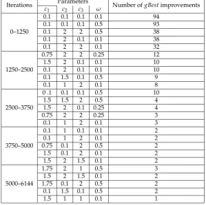
To clarify this distinction, we have analysed which values of the parameters proved to be working 253
best during subsequent phases of algorithm execution. The phases were defined by dividing the total 254
number of iterations into equal parts (intervals). For each interval, we ranked the sets of parameter 255
values based on the number of times they led to a new global best solution within the respective 256
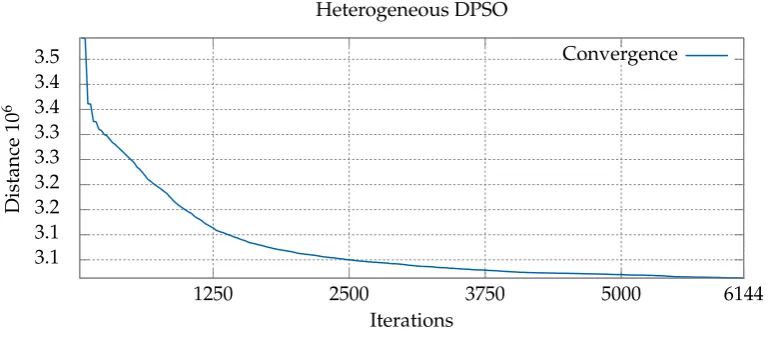
interval. Table4presents the results, while Figure 6shows the speed of convergence towards an 257
optimum in each phase. As can be seen, different sets of parameter values dominate subsequent phases 258
(intervals) of the computations. In the first interval (0–1250), the sets with small parameter values 259
are predominant—which indicates that rapid changes in the particle solutions are beneficial. In the 260
third interval (2500–3750), the sets of parameter values are mixed, i.e. they contain both small and 261
high values. This can be interpreted as a sign that the exploration of the solution space slows down 262
and, more importantly, becomes exploitation. In the last interval (5000–6144), the best particles have 263
relatively high parameter values, which, combined with stronger pheromone reinforcement, causes 264
mainly small changes to the particle positions. 265
6.2. Comparative Study 266
To evaluate the performance of the proposed DPSO algorithm, we have compared it with the 267
homogeneous version of the DPSO and with ACS and PACO, which are among the best-performing 268
metaheuristics for the TSP and DTSP problems. The DTSP test instances were generated based on the 269
Table 4.Ranking of parameter values for which the particles in the heterogeneous DPSO were able to improve the global best solution the greatest number of times within four designed subsequent phases of the computations. The results are accumulated over 30 executions for thegr666TSP instance.
Iterations Parameters Number ofgBestimprovements c1 c2 c3 ω
0–1250
0.1 0.1 0.1 0.1 94
0.1 0.1 0.1 0.5 93
0.1 2 2 0.5 38
0.1 2 0.1 0.1 38
0.1 2 2 0.1 32
1250–2500
0.75 2 2 0.25 12
1.5 2 0.1 0.1 10
0.1 2 0.1 0.1 10
0.1 1.5 0.1 0.5 9
0.1 1 2 0.1 8
2500–3750
0 .1 0.1 0.1 0.5 10
1.5 1.5 2 0.5 4
1.5 2 0.1 0.25 4
0.75 2 2 0.25 3
0.1 1 2 0.1 3
3750–5000
0.1 1 0.1 0.1 2
0.1 1 2 0.1 2
0.75 0.1 2 0.5 2
1.5 0.1 2 0.1 2
1.5 2 1.5 0.1 2
5000–6144
1.75 2 1 0.5 3
1.5 2 1.5 0.1 2
1.75 0.1 2 0.5 2
0.1 1.5 0.1 0.5 2
3.1 3.1 3.2 3.2 3.3 3.3 3.4 3.4 3.5
1250 2500 3750 5000 6144
Distance
10
6
Iterations Heterogeneous DPSO
Convergence
Figure 6.Chart showing convergence with the optimum of the heterogeneous version of the algorithm for thegr666problem.
repository.1Algorithm1presents an outline of the general test procedure used to solve the DPSO with 271
the algorithms mentioned. 272
Algorithm 1Outline of the procedure for solving the DTSP.
Load the static TSP instance .The original TSP instance becomes the first DTSP sub-problem Initialize the algorithm-related data
whileStop criterion is not metdo
sub-problem-related initialization .Create swarm and neighbourhood etc.
Solve the current sub-problem .Solve with DPSO, ACO, etc.
Modify the current sub-problem to obtain the next one end while
To make the comparison fair, all algorithms were solving the same DTSP instances, i.e. starting 273
from the same static TSP and including the same DTSP-related changes to the positions of the cities. 274
Each DTSP instance comprised 11 static TSP sub-problems, namely the original problem from TSPLIB 275
and ten sub-problems resulting from random changes to the position of the cities. Thegr666problem 276
was an exception, since it included only one sub-problem (the original TSPLIB problem). Figure7 277
shows an example of a DTSP instance consisting of two static TSP sub-problems. 278
Table5shows the parameter values of the two DPSO variants. The numbers of iterations used are 279
shown alongside the results in Table6. The size of the swarm and the size of the particle neighbourhood 280
were determined from preliminary computations, keeping in mind that both parameters strongly 281
influence the computation time and the quality of the solutions. A smaller neighbourhood limits 282
the solution space and speeds up computation. However, too low a value could hamper finding the 283
optimum. The parameters (c1,c2,c3,ω,SwarmSize, andneighbourhood) for thehomogeneousversion of
284
the DPSO were chosen based on preliminary computations and our previous work on DPSO. 285
The ACS and PACO parameters were set as follows: number of ants = 10; number of iterations = 286
b0.1·pevc;β=3; local and global pheromone evaporation coefficientsα=0.1 andρ=0.1, respectively;
287
andq0= (n−10)/n, wherenis the size of the problem. For the PACO algorithm,q0=0.8 was used 288
and theage-basedstrategy for updating the solution archive (of size 5) was used. The values of the 289
parameters were set based on preliminary computations and the suggestions by Cáceres el al. [27], in 290
which the ACO was tested with a small computation budget. 291
Figure 7.Visualization of the optimum routes for the statickroA100TSP instance (left side) and the DTSP instance after a random relocation of some cities (right side). The edges differentiating the new optimum from the previous are marked in red.
All the considered algorithms, including DPSO and ACO, were allowed to construct and evaluate 292
exactly the same number of solutions (pev) to a problem. For example, the DPSO algorithm with 104
293
iterations and a swarm of size 32 constructed a total ofpev=104·32=3328 solutions. All algorithms
294
were implemented in the C# language and run on a computer with an Intel i7 3.2 GHz CPU. All 295
computations were repeated 30 times and the results were averaged. 296
Table 5.Values of DPSO-related parameters.
Homogeneous DPSO Heterogeneous DPSO Common parameters
Problem c1 c2 c3 ω Problem c1 c2 c3 ω SwarmSize Neighbourhood
berlin52 0.5 0.5 0.5 0.2 berlin52, kroA100, kroA200, gr202,
gr666
Chosen randomly as described in Sec.5
32 7
kroA100 0.5 0.5 0.5 0.5 64 7
kroA200 0.5 0.5 0.5 0.5 80 7
gr202 0.5 0.5 0.5 0.5 101 10
gr666 0.5 1.0 1.5 0.6 112 30
For the smallest DTSP instance (berlin52), both DPSO versions generated results that were 297
of similar quality and, at the same time, better than those of the ACO algorithms. For the larger 298
instances, the heterogeneous DPSO shows a clear advantage over the homogeneous DPSO. The biggest 299
differences were observed for thepcb442andgr202instances, for which the heterogeneous version 300
generated higher-quality solutions, especially if the number of iterations was low. This confirms that 301
the heterogeneity of the parameter values results in a broader exploration of the solution search space. 302
At the same time, the heterogeneous DPSO is also more consistent in finding high-quality solutions, 303
which is manifested in the smaller average standard deviation compared with the homogeneous 304
version. When the number of iterations grows, the advantage of the heterogeneous DPSO becomes 305
less—confirming that, in the later stages of the computations, the exploitative nature of the algorithm 306
becomes more important. Generally, both DPSO versions benefit from a larger number of iterations. 307
Compared with the ACO algorithms, the DPSO variants converge more rapidly and the increasing 308
number of iterations allows them to outperform ACS and PACO in almost all cases. 309
7. Conclusions 310
We have proposed a heterogeneous DPSO algorithm for solving the DTSP. In this algorithm, each 311
particle can have different values of the crucial DPSO parametersc1,c2,c3, andω. These values are
312
chosen randomly according to the discrete probability distribution defined so that different behaviours 313
of the DPSO particles can be obtained. Computational experiments conducted on a set of DTSP 314
instances have shown that it is beneficial if some particles explore the solution space while others are 315
Table 6. Comparison of results for the homo- and heterogeneous DPSO variants and the ACO algorithms obtained for four DTSP (berlin52,. . ., pcb442) and one TSP (gr666) instances. “G” denotes the distance to the optimum and “D” the average standard deviation of this distance. The numbers of iterations are given per sub-problem. The best solutions found by the DPSO algorithms are marked in boldface.
Problem Iterations
DPSO algorithms Counterparts
Homogeneous Heterogeneous ACS PACO
T [s] G [%] D [%] T [s] G [%] D [%] G [%] G [%] berlin52 104 0.13 0.15 0.32 0.13 0.13 0.15 0.96 0.96 berlin52 416 0.3 0.01 0.04 0.28 0.01 0.05 0.5 0.5 berlin52 1664 0.98 0 0 0.89 0.01 0.05 0.46 0.46 kroA100 100 1.03 5.44 2.47 0.86 2.68 1.4 1.8 2.97 kroA100 400 1.63 1.28 1.02 1.27 1.05 0.81 1.31 2.13 kroA100 1600 4.11 0.64 0.69 3.38 0.78 0.77 0.82 1.36 kroA200 160 2.49 15.63 2.77 2.18 5.14 1.84 2.41 3.33 kroA200 640 5.13 4.45 1.62 4.46 2.89 1.09 1.62 2.71 kroA200 2560 15.6 1.62 0.81 13.18 2.02 0.8 1.47 2.28 gr202 128 8.82 13.75 2.06 8.17 4.19 1.2 6.26 4.91 gr202 512 11.54 6.81 2.11 10.88 1.97 0.66 4.88 3.9 gr202 2048 23.01 1.52 0.6 21.98 1.53 0.55 3.93 3.34 pcb442 272 11.22 29.31 5.33 11.16 6.73 1.68 6.18 4.44 pcb442 1088 28.52 13.41 5 30.69 2.87 0.89 4.87 3.56 pcb442 4352 102.78 3.13 1.52 108.25 1.92 0.79 3.91 3.3
gr666 384 85.19 10.84 1.52 91.83 9.58 0.86 9.18 5.89 gr666 768 98.36 7.37 1.0 115.19 6.88 0.78 7.46 4.77 gr666 1536 124.84 5.62 0.84 163.48 5.33 0.57 6.09 4.51 gr666 3072 180.66 4.88 0.63 259 4.52 0.88 5.67 4.14 gr666 6144 296.83 3.99 0.77 453.83 3.8 0.78 4.92 4.21
found so far. The heterogeneous DPSO algorithm improves the quality of the results obtained compared 317
with the homogeneous version. Moreover, the algorithm is easier to use, since fewer parameters have 318
to be set manually, which is important because choosing the right values of the parameters can be 319
especially difficult for the DTSP. It is also worth emphasizing that both versions of the DPSO algorithm 320
are comparable to the proven ACS and PACO metaheuristics in terms of solution quality. In fact, 321
heterogeneous DPSO is able to generate solutions of better quality than both of ACO-based algorithms 322
in most cases, while also exhibiting more rapid convergence if the computation time is extended. 323
In the future, we plan to test different types of heterogeneity in addition to the parameter diversity 324
considered here. 325
Author Contributions:Conceptualization, Łukasz Str ˛ak, Rafał Skinderowicz, Urszula Boryczka and Arkadiusz 326
Nowakowski; Formal analysis, Łukasz Str ˛ak, Rafał Skinderowicz and Urszula Boryczka; Investigation, Łukasz 327
Str ˛ak, Rafał Skinderowicz, Urszula Boryczka and Arkadiusz Nowakowski; Methodology, Łukasz Str ˛ak, Rafał 328
Skinderowicz, Urszula Boryczka and Arkadiusz Nowakowski; Project administration, Łukasz Str ˛ak and Rafał 329
Skinderowicz; Resources, Łukasz Str ˛ak and Rafał Skinderowicz; Software, Łukasz Str ˛ak and Rafał Skinderowicz; 330
Supervision, Łukasz Str ˛ak and Rafał Skinderowicz; Validation, Łukasz Str ˛ak and Rafał Skinderowicz; Visualization, 331
Łukasz Str ˛ak and Rafał Skinderowicz; Writing – original draft, Łukasz Str ˛ak, Rafał Skinderowicz and Urszula 332
Boryczka; Writing – review & editing, Łukasz Str ˛ak, Rafał Skinderowicz and Urszula Boryczka. 333
Conflicts of Interest:The authors declare no conflict of interest. 334
Abbreviations 335
The following abbreviations are used in this paper: 336
ACO ant colony optimization
DPSO discrete particle swarm optimization DTSP dynamic travelling salesman problem PACO population ant colony optimization PSO particle swarm optimization TSP travelling salesman problem 338
References 339
1. Branke, J. Evolutionary approaches to dynamic environments. In GECCO Workshop on Evolutionary 340
Algorithms for Dynamics Optimization Problems2001. 341
2. Li, W. A parallel multi-start search algorithm for dynamic traveling salesman problem. International 342
Symposium on Experimental Algorithms. Springer, 2011, pp. 65–75. 343
3. Kennedy, J.; Eberhart, R. Particle Swarm Optimization.In Proceedings of the IEEE International Conference on 344
Neural Networks1995, pp. 1942–1948. 345
4. Kennedy, J.; Eberhart, R.C. A discrete binary version of the particle swarm algorithm. Systems, Man, and 346
Cybernetics, 1997. Computational Cybernetics and Simulation., 1997 IEEE International Conference on, 347
1997, Vol. 5, pp. 4104–4108 vol.5. 348
5. Clerc, M. Discrete Particle Swarm Optimization, illustrated by the Traveling Salesman Problem. InNew 349
Optimization Techniques in Engineering; Springer Berlin Heidelberg, 2004; Vol. 141,Studies in Fuzziness and 350
Soft Computing, pp. 219–239. 351
6. Shi, X.H.; Liang, Y.C.; Lee, H.P.; Lu, C.; Wang, Q. Particle swarm optimization-based algorithms for TSP 352
and generalized TSP.Information Processing Letters2007,103, 169–176. 353
7. liang Zhong, W.; Zhang, J.; neng Chen, W. A Novel Set-Based Particle Swarm Optimization Method for 354
Discrete Optimization Problems. InEvolutionary Computation, 2007. CEC 2007; IEEE, 1997; Vol. 14, pp. 355
3283–3287. 356
8. Str ˛ak, Ł.; Skinderowicz, R.; Boryczka, U. Adjustability of a discrete particle swarm optimization for the 357
dynamic TSP.Soft Computing2018,22, 7633–7648. 358
9. Hansell, M.Built by Animals; Oxford University Press: New York, 2007. 359
10. Nepomuceno, F.V.; Engelbrecht, A.P. A Self-adaptive Heterogeneous PSO Inspired by Ants. InSwarm 360
Intelligence; Springer Berlin Heidelberg, 2012; Vol. 7461,Lecture Notes in Computer Science, pp. 188–195. 361
doi:10.1007/978-3-642-32650-9_17. 362
11. Montes de Oca, M.A.; Peña, J.; Stützle, T.; Pinciroli, C.; Dorigo, M. Heterogeneous Particle Swarm 363
Optimizers. InIEEE Congress on Evolutionary Computation (CEC 2009); Haddow, P.; others., Eds.; IEEE Press: 364
Piscatway, NJ, 2009; pp. 698–705. 365
12. Boryczka, U.; Str ˛ak, L. Heterogeneous DPSO Algorithm for DTSP. InComputational Collective Intelligence; 366
Núñez, M.; Nguyen, N.T.; Camacho, D.; Trawi ´nski, B., Eds.; 2015; Vol. 9330,Lecture Notes in Computer 367
Science, pp. 119–128. 368
13. Psaraftis, H. Dynamic vehicle routing problems.Vehicle routing: Methods and studies1988,16, 223–248. 369
14. Li, C.; Yang, M.; Kang, L. A new approach to solving dynamic traveling salesman problems. Proceedings of 370
the 6th international conference on Simulated Evolution And Learning; Springer-Verlag: Berlin, Heidelberg, 371
2006; SEAL’06, pp. 236–243. 372
15. Cook, W.J.In pursuit of the traveling salesman: mathematics at the limits of computation; Princeton University 373
Press, 2011. 374
16. Guntsch, M.; Middendorf, M. Pheromone Modification Strategies for Ant Algorithms Applied to Dynamic 375
TSP. InApplications of Evolutionary Computing; Springer Berlin Heidelberg, 2001; Vol. 2037,Lecture Notes in 376
Computer Science, pp. 213–222. 377
17. Eyckelhof, C.J.; Snoek, M. Ant Systems for a Dynamic TSP. InAnt Algorithms; Springer Berlin Heidelberg, 378
2002; Vol. 2463,Lecture Notes in Computer Science, pp. 88–99. 379
18. Helsgaun, K. An Effective Implementation of the Lin-Kernighan Traveling Salesman Heuristic.European 380
19. Mavrovouniotis, M.; Yang, S. Ant Colony Optimization with Immigrants Schemes in Dynamic 382
Environments. InParallel Problem Solving from Nature, PPSN XI; Springer Berlin Heidelberg, 2010; Vol. 6239, 383
Lecture Notes in Computer Science, pp. 371–380. 384
20. Simões, A.; Costa, E. CHC-Based Algorithms for the Dynamic Traveling Salesman Problem. InApplications 385
of Evolutionary Computation; Springer Berlin Heidelberg, 2011; Vol. 6624,Lecture Notes in Computer Science, 386
pp. 354–363. 387
21. Younes, A.; Basir, O.; Calamai, P. A Benchmark Generator for Dynamic Optimization. Proceedings of 388
the 3rd WSEAS International Conference on Soft Computing, Optimization, Simulation & Manufacturing 389
Systems, 2003. 390
22. Tinós, R.; Whitley, D.; Howe, A. Use of Explicit Memory in the Dynamic Traveling Salesman Problem. 391
Proceedings of the 2014 Annual Conference on Genetic and Evolutionary Computation; ACM: New York, 392
NY, USA, 2014; GECCO ’14, pp. 999–1006. 393
23. Zhang, Y.; Zhao, G., Research on Multi-service Demand Path Planning Based on Continuous Hopfield 394
Neural Network. InProceedings of China Modern Logistics Engineering: Inheritance, Wisdom, Innovation and 395
Cooperation; Springer Berlin Heidelberg: Berlin, Heidelberg, 2015; pp. 417–430. 396
24. Eaton, J.; Yang, S.; Mavrovouniotis, M. Ant colony optimization with immigrants schemes for the 397
dynamic railway junction rescheduling problem with multiple delays.Soft Computing2016,20, 2951–2966. 398
doi:10.1007/s00500-015-1924-x. 399
25. Mavrovouniotis, M.; Shengxiang, Y. Empirical study on the effect of population size on MAX-MIN ant 400
system in dynamic environments. 2016 IEEE Congress on Evolutionary Computation (CEC), 2016, pp. 401
853–860. doi:10.1109/CEC.2016.7743880. 402
26. Mavrovouniotis, M.; Müller, F.M.; Shengxiang, Y.M.M. Ant Colony Optimization With Local Search 403
for Dynamic Traveling Salesman Problems. IEEE Transactions on Cybernetics 2017, 47, 1743–1756. 404
doi:10.1109/TCYB.2016.2556742. 405
27. Cáceres, L.P.; López-Ibánez, M.; Stützle, T. Ant colony optimization on a budget of 1000. InSwarm 406