High-speed Receiver Behavioral Modeling Using Machine Learning.

(1)

LI, BOWEN. High-speed Receiver Behavioral Modeling Using Machine Learning. (Under the direction of Dr. Paul D. Franzon).

In the high-speed Serializer/Deserializer (SerDes) application, with the rising frequencies,

signal integrity analysis becomes challenging. To simulate the performance of the SerDes link,

behaviors of the transceiver need to be modeled accurately. In this research, we focus on the

high-speed receiver behavioral modeling.

Nowadays, the IBIS-AMI model becomes the most efficient simulation model for the

high-speed SerDes simulation. The IBIS-AMI model can finish one simulation in about 30 minutes for

each channel. After the simulation, users can get the transient simulation results, namely transient

waveform, eye diagram and bathtub curve, and adaptation simulation results, such as CTLE and

DFE settings at the receiver.

However, the IBIS-AMI model can only do adaptation and transient simulation at the same

time, which would be inefficient in two scenarios. The first scenario is that users only want to get

transient simulation results under one receiver setting to see the eye-opening or bathtub curve

information. The second scenario is that users only want to know the receiver adaptation codes,

which can represent the equalization status of the SerDes link. In both scenarios, people have to

wait for 30 minutes and get some redundant simulation results. In that case, individual behavioral

models need to be built for these two receiver simulations, while the simulation speeds of the

models should be faster than the IBIS-AMI model.

In this research, as for the transient behavioral modeling, we propose a method, called

adaptive-ordered system identification model, to simulate the transient simulation results of the

(2)

eye diagram, and bathtub curve predictions.

As for the adaptation behavioral modeling, we propose a Cascaded Deep Learning (CDL)

modeling mechanism to show a parallel approach to modeling adaptive SerDes behavior

effectively. Specifically, the proposed modeling methodology uses a cascaded deep learning model

structure to predict the receiver adaptation codes. The modeling method shows high correlations

with the real adaptation results. Meanwhile, this modeling mechanism has good scalability, which

can learn adaptation behaviors from various SerDes designs.

For the simulation speed, the proposed adaptive-ordered system identification model and

(3)

(4)

by Bowen Li

A dissertation submitted to the Graduate Faculty of North Carolina State University

in partial fulfillment of the requirements for the degree of

Doctor of Philosophy

Computer Engineering

Raleigh, North Carolina 2020

APPROVED BY:

_______________________________ _______________________________ Paul D. Franzon Brian Floyd

Committee Chair

(5)

ii

DEDICATION

(6)

iii

BIOGRAPHY

Bowen Li was born in December 1991, Shijiazhuang, Hebei, China. He received his

bachelor’s degree from Beijing University of Posts and Telecommunications in June 2014 and his

master’s degree from North Carolina State University in May 2018. In August 2015, he started his

graduate research work with Dr. Paul Franzon in the area of machine learning in Electronic design

automation (EDA) in North Carolina State University. During his Ph.D., he interned at Hewlett

Packard Enterprise and Samsung. His research topic is high-speed receiver behavioral modeling

(7)

iv

ACKNOWLEDGMENTS

I want to express my sincere gratitude to my research advisor, Dr. Paul Franzon, for his

guideline, understanding and support. I also want to thank him for introducing me to the machine

learning related research topic and providing me the opportunity to join the CAMEL center.

Furthermore, I want to thank my committee member, Dr. Brian Floyd, Dr. Rhett Davis and Dr.

Min Chi for insightful advice and understanding during the research work.

I’m also grateful to the following people and organizations, without whom I could not have

made this accomplishment. These include Dr. Brandon Jiao, who inspired me in the SerDes design

area and helped me during my research; Dr. Yongjin Choi, who was the mentor during my very

first internship in my life; my group fellows Weiyi Qi, Sumon Dey, Weifu Li, Jong Beom Park,

Zhao Wang, Bill Huggins, Yi Wang, and Luis Francisco, Yuejiang Wen, who have made special

pieces of the beautiful memory of the past years; and my friends from other research groups Junyu

Shen, Yuan Chang, Ruonan Yang, who support me during my Ph.D. research.

Finally, I would like to give my most sincere gratefulness to my parents. Their love and

(8)

v

LIST OF TABLES

Table 4.1. Avago transceiver setting configuration ... 31

Table 4.2. UltraScale+ GTY transceiver setting configuration ... 40

Table 4.3. Training and testing data configuration for CTLE mode and DFE mode ... 48

Table 4.4. Eye margin prediction results for CTLE mode ... 52

Table 4.5. Bathtub curve prediction results for CTLE mode ... 52

Table 4.6. Eye margin prediction results for DFE mode ... 56

Table 4.7. Bathtub curve prediction results for DFE mode ... 56

Table 4.8. Cross-validation results for CTLE and DFE mode ... 57

Table 4.9. Performance comparison between the LSTM and proposed ANNARX model ... 58

Table 5.1. Data configuration for two transceiver designs ... 66

Table 5.2. Prediction results using one LSTM model ... 69

Table 5.3. Prediction results using DNN + LSTM model ... 74

Table 5.4. Best model configurations for the proposed modeling mechanism ... 76

Table 5.5. Prediction results using the CDL model ... 78

(11)

viii

LIST OF FIGURES

Figure 2.1. High-Speed Electrical Link with Equalization Schemes ... 9

Figure 2.2. CTLE effect illustration ... 10

Figure 2.3. CTLE circuit structure ... 11

Figure 2.4. Basic DFE working mechanism ... 12

Figure 2.5. DFE tap function ... 13

Figure 2.6. Typical eye diagrams after DFE ... 13

Figure 2.7. IBIS-AMI simulation description ... 15

Figure 2.8. Linear system identification configuration ... 16

Figure 2.9. NNARX structure ... 18

Figure 2.10. Deep Neural Networks structure ... 20

Figure 2.11. RNN unfolded topological graph ... 22

Figure 2.12. LSTM cell structure ... 22

Figure 4.1. Data measurement from the 10 Gbps Avago transceiver ... 31

Figure 4.2. Linear system identification model performance ... 34

Figure 4.3. Nonlinear system identification model performance ... 35

Figure 4.4. LSTM model performance ... 35

Figure 4.5. Model performances for 50 cases ... 36

Figure 4.6. NNARX model training and prediction process ... 39

Figure 4.7. Two signal integrity analysis methods ... 42

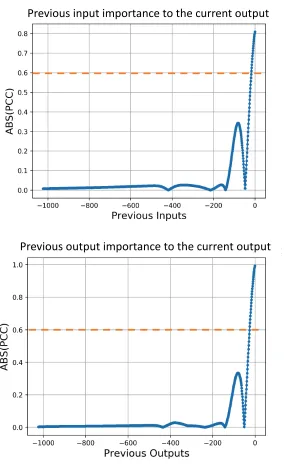
Figure 4.8. PCC scores of previous inputs and outputs for the current output ... 44

Figure 4.9. Adaptive-ordered system identification model structure ... 45

Figure 4.10. Receiver equalized transient modeling process chart ... 47

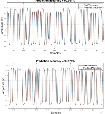
Figure 4.11. Waveform prediction results using the ANNARX model in CTLE mode ... 49

Figure 4.12. Real vs prediction eye diagram comparison in CTLE mode ... 50

Figure 4.13. Real vs prediction bathtub curve comparison in CTLE mode ... 51

Figure 4.14. Waveform prediction results using the ANNARX model in DFE mode ... 53

Figure 4.15. Real vs prediction eye diagram comparison in DFE mode ... 54

Figure 4.16. Real vs prediction bathtub curve comparison in DFE mode ... 55

Figure 4.17. Receiver setting recommendation ... 59

Figure 5.1. Traditional IBIS-AMI model vs CDL model in the receiver adaptation simulation .. 61

Figure 5.2. Data collection process ... 64

Figure 5.3. Three-stage CTLE in UltraScale+ GTH and GTY transceiver ... 65

Figure 5.4. Adaptation process for one receiver code ... 68

Figure 5.5. Adaptation code prediction using the LSTM model ... 68

Figure 5.6. Low-frequency and high-frequency signal amplitude measurement ... 70

Figure 5.7. DFE cancellation region ... 70

Figure 5.8. Sliced SBR data as the input of LSTM model ... 71

Figure 5.9. DNN + LSTM modeling mechanism ... 72

Figure 5.10. Cascaded Deep Learning modeling mechanism ... 75

Figure 5.11. CTLE code (AGC, KL, and KH) prediction results in the UltraScale+ GTY ... 79

Figure 5.12. DFE Tap (DFE Tap1 - 4) prediction results in the UltraScale+ GTY ... 82

Figure 5.13. CTLE adaptation code (AGC, KL, KH) prediction in UltraScale+ GTH receiver ... 86

Figure 5.14. DFE tap1- 4 predictions in UltraScale+ GTH receiver ... 89

(12)

(13)

1

Chapter 1. Introduction

With the increasing data rate and distance of the wireline communication system, signal

integrity analysis becomes challenging in high-speed Serializer-Deserializer (SerDes) links. The

performance of the SerDes link needs to be analyzed and simulated efficiently. To analyze and

simulate the performance of the entire SerDes link, behaviors of the transmitter (TX) and receiver

(RX) need to be accurately modeled. In the SerDes link simulation, the most challenge part is to

build a receiver behavioral model. Nowadays, because of the low target serial link error rate, for

example, 1e-15, the existing simulation tools, like SPICE simulation, and traditional IBIS model,

cannot provide fast and accurate simulations.

In that case, the IBIS Algorithmic Modeling Interface (IBIS-AMI) model is proposed [15]

[33]. The IBIS-AMI model is a powerful method to incorporate SerDes and channel models into

a unified simulation environment that protects vendors’ intellectual property (IP) [19]. The

IBIS-AMI is a behavior model, which is generated by the semiconductor vendors and for the customers

to do the simulation. However, the IBIS-AMI model can only do adaptation and transient

simulation at the same time, which would be inefficient in some situations. And the simulation

speed of the IBIS-AMI model is 30 minutes for each run. Hence, we need to find a way to build

behavioral models for these two simulations separately, while the performance of the behavioral

models should be better than the IBIS-AMI model.

In this work, we focus on modeling the receiver behavior using machine learning methods,

which can provide fast and high-precision simulation. Two behavioral models are built for these

(14)

2

1.1. Motivation

In the transceiver or SerDes industry, there is one efficient way to do the transceiver

simulation, which is the IBIS-AMI model. The IBIS-AMI model is a behavior model and shows a

high correlation with the on-die circuit. The IBIS-AMI model can do signal integrity analysis in

about 30 minutes for each channel. After the simulation, users can get the equalized transient

simulation results, namely transient waveform, eye diagram and bathtub curve, and adaptation

simulation results, such as adaptation codes at the receiver. However, the IBIS-AMI model can

only do adaptation and transient simulation at the same time, which would be inefficient in two

scenarios. The first scenario is that users want to get transient simulation results to see the

eye-opening or bathtub curve information. The second scenario is that users only need to know the

receiver adaptation codes, which represent the equalization status of the SerDes link. In that case,

we need to find a way to build behavioral models for these two simulations separately, while the

performance of the behavioral models should be the same or better than the IBIS-AMI model.

Recently, some works have been done in high-speed receiver behavioral modeling to

speedup post-silicon validation. Those related work can be divided into two research areas. The

first area is to predict eye-opening using machine learning models. Neural networks (NN) [12] or

support vector machine (SVM) [28] [29] are trained to predict the eye height and eye width after

the receiver equalization using the circuit features. However, those methods are grey-box modeling,

which needs to know the inner structure of the circuit. In a SerDes system, there are approximately

thousands of circuit features impacting the recovered signal in SerDes receiver. The published

grey-box methods take a couple out of the thousands of features to build the ML model and do

(15)

3 receiver output waveforms according to the receiver input waveforms. Those methods are

black-box modeling, which doesn’t need any internal information of the circuit.

For the published gray-box modeling, the tradeoff is the more features adopted in the ML

model the more accurate the prediction but the model complexity and simulation time increase.

The accuracy of the grey-box method will be sacrificed to balance the model complexity as well

as simulation time. What’s more, the gray-box modeling methods can only predict eye height and

width, which is only a small part of the whole picture of the equalized signal inside the receiver.

For the published black-box modeling, there are no modeling methods which can only train the

model once and predict the transient waveforms, not from the same training pseudorandom binary

sequence (PRBS) data and training channel. Moreover, some publications provide prediction

accuracy while some do not. The provided accuracy numbers are all about eye height and eye

width prediction without giving the accuracy number for predicted transient waveforms. Besides,

no publications are found to do bathtubs prediction. The bathtub prediction is based on the eye

diagram constructed from long enough transient waveforms. Generally, it needs about a million

bits. The ML model complexity determines the model prediction/simulation time and consequently,

the total length of the transient waveform prediction can be obtained with reasonable simulation

time. All the latest published work can predict much fewer bits required for bathtub prediction.

The proposed modeling method in this work can predict long bits in a short time and shows a

high-precision prediction of the transient waveform, eye diagram, and bathtub. The proposed modeling

method is a black-box modeling approach and provides a fast and high-precision, which can train

the model once and predict transient waveforms, eye diagram and bathtub curve using different

PRBS data patterns and different channels. The black-box method does not consider any SerDes

(16)

4 limited by SerDes circuit details. To meet all the functions in the receiver, the

machine-learning-based receiver model can provide transient waveform, eye diagram, and bathtub curve predictions

at the same time.

The receiver adaptation process is another important feature in the high-speed transceiver

simulation. In the transceiver or SerDes industry, there is only one way in the modeling method,

called the IBIS-AMI model, to give the users the adaptation results, which is a part of the IBIS

standard. However, the simulation speed of the adaptation process is very time-consuming. If the

transmitter (TX) or the channel is changed, engineers have to wait for a half-hour to see the

adaptation results using the IBIS-AMI model. Moreover, designing an IBIS-AMI model needs

detailed information about the circuit design and lots of trials and errors to improve model

performance. Currently, no research focuses on equalization adaptation modeling using machine

learning technique.

In this research, machine learning (ML) models are used to predict equalized results,

namely transient waveforms, eye diagrams, and bathtub curves, and the adaptation codes using the

receiver input waveforms. The design and simulation process of the proposed modeling methods

are much faster than the IBIS-AMI model.

1.2. Contribution

In this work, an adaptive-ordered system identification model is proposed for the receiver

equalized result prediction. The main contributions of the proposed modeling method can be

summarized as below:

1. Self-adaptive model complexity. The proposed modeling method can quickly predict

(17)

5 2. The proposed model can provide transient waveform, eye diagram, and bathtub curve

simulation at the same time.

3. No re-train is needed to predict over various channels and no accuracy degradation when

changing the data pattern, transmitter settings, and channels.

4. Fast training and prediction time compared to existing modeling methods. The

simulation speed is much faster than the IBIS-AMI model.

The Cascaded Deep Learning (CDL) modeling mechanism is proposed to show a parallel

approach to modeling adaptive SerDes behavior effectively. The main contributions of the CDL

modeling method in this work can be summarized as below:

1. Originality. No previous work focuses on the SerDes receiver adaptation modeling using

a machine learning approach.

2. The modeling mechanism can do cascaded prediction.

3. The proposed model provides high-precision receiver adaptation simulation results.

4. The simulation speed is much faster than the IBIS-AMI model.

5. Good scalability. This modeling mechanism can learn adaptation behaviors from

different SerDes designs.

1.3. Organization

We organize the rest as follows. Chapter 2 introduce the fundamentals of the SerDes link,

and the machine learning models we used. In Chapter 3, we obtain the related state-of-arts research

on the high-speed receiver behavioral modeling and compare those work with our proposed

method.

Chapter 4 proposes the adaptive-ordered system identification modeling method for the

(18)

6 Chapter 5 presents the CDL modeling mechanism for receiver adaptation behavior. We

will compare the results with the on-die circuit adaptation codes.

Chapter 6 concludes the work we’ve done for the high-speed receiver behavioral modeling

and discusses the potential future work.

1.4. Abbreviations

SerDes Serializer-Deserializer

TX Transmitter

RX Receiver

LTI linear time-invariant

IBIS Input/output Buffer Information Specification

IBIS-AMI IBIS Algorithmic Modeling Interface

NN Neural network

SVM Support Vector Machine

ISI Inter-symbol interference

CTLE continuous time linear equalizer

DFE decision feedback equalizer

FFE feed-forward equalization

AGC auto gain control

SNR signal noise ratio

UI Unit interval

PCB Printed Circuit Board

ARX AutoRegressive eXternal input

ARMAX AutoRegressive Moving Average eXternal input

MLP Multilayer perceptron

(19)

7

ReLU Rectified linear unit

SGD Stochastic gradient descent

LSTM Long short-term memory

RNN Recurrent neural networks

VRNN Vanilla RNN

ANN Artificial Neural Networks

BER Bit error rate

LMS least mean square

NRMSA Normalized root mean square accuracy

100GE 100 Gigabit Ethernet

KH High-frequency gain

KL Low-frequency gain

VSR Very short reach

SR Short reach

MR Medium reach

BERT Bit error ratio testers

DUT Device under test

PDF Probability density function

DJ Deterministic jitter

RJ Random jitter

ML Machine learning

NNARX ARX model based on neural networks

ANNARX Adaptive-ordered NNARX

PCC Pearson Correlation Coefficient

(20)

8

HDL Hardware description language

CDL Cascaded Deep Learning

IP Intellectual property

PVT Process, voltage, and temperature

PRBS Pseudorandom binary sequence

SBR Single bit response

LPR Long pulse response

MSE Mean square error

PTL Predicted target library

CNN convolutional neural networks

(21)

9

Chapter 2. Background and Fundamentals

In this chapter, we will describe the fundamentals of the SerDes link, IBIS-AMI model,

and machine learning models used in this research.

2.1. SerDes Background

Signal integrity analysis becomes challenging in high-speed SerDes links. A basic SerDes

link has a transmitter (TX), a channel, and a receiver (RX). The receiver consists of a continuous

time linear equalizer (CTLE) and a decision feedback equalizer (DFE), which are used to mitigate

inter-symbol interference (ISI). An ideal cable could propagate all frequency contents without any

loss. TX feed-forward equalization (FFE) acts as a FIR filter and pre-distorts transmitted pulse in

order to invert channel distortion. At receiver side, RX CTLE and DFE are implemented as part of

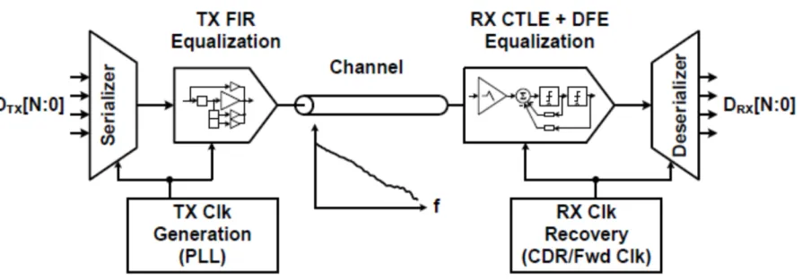
receiver circuits and flatten the system response through conditioning the receiving signal. Figure

2.1 shows a high-speed electrical link using TX FFE equalization and RX CTLE+DFE

equalization.

Figure 2.1. High-Speed Electrical Link with Equalization Schemes

We will briefly introduce the TX technology and talk about CTLE and DFE technology

(22)

10 implemented through a FIR filter. It pre-distorts or shapes the data over several bit periods in order

to invert the channel loss/distortion. The low frequency contents get de-emphasized in order to

flatten the channel response. The advantages of the TX are: 1) High speed DAC is relatively easy

to implement compared with receiver high speed ADC; 2) TX FFE can cancel pre-cursor ISI; 3)

Due to the digital nature of the TX FFE, the noise is not amplified. The disadvantages are: 1) To

flatten the channel response, low frequency content is attenuated due to the peak-power limitation.

2) To tune the FIR taps, a feedback path from receiver side is required to detect channel response.

Next, CTLE and DFE technology are introduced.

2.1.1. Basics of CTLE

CTLE, also known as linear equalizer, filters RX input signal by relatively attenuating the

low frequency content and boosting high frequency content attenuated through the channel. It

introduces zeros to offset the frequency-dependent channel loss. Generally, the CTLE is preceded

and followed by an auto gain control (AGC) circuit to bring the signal to the appropriate level to

achieve acceptable signal noise ratio (SNR) and to not amplify the signal too much to go too much

beyond the nonlinear range. While boosting high frequency signal, CTLE could potentially

amplify noise and crosstalk depending on the required CTLE settings. This calls for more

precautions in using CTLE for certain applications, for example, when the environment is noisy.

An example of CTLE effect in reducing channel ISI is illustrated in Figure 2.2 [24].

(23)

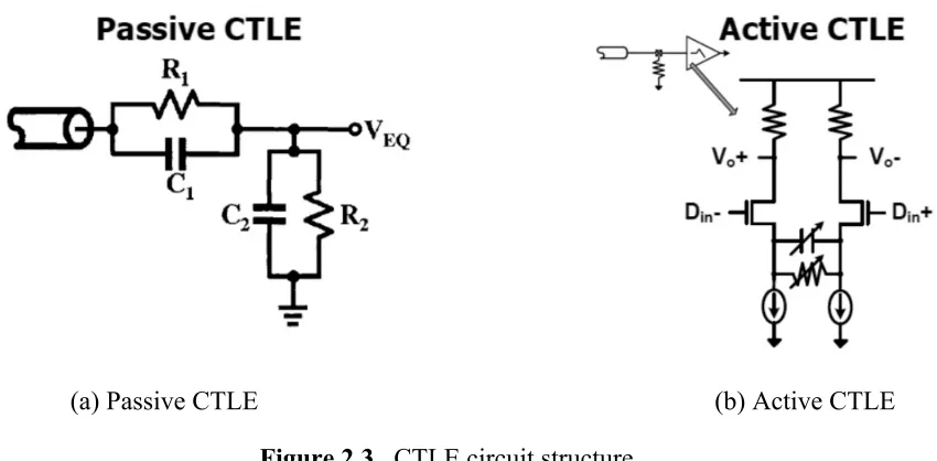
11 CTLE can be divided into two types, passive [22] and active filter [23]. Both passive and

active filter can realize high-pass transfer function to compensate for the channel loss as shown in

Figure 2.3. Both pre-cursor and long-tail ISI can be cancelled using the linear equalizer.

(a) Passive CTLE (b) Active CTLE

Figure 2.3. CTLE circuit structure

The passive CTLE is the combination of passive low pass filter and high pass filter. Active

CTLE can be implemented through a differential pair with RC degeneration with gain at Nyquist

frequency as shown in Figure 2.3 (b). At the high frequency, degeneration capacitor shorts the

degeneration resistor and creates peaking. The peaking and DC gain can be tuned through

adjustment of degeneration resistor and capacitor.

2.1.2. Basics of DFE

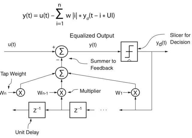
DFE is commonly implemented in high-speed links receiver side. DFE would subtract out

channel impulse responses from previous data bits to zero out ISI impacts on the current bit. If the

DFE has N taps, then the previous n-bits induced ISI can be mainly removed. The basic DFE

(24)

12

Figure 2.4. Basic DFE working mechanism

DFE can boost high frequency content without noise and crosstalk amplification. For

example, Figure 2.5 shows a single bit response. The blue line is the original signal after the

channel. Because the long tail would interfere upcoming signals, the signal after the main cursor

should drop down quickly. DFE tap will erase the long tail by dragging post cursors down to zero.

If we have 2 DFE taps in the receiver, we can erase 2 UIs tail. The distance a1 and a2, in Figure

2.5, directly influence the DFE tap1 and tap2 value. Typically, each DFE tap value has a very

strong relation with the post cursor information. Figure 2.6 [25] shows two typical DFE corrected

data eyes. On the left is for the case when the dominant post-cursor ISI is positive, while on the

right negative. The left chart implies the congregated equalization before DFE is not enough, or

under-equalized, while the right chart indicates the congregated equalization is excessive, or

(25)

13

Figure 2.5. DFE tap function

Slicer makes a symbol decision without amplifying noise. The results are fed back to the

slicer input through a FIR filter to cancel post-cursor ISI. The major challenge in DFE

implementation is the closing timing on the first tap feedback, which must be done in one-bit

period or unit interval (UI).

Figure 2.6. Typical eye diagrams after DFE

2.2. IBIS-AMI model introduction

To analyze and simulate the performance of the entire SerDes link, behaviors of the TX

and RX need to be accurately modeled. Impairments should be considered inside the model.

However, such information is typically proprietary to SerDes vendors and unavailable to the user

(26)

14 model is proposed. The IBIS-AMI model is a powerful method to incorporate SerDes and channel

models into a unified simulation environment which protects vendors’ intellectual property. The

IBIS-AMI model is a behavior model and shows a high correlation with the on-die circuit.

2.2.1. How does the IBIS-AMI model work

Input/output Buffer Information Specification (IBIS) models were first generated by Intel

in 1993. As the chip designs became more and more complex, traditional IBIS models could no

longer keep up with the DSP design. Vendors were again providing their own encrypted models

which were platform specific. Thus, the IBIS community worked to extend the IBIS models and

IBIS-AMI models were born. IBIS-AMI model represents an important milestone in the IBIS

mixed-signal evolution [31].

AMI stands for Algorithmic Modeling Interface. It is designed to handle modeling of the

algorithmic functions of an I/O. IBIS-AMI models provide the end user with the model portability

that they need while ensuring the vendors that their IP is protected.

Figure 2.7 shows the same system with block level descriptions [34]. The channel contains

many parts which may be individually modeled. This includes the connectors, Printed Circuit

Board (PCB) traces, vias, and package models. The composite channel includes all of these with

the addition of the analog IBIS buffer models. The IBIS-AMI model has two modes, namely

statistical and time-domain simulation [16] [32]. Channel simulators make the assumption that this

composite channel is linear time invariant (LTI) system. In both modes, the IBIS-AMI simulations

begin by characterizing the channel’s impulse response in the time domain. This is typically

accomplished by generating a Heaviside step function at the transmitter’s analog buffer and

converting the response at the receiver’s analog buffer by calculating the impulse response using

(27)

15 IBIS-AMI terminology, an IBIS-AMI simulation processes the effects of the models’ filtering

functions quite differently for time-domain or statistical methods.

Figure 2.7. IBIS-AMI simulation description

2.2.2. IBIS-AMI model Development Challenges

The main challenge for the IBIS-AMI model development is that it requires lots of

experienced experts and lots of trial and errors to develop a model [34]. High speed mixed signal

IC designers and architects are not programmers. They are better equipped at dealing with various

circuit design or algorithm developments. However, IBIS-AMI model development requires much

different skills, such as skill in C/C++ coding, skill with the IBIS-AMI standard, skill on parsing

IBIS files. Oftentimes, the circuit designers or architects become AMI model developers and are

tasked to pull together disjoint pieces of their IC designs from incomplete IC specifications, from

Spice simulations and from cryptic MATLAB/C++ code [30]. These disjoint pieces may lead to

incomplete AMI models.

Moreover, designing an IBIS-AMI model needs detailed information about the circuit

design and lots of trial & errors to improve model performance. Normally, it takes a long design

(28)

16

2.3. System identification modeling approach

System identification is used to build models for dynamic systems based on measured input

and output pairs. A system identification model is more like a map between a set of explanatory

variables and a set of predicted variables [1] [2].

Generally, system identification models can be divided into two types, linear system

identification modeling, and nonlinear system identification modeling.

2.3.1. Linear System Identification Model

If one system can be presented as the following form, this system is called linear system.

y(#) = G('()_{)u(#) + H('}()_)e(#) _(2.1)

Where G and H are transfer functions in the time delay operator, q-1_{. e(t) is the white noise}

signal, which is independent of model inputs and outputs. The delay operator is shown below:

'(._{/(#) = /(# − 1)} _(2.2)

Where d is how many sampling points delay between input and output. The system

identification model is to use current and previous inputs and errors to predict the current output.

The basic configuration of linear system identification is shown in Figure 2.8. There are

two main linear system identification structures, AutoRegressive eXternal input (ARX) model and

AutoRegressive Moving Average eXternal input (ARMAX) model.

Figure 2.8. Linear system identification configuration

In ARX model, the current output is related to the previous inputs and outputs. It doesn’t

consider white-noise disturbance. The ARX model can be obtained as

H

e (noise)

G

(29)

17

2(')3(#) = 4(')5(# − 6₇) (2.3)

where 2(') = 1 + 9)'()+ ⋯ + 9;<'(;< , 4(') = =) + =>'()+ ⋯ + =;?'(;?@).

In ARMAX model, the current output is related to the previous inputs, the previous outputs

and current and previous white-noise disturbance value. This means ARMAX model is more

general than the ARX model. The ARMAX model structure can be represented as

2(')3(#) = 4(')5(# − 6₇) + A(')B(#) (2.4)

where 2(') = 1 + 9₎'()_{+ ⋯ + 9}

;<'(;< , 4(') = =)+ =>'()+ ⋯ + =;?'(;?@) ,

A(') = 1 + C₎'()_{+ ⋯ + C}

;D'(;D.

2.3.2. Nonlinear system identification model

Nonlinear system identification model reuses the input structures from linear models and

changes the internal structure to a feedforward multilayer perceptron (MLP) network [3].

Nonlinear system identification model is more general than linear system identification models.

First, the internal structure is flexible to handle very complex nonlinear system. Second, it is easy

to handle by end users. Third, it is suitable for the design of control systems. The nonlinear system

identification formula is shown below:

3(#) = E[G(#, I)] + B(#) (2.5)

where φ(#, θ) is the regression vector and θ is the weights in the neural networks, and g is

(30)

18

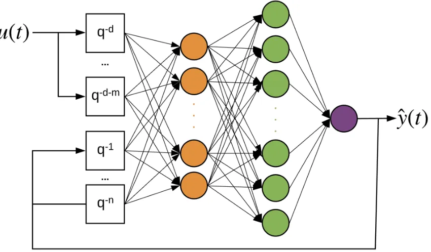
Figure 2.9. NNARX structure

The ARX model based on neural networks (NNARX) model structure is shown in Figure

2.9 [3]. The training process of the NNARX model is shown below:

1. The input and output orders are set; the weights and bias are initialed in the neural

networks.

2. After initialization, the model will do forward propagation and calculate the final output.

3. After that, it will calculate the loss function. In this work, mean square error (MSE) is

set as the loss function, which can be calculated as:

NOPP = 1

QR(3S − 3TS)>

U

SV)

(2.6)

where 3_S is the real output at sampling point i; 3T_S is the predicted value from the model

at sampling point i. Q is the total number of data points.

4. Next, the model will update the weights and bias in the neural networks by the

(31)

19

WY = WX X_{− [ ∗ 1W}X

=] = =X X_{− [ ∗ 1=}X

(2.7)

WX _and₌X _{are the current weights and bias at each layer}_^_._1WX_and₁₌X_{are partial}

derivatives of loss function. [ is the learning rate. WYX_and₌]X_{are updated weights and}

bias at each layer ^.

5. After updating the weights and bias, it will go back to step 2 and repeat until the loss

function is very small or the max number of learning step is reached.

This model structure is similar to the DFE structure in a receiver. The DFE has output

feedbacks, which would influence the current output value. Meantime, the NNARX also has output

feedbacks. The DFE has a slicer, which is a nonlinear component and used to quantize the inputs.

In NNARX model, each neuron has an activation function, which is also nonlinear.

2.4. Deep learning model

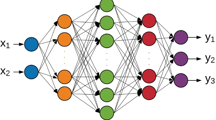
2.4.1. Deep neural networks model

Neural networks model is a technology to mimic the activity of the human brain [26]. It

can learn a black-box system. A simple application of the neural networks to do the data analysis

is called MLP. An MLP consists of at least three layers of nodes: an input layer, a hidden layer,

and an output layer. Except for the input nodes, each node is a neuron that uses a nonlinear

activation function, for example, sigmoid or tanh function. Each node in the hidden layer is a

function of the nodes in the previous layer. The output node is a function of the nodes in the hidden

layer. The number of neurons in the output layer depends on the number of outputs user set. MLP

uses backpropagation for the training process. Its multiple layers and non-linear activation

(32)

20 Compared with the MLP, deep neural networks (DNN) [27] increases the hierarchy of

complexity and abstraction. Figure 2.10 shows the DNN structure. Each layer applies a nonlinear

transformation onto its input and creates a statistical model as output from what it learned. The

input features are received by the input layer and passed into the first hidden layer. Each neuron

in the hidden layers has weights and biases. Each neuron has an activation function which is used

to standardize the output from the neuron. The “Deep” in deep neural networks means there is

more than one hidden layer in DNN. The output layer returns the output data. Until the output has

reached an acceptable level of accuracy, training epochs will be continued.

Figure 2.10. Deep Neural Networks structure

The number of neurons in each layer can be represented as {L} = (NS;_{, N})_{, … , N}c_{, N}def₎_,

where NS;_{, N}c_{, N}def_{are the number of neurons in the input layer,}_ℎfc_{hidden layer, and output}

layer respectively. The input of the ℎfc_{hidden layer can be calculated by}

{hc_{} = {/}c()_}Wc _(2.8)

where Wc_{is a matrix which contains the weights between the output of the}_{(ℎ − 1)}fc_layer

(33)

21

{/c_{} = i}

j({hc} + {=c}) (2.9)

where ij is the activation function. In this work, rectified linear unit (ReLU) [4] is used as

the activation function, which is obtained as

i_j(h) = max (0, h) (2.10)

The output from the output layer is the prediction targets, {3T}. In this research, three CTLE

adaptation results are the model prediction outputs. The weights, Wc_{, and bias,}₌c_{, of each layer}

are needed to be trained. The stochastic gradient descent (SGD) method [5] is used to minimize

the cost function, which can be represented as

Wc _{= W}c_{− γ∇]}

qr,srt ∀ℎ = 1, … 6, O5# (2.11)

where ∇]_qr_,srt is the stochastic approximation to the true gradient. γ is the learning rate

during the training process. The stochastic gradients are computed by the backpropagation method.

2.4.2. Long short-term memory (LSTM) model

As a state-of-the-art deep learning architecture is designed for time-series regression

problem. RNN is widely used in forecasting such problem [6]. The RNN aims to map the input

sequence x into outputs y. Each output in the sequence is calculated by the state of the previous

RNN cell and current input. To reduce the training complexity, the structures of each RNN cells

are the same. The unfolded topological graph is shown in Figure 2.11, which can demonstrate the

(34)

22

Figure 2.11. RNN unfolded topological graph

Traditional RNN or Vanilla RNN (VRNN) structure faces a challenge. If the training length

of RNN is significantly long and non-truncated backpropagation is applied, due to a vanishing

gradient or exploding gradient, backpropagated errors will get smaller or larger layer by layer,

which makes backpropagation insignificant. To deal with the vanishing gradient or exploding

gradient problems, the LSTM model is proposed [7]. The LSTM cell structure is shown in Figure

2.12. LSTM can create paths where the gradient can flow for a long duration.

Figure 2.12. LSTM cell structure

The core function of the LSTM is the cell state, which is the horizontal line on the top of

Figure 2.12. The cell state would go through the entire chain, with some linear interactions. The

LSTM has the capability to remove or add previous or new information to the cell state using gates.

(35)

23 networks layer and a pointwise multiplication operation. An LSTM cell has three gates, namely

input, output and forget, to protect and control the cell state. The input gate would add new

information selected from the current input and previous sharing parameter vector into the current

cell. The forget gate is to discard useless information from the current memory cell. And the output

gate decides new sharing parameter vector from the current memory cell.

At first, LSTM would discard useless information from the cell state. This decision is made

by a sigmoid layer named the forget gate layer. It looks at ht-1 and xt, and outputs a number between

zero and one for each number in the cell state Ct-1. If the output is one, it means the LSTM would

completely keep the cell state, while zero represents the LSTM would completely forget this. The

forget gate can be calculated as

i_f = v(W_w∙ [ℎ_f(), /_f] + =_w) (2.12)

where i_f is the output of the forget gate. W_w and =_w are the weights and biases of the neural

networks. ℎ_f() is the previous hidden vector. /_f is the current input.

The next step is to decide what new information is needed to store in the cell state. This

step is twofold. First, a sigmoid layer named the input gate layer, decides which values will be

updated. Next, a tanh layer creates a vector of new candidate values, C̃t, which could be added to

the state. Second, these two will be combined to create an update to the state. The input gate can

be represented by

y_f = v(W_S ∙ [ℎ_f(), /_f] + =_S)

Az_f = #96ℎ(W_{∙ [ℎ_f(), /_f] + =_{) (2.13)

where y_f is the output of the input gate layer. W_S and =_S are the weights and biases of the

input gate layer. Az_f are the vectors which modify the cell state.

(36)

24

Af = if∗ Af()+ yf∗ Azf (2.14)

where A_f is the new cell state. i_f and y_f are the outputs of the forget gate and input gate

respectively. These two gate outputs will decide how much information will be through away and

updated, which can be obtained as

i_f = v|W_w∙ [A_f(), ℎ_f(), /_f] + =_w}

y_f = v(W_S∙ [A_f(), ℎ_f(), /_f] + =_S)

O_f = v(W_d∙ [A_f, ℎ_f(), /_f] + =_d)

(2.15)

Finally, the LSTM cell will decide what should be considered as the final output. A sigmoid

layer will decide what parts of the cell state are the output. Then, the cell state, Af, will go through

a tanh layer and multiply it by the output of the sigmoid gate. The output of the LSTM can be

obtained by

Of = v(Wd∙ [ℎf(), /f] + =d)

ℎ_f = O_f∗ tanh (A_f) (2.16)

where O_f is the output of the output gate. ℎ_f is the final output of the LSTM. W_d and =_d are

the weights and biases of the output gate layer.

With these three gates, the LSTM model will remember all the useful information from the

(37)

25

Chapter 3. State-of-the-Art

Recently, numerous works have been done in high-speed receiver behavioral modeling to

speedup post-silicon validation [8]. In this chapter, we would present the state-of-the-art receiver

behavioral modeling using machine learning approach. The high-speed receiver behavioral

modeling can be divided into two areas: 1) receiver transient behavior modeling and 2) receiver

adaptation modeling.

3.1. Receiver transient behavioral modeling

The receiver transient behavior modeling has two modeling methods: grey-box modeling

method and black-box modeling method. The grey-box modeling methods are used to predict only

eye height and eye width. The black-box modeling methods would predict the receiver transient

output waveforms.

As for the eye margin prediction problem, in [9], a grey-box modeling method is presented.

They took a deep look into their circuit, extracted 10K features and selected 30 features, using

feature selection method, to predict eye height and eye width at the receiver. They did a

classification and regression prediction of eye margin. As for eye margin classification prediction,

they set a threshold and used couples of machine learning models, like Random Forest, Boosted

Trees, to predict whether the eye is passed or failed. As for eye margin prediction, they used

machine learning regression models, like Random Forest, SVM, to predict eye height and eye

width respectively. The results showed that all the model prediction accuracies are low. The

worst-case testing accuracy is only 87%. Because it’s a grey-box modeling method, they need some

SerDes experts to handle parameters in the receiver and examine whether the selected features are

reasonable. [10] used Artificial Neural Networks (ANN) to predict eye width and eye height after

(38)

26 number of knobs. They tested their methodology on two current industrial high-speed channel

topologies, namely USB3 SuperSpeed Gen1 and SATA Gen 3. It’s a grey-box modeling method

because they need to use domain knowledge to select 7 and 10 important receiver knobs for USB3

SuperSpeed Gen1 and SATA Gen 3 respectively. Using a system response sampling strategy, their

model accuracies are around 95% for eye width and eye height prediction. However, their receiver

model doesn’t include DFE, which is a non-linear component in the receiver. The DFE is

commonly used in most of the high-speed SerDes systems. Meanwhile, it’s not practical to only

predict eye width and eye height in the SerDes system. [12] uses the DNN model to predict eye

width and eye height using 8 human-selected features in the SerDes channel. Again, their receiver

model doesn’t include the DFE block, and their model can only predict eye width and eye height.

[28] and [29] presented SVM models to predict the eye height and eye width using five selected

features. The prediction results didn’t show a very high correlation.

The eye width and eye height measurement only contain four data points in an eye diagram,

which cannot be used to plot bathtub curves. The bathtub curve shows the horizontal or vertical

eye-opening at each bit error rate (BER) level. It is based on the jitter probability density function,

which can be only extracted from an eye diagram.

In a SerDes system, there are approximately thousands of circuit features impacting the

recovered signal in SerDes receiver. The published grey-box methods take a couple out of the

thousands of features to build the ML model and do prediction. The tradeoff in the grey-box

modeling method is the more features adopted in the ML model the more accurate the prediction

but the model complexity and simulation time increase. The accuracy of the grey-box method will

(39)

27 As for the transient waveform prediction, [14] uses a system identification modeling

method to predict the receiver output waveforms. However, they didn’t validate their model using

eye diagrams and only a few bits are tested. [11] and [12] presented a black-box modeling method

to predict transient waveforms at the receiver, which can be used to plot eye diagrams. Deep

learning models namely stacked Recurrent Neural Networks (RNN) and stacked Long Short-Term

Memory (LSTM) model, are trained based on PRBS data. However, the current black box training

methods can only predict the transient waveforms from the same PRBS data set and the same

channel that the training data are from. But they did not provide any information about waveform

prediction accuracy. And they need continuous training transient waveforms to feed into their

model to obtain high accuracy. Meanwhile, either the RNN or LSTM model has very long training

time, normally several hours or even a day, with a very-long-bit PRBS data sequence. What’s more,

due to their model accuracy limitation, the eye diagram generated from predicted transient

waveform shows a low correlation with the real eye. Also, their test data are less than 100 UIs,

which are not enough to test their model accuracy. As for signal integrity analysis, they only did

the eye diagram comparison.

According to the recent works, there are no modeling methods which can only train the

machine learning model once and predict the transient waveforms, not from the same training

PRBS data and training channel. Moreover, some publications provide prediction accuracy while

some do not. The provided accuracy numbers are all about eye height and eye width prediction

without giving the accuracy number for predicted transient waveforms.

Nowadays, no publications are found to do bathtubs prediction. The bathtub prediction is

based on the eye diagram constructed from long enough transient waveforms. Generally, it needs

(40)

28 time and consequently, the total length of the transient waveform prediction can be obtained with

reasonable simulation time. All the latest published work can predict much fewer bits required for

bathtub prediction.

The proposed modeling method in this work provides fast and high-precision simulation

results for the transient waveform, eye diagram and bathtub curve.

3.2 Receiver adaptation modeling

With the transceiver becoming more and more complex, it’s impossible to tune these

parameters manually. In that case, equalization adaptation techniques for the on-die circuit are

proposed [36] [37] [38] [39] [40]. An adaptive tuning approach allows the optimization of the

equalizers for varying channels, environmental conditions, and data rates. One of the commonly

used CTLE adaptation technique is CTLE tuning with output amplitude measurement [37]. As for

the DFE adaptation, [39] proposed 2x oversampling the equalized signal at the edges can be used

to extract information to adapt a DFE and drive a CDR loop, and sign-sign least mean square (LMS)

algorithm used to adapt DFE tap values.

Nowadays, only IBIS-AMI model has the capability to provide the adaptation simulation

[15]. To find the best receiver coefficients, LMS adaptation methods are used. The LMS algorithm

is an approximate gradient descent optimizer [53]. Its objective function is the mean squared error

between the equalizer output and the desired equalizer output, which is assumed to be the

transmitted waveform 1(#), sampled at the center of the eye pattern. Letting B(ÅÇ) = 1(ÅÇ) −

É(ÅÇ), the mean square error is

(41)

29 The approximation comes in using the instantaneous value of the squared error as a noisy

estimate of its expected value. A constant Ö is defined to control the adaptation’s rate of

convergence. The result is the familiar LMS update equation

Ü⃗(ÅÇ) = Ü⃗(ÅÇ − Ç) + 2ÖB(ÅÇ)Ö⃗(ÅÇ) (3.2)

Hence, the LMS algorithm would minimize the mean squared error and find the best

receiver settings.

However, the IBIS-AMI model has some limitations. The IBIS-AMI model can only do

adaptation and transient simulation at the same time, which would be inefficient in two scenarios.

The first scenario is that users want to get transient simulation results to see the eye-opening or

bathtub curve information. The second scenario is that users only need to know the receiver

adaptation codes, which represent the equalization status of the SerDes link. In that case, we need

to find a way to build behavioral models for these two simulations separately, while the simulation

speed of the behavioral models should be faster than the IBIS-AMI model.

To the best of our knowledge, there is no work focusing on the SerDes receiver adaptation

behavioral modeling using the machine learning approach. The reason why no one touches this

area is that the response of the system is dynamic. In the LTI system, the response of the system

is linear and won’t change during the observation. The adaptation process in the high-speed SerDes

link is a non-LTI system, which is difficult to build a behavioral model.

In this work, the proposed modeling mechanism can show a high correlation with the

receiver adaptation codes in the on-die circuit. Meanwhile, the simulation speed of the proposed

(42)

30

Chapter 4. Receiver transient behavioral modeling

It’s crucial to build the SerDes behavioral models with high simulation speed and good

hardware correlation. The current SerDes simulation model, IBIS-AMI model, takes thirty minutes

to do the transient simulation. In this chapter, we focus on building a high-speed SerDes receiver

equalized transient behavior model, which has a fast simulation speed and excellent correlation.

At first, we explored various machine learning model types using the data collected from

a 10 Gbps Avago transceiver and select the best model type for the transient modeling. Second, a

different transceiver, Xilinx UltraScale+ GTY transceiver, is used to collect data and test the

robustness of the selected model type. Xilinx UltraScale+ GTY transceiver is a 100 GE application,

which the data rate is 25Gbps. To further improve model performance, an adaptive-ordered system

identification model is proposed to mimic the behavior of the high-speed receiver. Transient

waveform, eye diagram and bathtub curve are used as the model performance metrics.

4.1. Model type exploration

At the beginning of this research, a 10 Gbps Avago transceiver is used to collect data. Next,

how to collect the data and do the model training are briefly introduced.

4.1.1. Data collection

Figure 4.1 shows how to measure the receiver input and output using the scope. To collect

various cases, different data pattern, TX settings, backplane channels, and RX settings are swept.

(43)

31

Figure 4.1. Data measurement from the 10 Gbps Avago transceiver

Table 4.1. Avago transceiver setting configuration

configurations

Data rate 10 Gpbs

Data Pattern PRBS7

Channel insertion loss Low, medium, high

TX settings Low, medium, high swing

RX CTLE Gain Low, medium, high

DFE Off, on

During the data collection, the receiver equalization setting is fixed, and the system

response is stable. Our goal is to build a receiver behavioral model under a fixed receiver setting.

In this experiment, because there are 3 different channels for the Avago chip, CTLE and

DFE settings are tuned to make eye open reasonably large for different channels. CTLE settings

include DC gain, low-frequency gain and high-frequency gain. As for the DFE, the first two DFE

tap values are considered and other DFE taps are set as zero gain. In this experiment, 3 CTLE and

2 DFE settings are tuned under three different channels. The criterion is to make sure it would pass

the eye mask test at the receiver for each measured case, which ensures that the signal-to-noise

(44)

32 behavior but not random noise. If the signal-to-noise ratio is small, the model predicted accuracy

would drop because of the random noise. In this experiment, the receiver input and output

waveforms for 50 different CTLE and DFE settings cases are measured. Those 50 receiver settings

are from three different channels. Both receiver input waveform and output waveform are

measured using the real-time oscilloscope. The receiver input and output waveform would be the

input and output of the model. The number of measured input bits and output bits are 7128. The

data rate is 10Gbps. As for the data measurement, there are 16 sampling points per UI.

4.1.2. Model performance comparison

There are 5 different model types considered in this work. Recall in Section 2.2, system

identification models can be divided into two types, linear system identification modeling, and

nonlinear system identification modeling. In the linear system identification modeling, ARX and

ARMAX model are considered in this work. As for the nonlinear system identification modeling,

NNARX model is used. RNN model, which is often used in time-series data prediction problem,

is also used in this research.

As for the model accuracy validation, we use the normalized root mean square accuracy

(NRMSA). This method is commonly used in time series data prediction problem. The NRMSA

can be calculated as

âäãå2 = 100 × é1 − è∑ëSV)(3S− 3TS)>

∑ë (3_S − 3í)>

SV)

ì _(4.1)

where yi is the real output at time i. 3T_S is the model predicted output at time i, and 3í is the

mean of all the real outputs. If the predicted output is close to the real data, the NRMSA is close

(45)

33 As for the system identification models, the input and output orders mean how many

previous inputs and outputs should be considered to predict the current output. To simplify the

model process, we set the input order equal to the output order in the system identification model.

If only a few past inputs and outputs are considered, which means the orders of input and output

are low, the model accuracy would be low. On the other hand, if too many past inputs and outputs

are chosen, which means the orders of input and output are high, the model would be more complex

and training time increases. Choosing the best trade-off point is the key to building model process.

Order sweeping method is used for selecting the best order of each model.

In this experiment, the order sweeping method is used to select the best orders of the ARX,

ARMAX, and NNARX model. What’s more, to reduce the sweeping iteration, the order of inputs

and outputs of the models are set as the same.

In this work, for nonlinear system identification models, twenty hidden neurons with tanh

activation function in one hidden layer and one linear output neuron are set in neural networks

architecture. For the LSTM model, the batch size is set to 100. 200 hidden units are used in each

LSTM cells. The learning rate is 0.004.

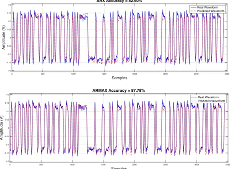
Figure 4.2 shows prediction results of one case for linear system identification models,

nonlinear system identification models, and LSTM model respectively. This is the case that only

CTLE works.

As for linear system identification models, ARX model shows low correlation with the real

data. ARX model cannot predict the low and high frequency gain accurately. On the other hand,

the performance of the ARMAX model is a little better than ARX model. It can predict the high

frequency gain accurately, but not the low frequency gain. The worst accuracies for the ARX and

(46)

34

Figure 4.2. Linear system identification model performance

As for nonlinear system identification model, shown in Figure 4.3, the NNARX model

shows high correlations with the real data. Both models can predict the low and high frequency

gain accurately. The worst accuracies for the NNARX model is 93.11%.

As for the LSTM model prediction in Figure 4.4, it also shows a high correlation with the

real waveform. The LSTM model can predict the low and high frequency gain accurately. The

worst accuracy for the LSTM model is 93.07%. However, the prediction accuracy of the LSTM

model is lower than the nonlinear system identification models. What’s more, the training time of

the LSTM model is much longer than system identification models.

0 500 1000 1500 2000 2500 3000 3500

Samples -0.2 -0.15 -0.1 -0.05 0 0.05 0.1 0.15 0.2 Amptitude (V)

ARX Accuracy = 82.60%

Real Waveform Predicted Waveform

0 500 1000 1500 2000 2500 3000 3500

Samples -0.2 -0.15 -0.1 -0.05 0 0.05 0.1 0.15 0.2 Amptitude (V)

ARMAX Accuracy = 87.78%

(47)

35

Figure 4.3. Nonlinear system identification model performance

Figure 4.4. LSTM model performance

The model performances for all the 50 cases are shown in Figure 4.5. For linear system

identification models, the ARMAX model shows better performance than ARX model. The orders

the ARX and ARMAX models are 20, which means previous 20 sampling points of input and

output data are used to predict the current output. The orders the NNARX models are 10. Nonlinear

system identification model and the LSTM model have similar model performance. However, the

average prediction accuracies of the LSTM model and NNARX model are 95.71% and 95.78%

respectively. What’s more, the average worst case accuracies of the LSTM model and NNARX

model are 93.23% and 92.96% respectively. The performance of the NNARX model is better than

the LSTM model.

0 500 1000 1500 2000 2500 3000 3500

Samples -0.2 -0.15 -0.1 -0.05 0 0.05 0.1 0.15 0.2 Amplitude (V)

NNARX Accuracy = 96.02%

Real Waveform Predicted Waveform

0 500 1000 1500 2000 2500 3000 3500

Samples -0.2 -0.15 -0.1 -0.05 0 0.05 0.1 0.15 0.2 Amplitude (V)

LSTM Accuracy = 95.26%

(48)

36

Figure 4.5. Model performances for 50 cases

As for the transient simulation, the simulation speed of the model is also important. The

IBIS-AMI model takes 30 minutes to simulate half million bits. For the linear and nonlinear system

identification models, due to its simple model structure, all the models need around 10 seconds for

half million-bit simulation. However, it takes about 5 minutes for the LSTM model simulation.

Here are the reasons why the NNARX model’s performance is better than the LSTM model:

1) To overcome vanishing gradient problem, the LSTM model have three gates, which

can bypass units and remember for longer time steps [18]. Since the LSTM model can

remember information happened very long time ago, too much unrelated information

is considered to predict the current output. The advantage of the LSTM model is

suitable in the sequence prediction but not in the receiver behavioral modeling because

the current output is only influenced by the recent previous bit due to the channel loss.

2) When the DFE is involved, the current output depends on previous bit values. How

many DFE taps the receiver has decides how many previous bit values are going to

effect on the current bit value. The LSTM model can remember previous information

70 75 80 85 90 95 100

1 2 3 4 5 6 7 8 9 10 11 12 13 14 15 16 17 18 19 20 21 22 23 24 25 26 27 28 29 30 31 32 33 34 35 36 37 38 39 40 41 42 43 44 45 46 47 48 49 50

TD

ac

cu

rac

y

(%

)

Test cases

Model Time Domain Accuracy for 50 Cases

(49)

37 long time ago, which doesn’t match the DFE feedback structure. On the other hand, the

memory depth of the nonlinear system identification is the order of the input and the

output, which set by users (adaptive-ordered system identification model will be

introduced in the next Section). In that case, only a few recent information would be

used, in the nonlinear system identification model, to predict the current output, which

increases the correlation among the model inputs and outputs.

3) The LSTM model as a complex the model structure, which makes the training time

become slower than other models. On the contrary, the nonlinear system identification

model has a simpler structure.

Considering the model performance and simulation speed, the NNARX model is the best

model type for the receiver equalized transient behavioral modeling.

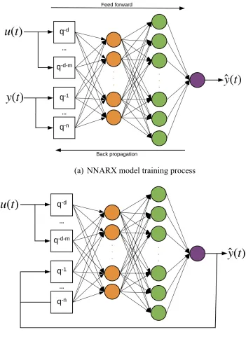
4.1.3. NNARX model training and prediction process

The NNARX model is a recurrent dynamic network, with feedback connections enclosing

several layers of the network. The NARX model is based on the linear ARX model, which is

commonly used in time-series modeling.

The defining equation for the NARX model is:

3(#) = i(3(# − 1), … , 3|# − 6î}, 5(# − 1), … , 5(# − 6e)) (4.2)

where the next value of the dependent output signal y(t) is regressed on previous values of

the output signal and previous values of an independent (exogenous) input signal. In the NNARX

model, function i is a feedforward neural network. A diagram of the NNARX model training

process is shown in Figure 4.6 (a). Since the true output is available during training, the true output

itself can be used instead of feeding back the estimated output. This will have two advantages. The

(50)

38 the static back propagation can be used for training instead of dynamic back propagation, which

has complex error surfaces exposing the network to higher chances of getting trapped in local

minima and hence requiring a greater number of training iterations.

Once the outputs have been calculated, the NNARX model would compute the error E,

which is defined by the expression:

t =1

2R(3S − 3ñ)ï >

ë

SV)

(4.3)

where 3ñï is the model predicted output and 3S is the desired output. The most commonly

used learning algorithm is the gradient descent algorithm. In this the global error calculated is

propagated backward to the input layer through weight connections as in Figure 4.6 (a). During

the back-propagation process, Levenberg-Marquardt algorithm [51] is used in the model, which

can be written as

W_;óò= W_dX. − [ôö_{+ õú]}()_ôö_t(W

dX.) (4.4)

Where ô is the Jacobian matrix that contains first derivatives of the network errors with

respect to the weights and biases, ú is the identity matrix and õ is the parameter used to define the

iteration step value. It minimizes the error function while trying to keep the step between old

weights (W_dX.) and new updated weights (W_;óò).

After the NNARX model is well-trained, the prediction process of the NNARX model is

shown in Figure 4.6 (b). The next value of the dependent output signal y(t) is regressed on previous

values of an independent (exogenous) input signal. The output of NNARX network can be

considered to be an estimate of the output of some non-linear dynamic system that is being

(51)

39 architecture. In this way, the NNARX model can predict the current output based on previous

inputs and predicted outputs.

(a) NNARX model training process

(b) NNARX model prediction process

High-speed Receiver Behavioral Modeling Using Machine Learning.

DEDICATION

BIOGRAPHY

ACKNOWLEDGMENTS

TABLE OF CONTENTS

LIST OF TABLES

LIST OF FIGURES

Chapter 1.

Introduction

1.1. Motivation

1.2. Contribution

1.3. Organization

1.4. Abbreviations

Chapter 2.

Background and Fundamentals

2.1. SerDes Background

2.1.1. Basics of CTLE

2.1.2. Basics of DFE

2.2. IBIS-AMI model introduction

2.2.1. How does the IBIS-AMI model work

2.2.2. IBIS-AMI model Development Challenges

2.3. System identification modeling approach

2.3.1. Linear System Identification Model

H

e (noise)

G

2.3.2. Nonlinear system identification model

2.4. Deep learning model

2.4.1. Deep neural networks model

2.4.2. Long short-term memory (LSTM) model

Chapter 3.

State-of-the-Art

3.1. Receiver transient behavioral modeling

3.2 Receiver adaptation modeling

Chapter 4.

Receiver transient behavioral modeling

4.1. Model type exploration

4.1.1. Data collection

4.1.2. Model performance comparison

4.1.3. NNARX model training and prediction process